Volume 33 - Article 32 | Pages 939–950

(1)

DEMOGRAPHIC RESEARCH

VOLUME 33, ARTICLE 32, PAGES 939–950

PUBLISHED 3 NOVEMBER 2015

http://www.demographic-research.org/Volumes/Vol33/32/ DOI: 10.4054/DemRes.2015.33.32

Descriptive Finding

Residential mobility in early childhood:

Household and neighborhood characteristics of

movers and non-movers

Elizabeth Lawrence

Elisabeth Dowling Root

Stefanie Mollborn

This open-access work is published under the terms of the Creative Commons Attribution NonCommercial License 2.0 Germany, which permits use, reproduction & distribution in any medium for non-commercial purposes, provided the original author(s) and source are given credit.

(2)

1 Introduction 940

2 Methods 941

3 Results 942

4 Discussion 946

5 Acknowledgements 947

(3)

Demographic Research: Volume 33, Article 32

Descriptive Finding

Residential mobility in early childhood: Household and

neighborhood characteristics of movers and non-movers

Elizabeth Lawrence1 Elisabeth Dowling Root2

Stefanie Mollborn3

Abstract

BACKGROUND

Understanding residential mobility in early childhood is important for contextualizing influences on child health and well-being.

OBJECTIVE

This study describes individual, household, and neighborhood characteristics associated with residential mobility for children aged 0−5.

METHODS

We examined longitudinal data from the Early Childhood Longitudinal Study-Birth Cohort (ECLS-B), a nationally representative sample of children born in 2001. Frequencies described the prevalence of characteristics for four waves of data and adjusted Wald tests compared means.

RESULTS

Moving was common for these families with young children, as nearly three-quarters of children moved at least once. Movers transitioned to neighborhoods with residents of higher socioeconomic status but experienced no improved household socioeconomic position relative to non-movers.

CONCLUSION

Both the high prevalence and unique implications of early childhood residential mobility suggest the need for further research.

1_{Carolina Population Center, University of North Carolina, Chapel Hill. E-Mail: [email protected].} 2_{College of Public Health and Department of Geography, The Ohio State University.}

(4)

1. Introduction

Research shows that residential mobility shapes child well-being. Children who stay in the same home have better behavioral and emotional health and educational achievement than their more mobile counterparts (Jelleyman and Spencer 2008; Leventhal and Newman 2010; Ziol-Guest and McKenna 2014). The mechanisms behind these associations include changes in social relationships such as friendship networks (South and Haynie 2004) and disruptions in institutional supports such as health insurance or medical facilities (Busacker and Kasehagen 2012). Complicating causal interpretation of observed associations are the many confounding factors that influence both mobility and well-being. For example, Dong and colleagues (2005) reported that adverse childhood experiences, such as childhood abuse, are associated with residential mobility and explain the effect of frequent moving on health risks. Controlling for selection is therefore important for determining the effects of residential mobility, since mobile and non-mobile families differ in many ways (Gasper, DeLuca, and Estacion 2010). This is particularly important because some studies find that mobility exerts an independent influence on child well-being (Pribesh and Downey 1999) that cannot be examined without properly controlling for selection bias.

Further, moving does not necessarily have negative consequences, as many families move for positive reasons, such as a new or better job or to have a child attend a chosen school. Prior research has found differential effects of mobility depending on neighborhood context, child’s age/developmental period, and financial resources (Anderson, Leventhal, and Dupere 2014; Pettit 2004). Giving birth to a young child may precipitate a particular type of move, since this life course change can spur relocation efforts (Mulder and Hooimeijer 1999; Rabe and Taylor 2010). It is therefore important to examine mobility among young children separately from other groups.

Researchers usually operationalize mobility based on a short window of time prior to the interview, excluding the influence of moves earlier in life. Yet early development shapes later development (Willson, Shuey, and Elder 2007). Further, social influences show a cumulative process over time. Evidence points to the importance of childhood circumstances for adult health outcomes (Gruenewald et al. 2012; Haas 2008; Hayward and Gorman 2004). Examining mobility at the youngest ages is therefore crucial for understanding both the effects of mobility on child health and well-being and how residential mobility is influenced by a variety of individual, family, and neighborhood constraints.

(5)

longitudinal nationally representative data that describes families with children ages 0-5. We describe levels of mobility (defined by number of moves) across ages 0-5 and the family and neighborhood characteristics that are associated with these different levels. To our knowledge, this study is the first to examine early childhood residential mobility over time using a nationally representative sample. By describing mobility patterns across dynamic household and neighborhood characteristics, we provide context for future studies that seek to examine the effects of child residential mobility and health.

2. Methods

We used all waves of data from the Early Childhood Longitudinal Study-Birth Cohort (ECLS-B), which followed a nationally representative cohort of U.S. children born in 2001 at approximately 9 months, 2 years, 4 years, 5 years, and 6 years of age. Since the last wave of data only included a subsample of children who had not yet started kindergarten in the fourth wave, household and neighborhood information at kindergarten start (termed Wave K) was taken from either the fourth or fifth wave.. The ECLS-B dataset is uniquely suited for this study because it covers early childhood and its longitudinal design does not exclude movers (Snow et al. 2009).

Approximately 6,350 children had a valid kindergarten sampling weight and the biological mother as the respondent for all waves. Of these, 6,250 had complete data on moving. Some parents reported that they did not move, but the data showed they changed ZIP codes. Because we do not know the source of the error, we dropped these children (N≈150). The resulting sample size is 6,100 (96%). Some indicators had missing data, resulting in a sample reduction ranging from 0%−3% for each measure. All numbers reported here were rounded to the nearest 50 per NCES security requirements. Adjusted Wald tests compared means across mover statuses. We adjusted for complex sample design using jackknife replication weights.

(6)

Individual and household socio-demographic measures were derived from constructed ECLS-B variables and parent interviews. Individual measures included sex, race, and age (in months) of the child at each wave. We also included the following household indicators at each wave: mother’s educational attainment (in years), mother’s marital status, and income-to-needs ratio (the ratio of the household income to the year and household size-specific poverty threshold). Mother’s age at birth of the focal child and her first child were also examined.

For residential location measures, we used region (Northeast, Midwest, South, and West), urbanicity (urbanized area [population > 50,000], urbanized cluster [population > 2500 and <50,000], or rural [population<2500]), ZIP code characteristics, and parent-reported neighborhood safety. ZIP code of residence was used as a proxy for neighborhood (a limitation of the ECLS-B dataset, as this was the only geographic identifier collected), and characteristics were extracted from the 2000 Census SF3. ZIP code characteristics included the percentage of the population living below poverty, the percentage with a college degree, the median household income, and the percentages White, Black, and Hispanic. Townsend and Carstairs indices were also developed from census data and capture material deprivation in the neighborhood (Carstairs and Morris 1991; Townsend, Phillimore, and Beattie 1988). ECLS-B offered one survey item of parent perceptions of the neighborhood that is consistent across waves. Parents were asked to report whether they believed their neighborhood is safe from crime, and responses were dichotomized into those reporting very safe and those reporting fairly safe, fairly unsafe, and very unsafe. All parents answered this question in Wave 2, but only parents who reported having moved since the last wave were asked this question in Waves 3 and K.

3. Results

(7)

to 4.0 in Wave K and those moving three or more times increased from 1.9 to 2.2. Even though the levels of income-to-needs differed at each of the waves, the change over time did not significantly differ, signifying that both groups made gains at about the same rate.

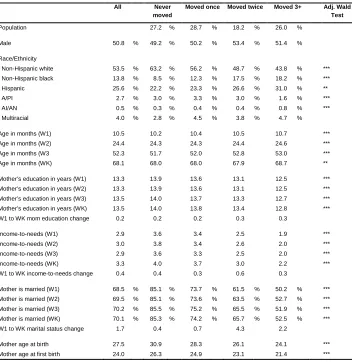
Table 1: Individual and household characteristics, across mover categories

All Never

moved

Moved once Moved twice Moved 3+ Adj. Wald Test

Population 27.2 % 28.7 % 18.2 % 26.0 %

Male 50.8 % 49.2 % 50.2 % 53.4 % 51.4 %

Race/Ethnicity

Non-Hispanic white 53.5 % 63.2 % 56.2 % 48.7 % 43.8 % *** Non-Hispanic black 13.8 % 8.5 % 12.3 % 17.5 % 18.2 % *** Hispanic 25.6 % 22.2 % 23.3 % 26.6 % 31.0 % ** A/PI 2.7 % 3.0 % 3.3 % 3.0 % 1.6 % *** AI/AN 0.5 % 0.3 % 0.4 % 0.4 % 0.8 % *** Multiracial 4.0 % 2.8 % 4.5 % 3.8 % 4.7 %

Age in months (W1) 10.5 10.2 10.4 10.5 10.7 *** Age in months (W2) 24.4 24.3 24.3 24.4 24.6 *** Age in months (W3 52.3 51.7 52.0 52.8 53.0 *** Age in months (WK) 68.1 68.0 68.0 67.9 68.7 **

Mother’s education in years (W1) 13.3 13.9 13.6 13.1 12.5 *** Mother’s education in years (W2) 13.3 13.9 13.6 13.1 12.5 *** Mother’s education in years (W3) 13.5 14.0 13.7 13.3 12.7 *** Mother’s education in years (WK) 13.5 14.0 13.8 13.4 12.8 *** W1 to WK mom education change 0.2 0.2 0.2 0.3 0.3

Income-to-needs (W1) 2.9 3.6 3.4 2.5 1.9 *** Income-to-needs (W2) 3.0 3.8 3.4 2.6 2.0 *** Income-to-needs (W3) 2.9 3.6 3.3 2.5 2.0 *** Income-to-needs (WK) 3.3 4.0 3.7 3.0 2.2 *** W1 to WK income-to-needs change 0.4 0.4 0.3 0.6 0.3

Mother is married (W1) 68.5 % 85.1 % 73.7 % 61.5 % 50.2 % *** Mother is married (W2) 69.5 % 85.1 % 73.6 % 63.5 % 52.7 % *** Mother is married (W3) 70.2 % 85.5 % 75.2 % 65.5 % 51.9 % *** Mother is married (WK) 70.1 % 85.3 % 74.2 % 65.7 % 52.5 % *** W1 to WK marital status change 1.7 0.4 0.7 4.3 2.2

Mother age at birth 27.5 30.9 28.3 26.1 24.1 *** Mother age at first birth 24.0 26.3 24.9 23.1 21.4 ***

Source: ECLS-B (2001-2007).

(8)

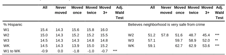
Table 2 displays neighborhood and geographic characteristics over time. In contrast to household factors, neighborhood characteristics generally improved among movers relative to non-movers. The Townsend Index, a measure of relative deprivation, shows a distinct downward trend among all movers (lower scores indicate less deprivation). Although there was a stark contrast in this measure at Wave 1 for non-movers compared to non-movers, there was no significant difference at Wave K across mover status, and the change in the Townsend Index from Wave 1 to Wave K differed significantly across mover status. Figure 1, Panel A visually presents the convergence over time for the Townsend index. Similar trends were observed for the other ZIP code characteristics, with differing magnitudes. Figure 1, Panel B illustrates the improvements in percentage of residents in poverty for movers, with those moving only once displaying similar values at Wave K to non-movers.

Figure 1: Means of neighborhood characteristics over time, by mover status

A Townsend Index B Percentage of households below poverty

C Percentage of residents that are non-Hispanic D Believes neighborhood is very safe from crime

Non-movers Moved once Moved twice X X X Moved 3+ times

Source: ECLS-B (2001-2007).

Notes: Adjusted for complex sampling design. N≈6100. * p<.05 ** p<.01 *** p<.001

1.0 1.2 1.4 1.6 1.8 2.0 2.2

W1 W2 W3 WK

*** ** ns ns

10.0 11.0 12.0 13.0 14.0 15.0

W1 W2 W3 WK

*** *** *** *** 60.0 62.0 64.0 66.0 68.0 70.0 72.0

W1 W2 W3 WK

*** *** ** * 40.0 45.0 50.0 55.0 60.0 65.0

W2 W3 WK

(9)

Table 2: Residential location characteristics, across mover categories

All Never moved Moved once Moved twice Moved 3+ Adj. Wald Test

Townsend Index Northeast

W1 1.7 1.3 1.8 1.9 2.0 *** W1 17.4 21.5 18.5 16.3 12.5 W2 1.6 1.3 1.6 1.8 1.8 ** W2 17.3 21.5 18.3 16.4 12.4 * W3 1.4 1.3 1.4 1.4 1.6 W3 16.9 21.5 18.0 15.5 12.0 * WK 1.3 1.3 1.3 1.3 1.4 WK 16.8 21.5 18.1 15.0 11.6 * W1 to WK change -0.4 0.0 -0.5 -0.5 -0.5 *** W1 to WK -0.6 0.0 -0.4 -1.4 -0.9 *

Carstairs Index Midwest

W1 0.7 0.4 0.6 0.9 1.1 *** W1 22.1 24.5 20.2 21.1 22.5 W2 0.7 0.4 0.6 1.0 1.0 *** W2 22.0 24.5 20.4 21.0 21.9 W3 0.5 0.4 0.4 0.6 0.8 *** W3 21.7 24.5 20.0 20.9 21.1 WK 0.5 0.4 0.3 0.6 0.8 ** WK 21.7 24.5 20.6 20.3 20.9 W1 to WK change -0.3 0.0 -0.4 -0.3 -0.4 *** W1 to WK -0.5 0.0 0.4 -0.9 -1.6 *

Living below poverty South

W1 13.0 11.5 12.7 13.7 14.5 *** W1 36.1 31.5 36.3 38.0 39.2 * W2 12.9 11.5 12.4 13.9 14.4 *** W2 36.3 31.5 36.4 38.6 39.6 * W3 12.5 11.5 11.9 13.0 14.0 *** W3 37.2 31.5 37.4 39.6 41.4 ** WK 12.3 11.5 11.6 12.9 13.6 *** WK 37.3 31.5 36.8 40.7 41.7 ** W1 to WK change -0.8 0.0 -1.2 -0.9 -1.0 *** W1 to WK 1.3 0.0 0.5 2.7 2.5 **

Median Household Income (in thousands) West

W1 44.5 47.7 46.2 43.1 40.3 *** W1 24.4 22.5 25.0 24.5 25.8 W2 44.7 47.7 46.6 42.8 40.6 *** W2 24.4 22.5 24.9 24.0 26.1 W3 45.5 47.7 47.1 44.6 41.7 *** W3 24.2 22.5 24.6 24.0 25.5 WK 45.7 47.7 47.6 44.7 42.1 *** WK 24.2 22.5 24.5 24.0 25.9 W1 to WK change 1.3 0.0 1.8 1.8 1.9 *** W1 to WK -0.2 0.0 -0.4 -0.5 0.0

% with College Education Urban

W1 23.5 25.0 25.2 22.6 20.7 *** W1 74.8 73.2 78.0 75.0 72.7 * W2 23.4 25.0 25.0 22.1 21.0 *** W2 74.2 73.0 77.4 73.8 72.0 * W3 23.4 25.0 24.7 22.2 21.1 *** W3 72.5 73.0 74.9 71.0 70.2 WK 23.5 25.0 25.0 22.5 20.8 *** WK 71.9 73.0 74.9 70.7 68.1 W1 to WK change 0.2 0.0 0.2 0.0 0.4 W1 to WK -2.8 -0.3 -3.1 -4.0 -4.1 **

% White Urban cluster

W1 65.5 69.6 65.1 63.2 63.2 *** W1 10.9 10.5 8.9 11.5 14.0 ** W2 66.1 69.6 66.0 64.0 63.9 ** W2 11.5 10.5 8.9 11.1 13.2 ** W3 67.1 69.6 67.9 64.9 65.2 ** W3 11.6 10.6 9.9 11.7 14.0 WK 67.5 69.6 68.4 65.1 66.2 * WK 11.6 10.4 9.9 11.8 14.8 * W1 to WK change 2.2 0.0 3.5 2.3 3.0 *** W1 to WK 0.4 0.0 0.7 0.3 0.3

% Black Rural

(10)

Table 2: (Continued)

All Never moved Moved once Moved twice Moved 3+ Adj. Wald Test

% Hispanic Believes neighborhood is very safe from crime W1 15.4 14.3 15.6 15.8 16.0

W2 15.0 14.3 15.2 15.2 15.5 W2 51.2 57.8 51.6 48.7 45.4 *** W3 14.5 14.3 14.3 14.8 14.8 W3 57.1 59.7 58.9 52.0 ** WK 14.5 14.3 13.9 15.0 15.2 WK 59.1 62.7 62.9 53.6 *** W1 to WK -0.9 0.0 -1.8 -1.0 -0.7 ***

Source: ECLS-B (2001-2007).

Notes: Adjusted for complex sampling design. N≈6100.

* p<.05 ** p<.01 *** p<.001

While neighborhood racial composition is a complex issue, many individuals, especially White Americans with children under age 18, choose to live in a neighborhood with more White and fewer Black residents (Emerson, Chai, and Yancey 2001). In our sample, over time, movers on average transitioned to neighborhoods with higher percentages of White and lower percentages of Black residents. Panel C in Figure 1 shows this trend, with non-movers living in neighborhoods with the greatest percentages of White residents and movers converging towards this highest percentage. Finally, parent-reported neighborhood safety suggests improvement over time among movers. Because non-movers were only asked the neighborhood safety question once, we interpret these findings with caution and do not report comparisons in changes over time. However, as illustrated in Figure 1, Panel D, movers showed fairly steep increases in reporting that their neighborhood is very safe from crime. Compared to non-movers in Wave 2, those moving once or twice reported higher levels of safety in Waves 3 and K.

4. Discussion

(11)

Further, our findings suggest that moving can be a successful strategy for improving neighborhood context. Importantly, initially large differences in neighborhood socioeconomic disadvantage by move status disappeared or diminished by kindergarten start. Despite these neighborhood improvements, household-level disadvantages for mobile families remained constant across the study period. The relative neighborhood improvements among movers does not appear to be due to increases in household resources, so we speculate that families were either reallocating resources or otherwise strategizing to live in a better location. Thus, neighborhood improvements do not necessarily convey household-level socioeconomic improvement. Without a randomized controlled trial, we cannot determine whether moving would improve the neighborhoods of all families with young children, but it appears to lessen contextual disadvantages for mobile families.

The findings of this study point to early childhood as a distinct life course stage when mobility is common, and future research should examine the motivations for and consequences of early childhood mobility. Such research should consider the life course context of moving, including children’s development and parents’ life course events. The selection processes determining mobility for families with young children differ from those of other families, and the consequences of mobility likely differ as well. Despite the importance of neighborhood context and housing characteristics for child health, little is known about the moving patterns among families with young children. Both the high prevalence and distinct implications of early childhood residential mobility suggest the need for further research.

5. Acknowledgements

(12)

References

Anderson, S., Leventhal, T., and Dupéré, V. (2014). Residential mobility and the family context: A developmental approach. Journal of Applied Developmental Psychology 35(2): 70−78. doi:10.1016/j.appdev.2013.11.004.

Busacker, A. and Kasehagen, L. (2012). Association of residential mobility with child health: An analysis of the 2007 National Survey of Children’s Health. Maternal & Child Health Journal 16(1): S68−S87. doi:10.1007/s10995-012-0997-8. Carstairs V. and Morris R. (1991). Deprivation and health in Scotland. Aberdeen:

Aberdeen University Press.

Dong, M., Anda, R.F., Felitti, V.J., Williamson, D.F., Dube, S.R., Brown, D.W., and Giles, W.H. (2005). Childhood residential mobility and multiple health risks during adolescence and adulthood: the hidden role of adverse childhood experiences. Archives of Pediatrics & Adolescent Medicine 159(12): 1104−1110. doi:10.1001/archpedi.159.12.1104.

Emerson, M.O., Chai, K.J., and Yancey, G. (2001). Does race matter in residential segregation? Exploring the preferences of white Americans. American Sociological Review 66(6): 922−935. doi:10.2307/3088879.

Gasper, J., DeLuca, S., and Estacion, A. (2010). Coming and going: Explaining the effects of residential and school mobility on adolescent delinquency. Social Science Research 39(3): 459−476. doi:10.1016/j.ssresearch.2009.08.009. Gruenewald, T.L., Karlamangla, A.S., Hu, P., Stein-Merkin, S., Crandall, C., Koretz,

B., and Seeman, T.E. (2012). History of socioeconomic disadvantage and allostatic load in later life. Social Science & Medicine 74(1): 75−83.

doi:10.1016/j.socscimed.2011.09.037.

Haas, S. (2008). Trajectories of functional health: the ‘long arm’of childhood health and socioeconomic factors. Social Science & Medicine66(4): 849−861. doi:10.1016/

j.socscimed.2007.11.004.

Hayward, M.D. and Gorman, B.K. (2004). The long arm of childhood: The influence of early-life social conditions on men's mortality. Demography 41(1): 87−107.

doi:10.1353/dem.2004.0005.

(13)

Leventhal, T. and Newman, S. (2010). Housing and child development. Children and Youth Services Review 32(9): 1165−1174. doi:10.1016/j.childyouth.2010.03.008. Mulder, C.H. and Hooimeijer, P. (1999). Residential relocations in the life course. In: Population issues. Amsterdam: Springer Netherlands: 159−186. doi:10.1007/

978-94-011-4389-9_6.

Pettit, B. (2004). Moving and children's social connections: Neighborhood context and the consequences of moving for low-income families. Sociological Forum 19(2): 285−311. doi:10.1023/B:SOFO.0000031983.93817.ff.

Pribesh. S. and Downey, D.D. (1999). Why are residential and school moves associated with poor school performance? Demography 36(4): 521−534. doi:10.2307/

2648088.

Rabe, B. and Taylor, M. (2010). Residential mobility, quality of neighbourhood and life course events. Journal of the Royal Statistical Society: Series A (Statistics in Society) 173(3): 531−555. doi:10.1111/j.1467-985X.2009.00626.x.

Root. E.D. and Humphrey, J. (2014). The impact of childhood mobility on exposure to neighborhood socioeconomic context over time. American Journal of Public Health 104(1): 80−82. doi:10.2105/AJPH.2013.301467.

South, S.J. and Haynie, D.L. (2004). Friendship networks of mobile adolescents. Social Forces 83(1): 315−350. doi:10.1353/sof.2004.0128.

Snow, K., Derecho A., Wheeless, S., Lennon, J., Rosen, J., Rogers, J., Kinsey, S., Morgan, K., and Einaudi, P. (2009). Early Childhood Longitudinal Study, Birth cohort (ECLS-B), kindergarten 2006 and 2007 data file user’s manual (2010-010). Washington, DC: National Center for Education Statistics, Institute of Education Sciences, US Department of Education.

Townsend P., Phillimore P., and Beattie, A. (1988). Health and Deprivation: Inequality and the North. London, England: Routledge.

Willson, A.E., Shuey, K.M., and Elder, G.H. Jr. (2007). Cumulative advantage processes as mechanisms of inequality in life course health. American Journal of Sociology 112(6): 1886−1924. doi:10.1086/512712.

(14)