Multiple Criteria Decision
Analysis Techniques in Aircraft
Design and Evaluation Processes
Dem Promotionsausschuss der
Technischen Universit¨
at Hamburg-Harburg
zur Erlangung des akademischen Grades
Doktor-Ingenieur(in) (Dr.-Ing.)
vorgelegte Dissertation
von
Xiaoqian Sun
aus
Xinxiang, China
2012
1. Reviewer: Prof. Dr.-Ing. Volker Gollnick
2. Reviewer: Prof. Dr. Dimitri Mavris
3. Reviewer: Prof. Dr.-Ing. Eike Stumpf
Day of the defense:
Abstract
The competitiveness of an aircraft is no longer dominated by economic criteria. In addition to the economic consideration, there are several other criteria needed to be taken into account in aircraft design and evaluation decision making processes. For instance, environmental aspects and level of comfort. Therefore, considering these multiple criteria simultaneously, aircraft design and aircraft evaluation are typical multi-criteria decision making problems.
Applying Multi-Criteria Decision Analysis (MCDA) techniques in aircraft design and aircraft evaluation decision making processes is one strategy to deal with multiple, conflicting criteria. The goal of this research is to inves-tigate the approaches how existing MCDA techniques can be improved to better solve decision making problems, and how to implement the improved MCDA techniques in aircraft design and evaluation processes.
There are several MCDA techniques available to solve decision making prob-lems, where different methods have different underlying assumptions, infor-mation requirements, and decision rules that are designed for solving a certain class of decision making problems. Thus, it is important to select the most appropriate MCDA method for a given problem. An advanced approach to effectively select the most appropriate MCDA method for a given problem is presented and an intelligent multi-criteria decision sup-port system is developed.
The inherent uncertainties in the decision analysis process have crucial im-pacts on the final solution for a decision making problem. A new approach for uncertainty assessment is proposed. This approach consists of four steps: uncertainty characterization by percentage uncertainty with confi-dence level, uncertainty analysis using error propagation techniques, local
sensitivity analysis based on iterative binary search algorithm, and global sensitivity analysis using partial rank correlation coefficients. The proposed approach is implemented and an uncertainty assessment module is inte-grated into the developed intelligent multi-criteria decision support system. The first proof of concept is the implementation of an improved MCDA method with uncertainty assessment in aircraft conceptual design process. A new optimization framework incorporating MCDA techniques in aircraft design process is established. The developed intelligent multi-criteria deci-sion support system is used to select an appropriate MCDA method. It is demonstrated that the chosen MCDA method with improvement provides a better objective function for the optimization than the traditional weighted sum method. Furthermore, considering that the inherent uncertainties and subjectivities of the weighting factors have crucial impacts on the design solution, surrogate models for the multiple design criteria in terms of the weighting factors are constructed. Results show that the constructed sur-rogate models can enable efficient uncertainty assessment for the weighting factors.
The second proof of concept is the application of an appropriate MCDA method with uncertainty assessment in business aircraft evaluation process. The selection of the most appropriate MCDA method is conducted through the developed intelligent multi-criteria decision support system. In addition to the technicalhard criteria, the soft criteria are considered to be the deci-sive factors in decision analysis process. In the business aircraft evaluation process, three soft criteria: passenger comfort level, product support level, and manufacturer’s reputation, are considered and quantified. The synergy of technicalhard criteria and additional soft criteria is the unique advantage of the MCDA techniques.
Contents
List of Figures ix
List of Tables xiii
1 Introduction 1
1.1 Motivation . . . 1
1.2 Research Statement . . . 4
1.3 Thesis Outline . . . 5
2 Multi-Criteria Decision Analysis Techniques Overview 7 2.1 Concepts and Terminologies . . . 8
2.2 Typical Non-compensatory Decision Analysis Methods . . . 10
2.2.1 Conjunctive Method . . . 10
2.2.2 Disjunctive Method . . . 11
2.2.3 Dominance Method . . . 11
2.2.4 ELECTRE . . . 12
2.2.5 Elimination By Aspects Method . . . 18
2.2.6 Lexicographic Method . . . 18
2.2.7 Maximin Method . . . 18
2.2.8 Maximax Method . . . 19
2.3 Typical Compensatory Decision Analysis Methods . . . 19
2.3.1 Analytic Hierarchy Process . . . 19
2.3.2 Expected Utility Theory . . . 21
2.3.3 Multi-Attribute Utility Theory . . . 22
2.3.4 Multiplicative Weighting Method . . . 23
CONTENTS
2.3.6 Simple Additive Weighting . . . 26
2.3.7 TOPSIS . . . 26
3 MCDA Method Selection 33 3.1 Method Selection Background . . . 34
3.2 An Advanced Approach to Method Selection . . . 35
3.2.1 Step 1: Define the Problem . . . 35
3.2.2 Step 2: Define the Evaluation Criteria . . . 36
3.2.3 Step 3: Perform Initial Screening . . . 37
3.2.4 Step 4: Define the Preferences on Evaluation Criteria . . . 38
3.2.5 Step 5: Calculate the Appropriateness Index . . . 38
3.2.6 Step 6: Evaluate the MCDA Methods . . . 40
3.2.7 Step 7: Choose the Most Suitable Method . . . 41
3.2.8 Step 8: Conduct Sensitivity Analysis . . . 41
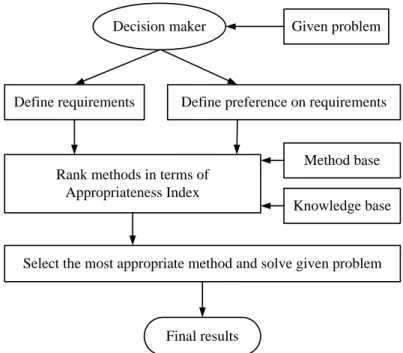
3.3 An Intelligent Multi-Criteria Decision Support System . . . 42
3.4 Chapter Summary . . . 43
4 Uncertainty Assessment in the Decision Analysis Process 45 4.1 Uncertainty Characterization . . . 45
4.1.1 Relationship Between Normal Distribution and Error Function . 46 4.1.2 Uncertainty Transformation using Inverse Error Function . . . . 46
4.2 Uncertainty Analysis . . . 47
4.2.1 Background of Error Propagation Techniques . . . 48
4.2.2 Robustness Measurement using Signal-to-Noise Ratio . . . 51
4.3 Local Sensitivity Analysis via Iterative Binary Search Algorithm . . . . 52
4.3.1 Iterative Binary Search Algorithm . . . 53
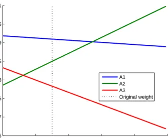
4.3.2 Interactive Sensitivity Analysis for Weighting Factors . . . 55
4.4 Global Sensitivity Analysis Using Partial Rank Correlation Coefficients 60 4.4.1 Correlation Coefficients and Statistical Significance Test . . . 60
4.4.2 Proposed Approach to Perform Global Sensitivity Analysis . . . 64
4.5 An Uncertainty Assessment Module . . . 68
CONTENTS
5 Proof of Concept 1: MCDA in Aircraft Design 71
5.1 Definition of the Decision Making Problem . . . 72
5.1.1 Identification of Design Criteria . . . 73
5.1.2 Parametric Studies of Design Criteria . . . 75
5.2 Selection of an Appropriate MCDA Method . . . 78
5.3 Proposed Multi-Criteria Optimization Framework . . . 83
5.3.1 Numerical Optimization Techniques . . . 83
5.3.2 Optimization Results of Typical Weighting Scenarios . . . 86
5.3.3 Comparison Using Different MCDA Indices as Objective Functions 89 5.4 Surrogate Model Construction for Design Criteria in terms of Weighting Factors . . . 92
5.4.1 Experimental Design . . . 93
5.4.2 Model Choice . . . 96
5.4.3 Model Fitting . . . 98
5.4.4 Model Validation . . . 98
5.5 Uncertainty Assessment for Weighting Factors via Surrogate Models . . 103
5.5.1 Uncertainty Characterization . . . 103
5.5.2 Uncertainty Analysis . . . 104
5.5.3 Sensitivity Analysis . . . 108
5.6 Discussion . . . 113
6 Proof of Concept 2: MCDA in Aircraft Evaluation 115 6.1 Definition of the Decision Making Problem . . . 115
6.1.1 Identification of Evaluation Criteria . . . 117
6.1.2 Quantification of Additional Soft Criteria . . . 117
6.2 Selection of an Appropriate MCDA Method . . . 124
6.3 Evaluation Results using ELECTRE I . . . 128
6.3.1 Stepwise Calculations of ELECTRE I . . . 128
6.3.2 Typical Weighting Scenarios for ELECTRE I . . . 132
6.4 Uncertainty Assessment . . . 133
6.4.1 Uncertainty Characterization . . . 133
6.4.2 Uncertainty Analysis . . . 135
CONTENTS
6.5 Discussion . . . 152
7 Conclusions 155 7.1 Research Questions Answered . . . 155
7.2 Summary of Scientific Contributions . . . 157
7.3 Recommendations . . . 158
References 159 A Preference Information Elicitation Techniques 165 A.1 Direct Assignment Method . . . 165
A.2 Eigenvector Method . . . 166
A.3 Entropy Method . . . 167
A.4 SMART . . . 168
A.5 Kano’s Model . . . 168
A.6 Distance-to-target Method . . . 169
B User Guide of an Intelligent Multi-Criteria Decision Support System171 B.1 Select the Most Appropriate Method . . . 172
B.2 Use Specific Method to Solve Given Problem . . . 176
B.3 Uncertainty Assessment . . . 176
C Additional Figures 179 C.1 Parametric Studies of Design Criteria . . . 179
C.2 Distributions of Design Criteria with Uncertainty Variation . . . 184
C.3 Interactive Weighting Plots for Business Aircraft Evaluation . . . 188
D Data Sources 193 D.1 Data for Surrogate Model Construction in terms of Weighting Factors . 193 D.2 Additional Untried Data for Evaluation of Surrogate Model Accuracy . 198 D.3 Typical Weighting Scenarios for Business Aircraft Evaluation . . . 203
List of Figures
1.1 Thesis Outline . . . 5
2.1 The Relationship Among Criteria, Attributes, and Objectives (73) . . . 8 2.2 Pareto Frontier in Two Dimensions . . . 10 2.3 Six Types of Generalized Criteria (16) . . . 24 2.4 TOPSIS Method (39) . . . 27 2.5 Pareto Frontier for the Relative Closeness to the Ideal Solutions in TOPSIS 29 2.6 Pareto Frontier for the Relative Closeness to the Ideal Solutions in the
Car Selection Example . . . 31
3.1 An Advanced Approach to MCDA Method Selection . . . 36 3.2 The Architecture of an Intelligent Multi-Criteria Decision Support System 42 4.1 Typical Numbers of Standard Deviation . . . 47 4.2 The Process of Uncertainty Analysis using Error Propagation Techniques 48 4.3 The Probabilistic Ranking Permutations in the Car Selection Example . 51 4.4 Initialization for the Iterative Binary Search Algorithm . . . 55 4.5 Flow Chart of the Iterative Binary Search Algorithm . . . 58 4.6 Interactive Sensitivity Analysis for the Weighting Factor of C1 in the
Car Selection Example . . . 59 4.7 The Input Variables and Output Variables in the Decision Analysis Process 60 4.8 Partial Rank Correlation Coefficients forA1 in the Car Selection Example 68 4.9 The User Interface of the Uncertainty Assessment Module . . . 69
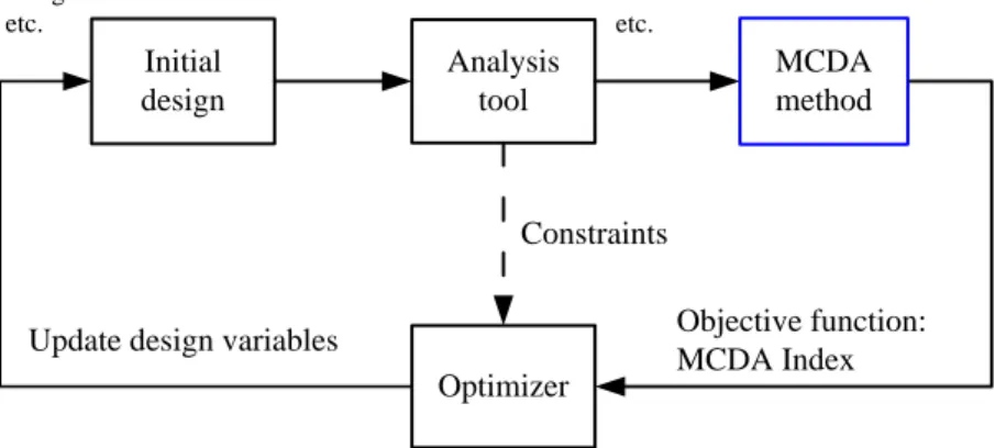
5.1 The Framework of Incorporating MCDA Techniques in Aircraft Design . 72 5.2 The Simplified Aircraft Mission Profile . . . 72
LIST OF FIGURES
5.3 Parametric Study of Thickness-to-chord Ratio versus OEM, Fuel Mass, Utilization/(Block time), Passenger Density, DOC, Aircraft Price, Fuel
Cost, and TOM . . . 76
5.4 Questions Related to Evaluation Criteria for Method Selection in Air-craft Design Process . . . 79
5.5 MCDA Methods Ranking List with Scores in Aircraft Design Process . . 80
5.6 Methodology Instructions for TOPSIS . . . 81
5.7 Comparison of Relative Changes for Design Criteria and Traced Perfor-mance Measures, using ITOPSIS Index and SAW Index as Objective Functions . . . 91
5.8 Overview of Surrogate Modeling Process for Design Criteria in terms of Weighting Factors . . . 92
5.9 Standard Latin Hypercube Sampling in Three Dimensions and with Two Dimensional Projections . . . 95
5.10 Normalized Latin Hypercube Sampling by Its Row Sum in Three Di-mensions and with Two Dimensional Projections . . . 96
5.11 Modified Latin Hypercube Sampling with Dirichlet Distribution in Three Dimensions and with Two Dimensional Projections . . . 97
5.12 The Actual by Predicted Plots of OEM, Fuel Mass, Utilization/(Block time), and Passenger Density, when using ITOPSIS Index as an Objec-tive Function . . . 99
5.13 The Actual by Predicted Plots of OEM, Fuel Mass, Utilization/(Block time), and Passenger Density, when using SAW Index as an Objective Function . . . 100
5.14 Histograms of Uncertainty Propagation for OEM, Fuel Mass, Utiliza-tion/(Block time), and Passenger Density . . . 105
5.15 Uncertainty Variation for OEM . . . 110
5.16 Robustness Comparison for Four Design Criteria . . . 111
5.17 The Prediction Profilers for Four Design Criteria . . . 112
6.1 The Specifications of Business Aircraft (2) . . . 118 6.2 Rating Scale of the Aviation International News 2010 Product Survey (80)120 6.3 Results of the Aviation International News 2010 Product Survey (80) . 120
LIST OF FIGURES
6.4 Questions Related to Evaluation Criteria for Method Selection in
Busi-ness Aircraft Evaluation Process . . . 125
6.5 MCDA Methods Ranking List in Business Aircraft Evaluation Process . 126 6.6 Methodology Instructions for ELECTRE I . . . 127
6.7 Nested Monte Carlo Simulation Loop for Confidence Quantification . . . 137
6.8 Interactive Sensitivity Analysis for Weighting Factors . . . 140
6.9 Interactive Weighting Plot for Criterion 1 . . . 141
6.10 Tornado Plots of Partial Rank Correlation Coefficients for the Four Al-ternatives using ELECTRE I, with Corresponding p-values . . . 150
6.11 Tornado Plots of Partial Rank Correlation Coefficients for the Four Al-ternatives using TOPSIS, with Corresponding p-values . . . 151
A.1 Attributes Classification in Kano’s Model (9) . . . 169
B.1 Main Interface of an Intelligent Multi-Criteria Decision Support System 171 B.2 Interface of Decision Maker Related Characteristics . . . 172
B.3 Summary of Decision Maker Related Characteristics . . . 172
B.4 Interface of Problem Related Characteristics . . . 173
B.5 Summary of Problem Related Characteristics . . . 174
B.6 Ranking of MCDA Methods with Appropriateness Scores . . . 175
B.7 Methodology Instructions for the Dominance Method . . . 175
B.8 Sixteen MCDA Methods List . . . 176
B.9 Interface of Uncertainty Assessment Module . . . 177
C.1 Parametric Study of Aspect Ratio versus OEM, Fuel Mass, Utiliza-tion/(Block time), Passenger Density, DOC, Aircraft Price, Fuel Cost, and TOM . . . 180
C.2 Parametric Study of Reference Area versus OEM, Fuel Mass, Utiliza-tion/(Block time), Passenger Density, DOC, Aircraft Price, Fuel Cost, and TOM . . . 181
C.3 Parametric Study of Cruise Mach Number versus OEM, Fuel Mass, Utilization/(Block time), Passenger Density, DOC, Aircraft Price, Fuel Cost, and TOM . . . 182
LIST OF FIGURES
C.4 Parametric Study of Fuselage Diameter versus OEM, Fuel Mass, Utiliza-tion/(Block time), Passenger Density, DOC, Aircraft Price, Fuel Cost,
and TOM . . . 183
C.5 Uncertainty Variation for Fuel Mass . . . 185
C.6 Uncertainty Variation for Utilization/(Block time) . . . 186
C.7 Uncertainty Variation for Passenger Density . . . 187
C.8 Interactive Weighting Plot for Criterion 2 . . . 189
C.9 Interactive Weighting Plot for Criterion 3 . . . 189
C.10 Interactive Weighting Plot for Criterion 4 . . . 190
C.11 Interactive Weighting Plot for Criterion 5 . . . 190
C.12 Interactive Weighting Plot for Criterion 6 . . . 191
C.13 Interactive Weighting Plot for Criterion 7 . . . 191
D.1 Histograms of One Hundred Sets of Weighting Factors Generated by Modified LHS with Dirichlet Distribution . . . 194
List of Tables
2.1 Typical Non-compensatory and Compensatory Decision Analysis
Meth-ods (39) . . . 7
2.2 Decision Matrix . . . 9
2.3 The Decision Matrix of a Car Selection Problem using ELECTRE I . . 15
2.4 Main Characteristics of ELECTRE Methods (68) . . . 17
2.5 Pairwise Comparison Scale (70) . . . 20
2.6 The Decision Matrix of a Car Selection Problem using TOPSIS . . . 30
3.1 The Appropriateness Index Calculation Process for TOPSIS . . . 40
4.1 The Decision Matrix of a Car Selection Problem for Uncertainty Analysis 50 4.2 The Probabilistic Ranking in the Car Selection Example . . . 50
4.3 Decision Matrix of a Car Selection Problem for Local Sensitivity Analysis 56 4.4 Absolute Minimum Changes in Weighting Factors to Alter the Rankings of Alternatives in the Car Selection Example . . . 57
4.5 Relative Minimum Changes in Weighting Factors to Alter the Rankings of Alternatives in the Car Selection Example . . . 57
4.6 The Decision Matrix of a Car Selection Problem for Global Sensitivity Analysis . . . 67
5.1 The Baseline and Ranges of Design Variables . . . 73
5.2 Summary of Design Variables, Constraints, and Design Criteria in Air-craft Optimization Process . . . 78
5.3 The Positive Ideal Solution and Negative Ideal Solution in ITOPSIS . . 82
5.4 Ten Sets of Random Starting Points in the Optimization Process . . . . 85
LIST OF TABLES
5.6 Optimization Results for Single Criterion . . . 86 5.7 Optimization Results when Weighting Factors are Evenly Distributed . 87 5.8 Optimization Results using SAW Index as an Objective Function, when
Weighting Factors are Evenly Distributed . . . 89 5.9 Comparison of Convergence Rates, using ITOPSIS Index and SAW Index
as Objective Functions . . . 90 5.10 Pairwise Correlation Coefficients for Design Criteria of Interest . . . 98 5.11 The Diagnostics of Response Surface Models for Design Criteria, using
ITOPSIS Index and SAW Index as Objective Functions . . . 101 5.12 Relative Errors Between Actual and Predicted Values for Design Criteria 102 5.13 Uncertainty Characterization for Weighting Factors . . . 103 5.14 Comparison of Design Criteria with Deterministic and Uncertain
Weight-ing Factors . . . 106 5.15 Uncertainty Variation for Weighting Factors, Regarding Percentage
Un-certainty and Confidence Level . . . 107
6.1 Segmentation Criteria for Business Jets (13) . . . 116 6.2 Ten Categories of the Aviation International News 2010 Product
Sur-vey (80) . . . 119 6.3 Four Categories of the Aviation Week’s 16th Annual Top-Performing
Companies Study (4) . . . 121 6.4 The Scores of the Six Major Business Jet Manufacturers (4) . . . 122 6.5 Ten Evaluation Criteria of Business Aircraft . . . 123 6.6 The Values of Evaluation Criteria for the Four Business Jet Alternatives 124 6.7 Evaluation Results for 84 Sets of Weighting Factors using ELECTRE I . 133 6.8 Uncertainty Characterization for Weighting Factors and Criteria Values 134 6.9 Three Scenarios for Uncertainty Analysis . . . 135 6.10 The Probabilistic Outranking Relationships in Three Scenarios . . . 136 6.11 The 95% Confidence Intervals for the Probabilistic Outranking
Relation-ship in Three Scenarios . . . 138 6.12 Absolute Minimum Changes in Weighting Factors to Alter the
LIST OF TABLES
6.13 Relative Minimum Changes in Weighting Factors to Alter the Non-dominance or Dominance Status of Alternatives . . . 139 6.14 Frequency of Status Change for Alternatives in Interactive Weighting Plots141 6.15 Physical Constraints of the Decision Criteria for Business Aircraft . . . 143 6.16 Absolute Minimum Changes in Criteria Values to Alter the Non-dominance
or Dominance Status of Alternatives . . . 144 6.17 Relative Minimum Changes in Criteria Values to Alter the Non-dominance
or Dominance Status of Alternatives . . . 145 6.18 Probability Distributions for Input Variables . . . 146 6.19 Comparison of Sensitivity Rankings for Input Variables Identified by
Local and Global Sensitivity Analysis . . . 154 A.1 Direct Assignment Method with a Ten-point Scale . . . 166 A.2 Random Consistency Index (RI)(70) . . . 167 D.1 One Hundred Sets of Weighting Factors Generated by Modified LHS
with Dirichlet Distribution and Design Criteria Values . . . 195 D.2 The 84 Sets of Weighting Factors and Predicted Design Criteria Values,
Obtained by the Analysis Tool (VAMPzero) . . . 199 D.3 Predicted Design Criteria Values for the 84 Data Points and Relative
Error(%), Generated by Surrogated Models . . . 201 D.4 The 84 Sets of Weighting Factors for Business Aircraft Evaluation, D:
Glossary
• ACJ: Airbus Corporate Jet
• AHP: Analytical Hierarchy Process
• AI: Appropriateness Index
• ANP: Analytical Network Process
• ATM: Air Traffic Management
• BBJ: Boeing Business Jet
• BCA: Business & Commercial Aviation
• CI: Consistency Index
• CL: Confidence Level
• CR: Consistency Ratio
• DLR: German Aerospace Center
• DM: Decision Maker
• DOC: Direct Operating Costs
• ELECTRE: Elimination and Choice Translation Reality
• EPNdB: Decibels of Effective Perceived Noise
• GA: Genetic Algorithms
LIST OF TABLES
• IFR: Instrument Flight Rules
• ITOPSIS: Improved TOPSIS
• LCA: Life Cycle Assessment
• LHS: Latin Hypercube Sampling
• MADM: Multi-Attribute Decision Making
• MCDA: Multi-Criteria Decision Analysis/Aid
• MCDM: Multi-Criteria Decision Making
• MODM: Multi-Objective Decision Making
• N/F: Non-Feasible
• NBAA: National Business Aviation Association
• OEM: Operating Empty Mass
• OR: Operational Research
• PN/F: Physically Non-Feasible
• PROMETHEE: Preference Ranking Organization METHod for Enrichment Eval-uations
• RI: Random Consistency Index
• RMSE: Root Mean Square Error
• SAW: Simple Additive Weighting
• SMART: Simple Multi-Attribute Rating Technique
• SNR: Signal-to-Noise Ratio
• TOM: Take-off Mass
• TOPSIS: Technique for Order Preference by Similarity to Ideal Solution
1
Introduction
The demands on air travel are increasing, not only regarding lower costs, but also better service quality, higher safety, and more environmental friendliness. The imperatives of air transport have evolved from Higher, Further, Faster to More Affordable, Safer, Cleaner and Quieter (1). In order to sustain the growth of air transport in a long term, the aerospace industry is faced with the challenge of designing more competitive aircraft satisfying these multiple criteria simultaneously.
As an important field in Operational Research (OR), Multi-Criteria Decision Anal-ysis (MCDA) is a process that allows one to make decisions in the presence of multiple, potentially conflicting criteria (87). Common elements in the decision analysis process are a set of design alternatives, multiple decision criteria, and weighting factors reflect-ing the preference information of Decision Maker (DM). The MCDA techniques can help the DM to evaluate the overall performance of the design alternatives. Further, the MCDA techniques can provide aiding in the generation, analysis, and optimization of design solutions.
1.1
Motivation
The competitiveness of an aircraft is no longer dominated by economic criteria, such as purchase price and operating costs (26). Moreover, it is alerted that by applying classic Direct Operating Costs (DOC) comparisons as the only yardstick in the evaluation of an aircraft, manufacturers run the risk of designing aircraft types and capabilities not fully suited to satisfy long term transportation needs (58).
1. INTRODUCTION
In addition to the economic consideration, there are several other criteria needed to be taken into account in aircraft design and evaluation decision making processes. For instance, environmental aspects and level of comfort. Continuous growth in passenger traffic and increasing public awareness of aircraft noise and emissions have made envi-ronmental considerations extremely critical in the design of future aircraft (5). Besides, passengers are more concerned about crowded flight and airlines are criticized for the increasing of load factors in order to fully utilized the capacity (76). Therefore, consid-ering these multiple criteria simultaneously, aircraft design and aircraft evaluation are typical multi-criteria decision making problems and need to be prudently conducted.
Applying the MCDA techniques in aircraft design and aircraft evaluation processes is one strategy to deal with multiple, conflicting criteria. The MCDA techniques are utilized to aggregate the multiple design criteria into one composite figure of merit, which serves as an objective function in the optimization process. The MCDA tech-niques allow transparent trade-offs among criteria and support the designer to quickly assess the compromised design alternatives. Moreover, the MCDA techniques have the ability to handle large number of criteria in the design and evaluation processes.
Theory of the MCDA Techniques
Although MCDA as a discipline has a relatively short history of about 40 years, over 70 MCDA techniques have been developed for facilitating the decision making pro-cess (87). Among these 70 MCDA techniques, different methods have different under-lying assumptions, information requirements, analysis models, and decision rules that are designed for solving a certain class of decision making problems. This implies that it is critical to select the most appropriate method to solve a given problem.
Decision criteria and weighting factors are main input data in the decision making process. It is observed that there are always uncertainties existing in the decision criteria due to incomplete information or limited knowledge, while the weighting factors are often highly subjective, considering the fact that they are elicited based on the DM’s experience or intuition (7), (28). Therefore, uncertainty assessment for the decision criteria and the weighting factors should be prudently performed.
1.1 Motivation
Practice of the MCDA Techniques in Aerospace Industry
Aerospace Systems Design Laboratory at Georgia Institute of Technology pioneered the application of the MCDA techniques in aerospace systems design. A probabilis-tic MCDA method for multi-objective optimization and product selection was devel-oped (6). However, it was pointed that this method did not consider the absolute location of the joint probability distribution and the weighting factors were used to adjust the target values (49). Technique for Order Preference by Similarity to Ideal Solution (TOPSIS) was utilized to the selection of technology alternatives in concep-tual and preliminary aircraft design (44). However, TOPSIS has the limitations that it assumes that each criterion’s utility is monotonic and is rather sensitive to the weight-ing factors. A multi-criteria interactive decision-makweight-ing advisor for the selection of the most appropriate decision making method was developed (48). However, only limited methods were implemented and the uncertainties propagated in the decision analysis process were not addressed explicitly.
Only limited research has been conducted to aircraft evaluation using the MCDA techniques. Four civil aircraft in terms of six criteria was evaluated by Simple Additive Weighting (SAW) (18). However, SAW is very sensitive to the normalization method and the weighting factors. Besides, civil aircraft was assessed by three criteria: DOC, operational commonality, and added values (58), (26). The added values were quanti-fied by equivalent DOC based on the weighting factors. However, inherent subjectivity and uncertainty of the weighting factors detriments the usefulness of this approach. Further, seven initial training aircraft were evaluated by sixteen criteria using TOP-SIS (82). However, only technical performance are considered because of the difficulty of collecting qualitative data. In addition, three MCDA methods: SAW, TOPSIS, and Analytic Hierarchy Process (AHP), were applied to an airport selection problem, where seven alternatives were evaluated by twelve criteria (40). The authors concluded that these three methods generated consistent result with the same weighting factors and suggested that the weighting factors should be considered more carefully.
In summary, although large efforts have been made to the application of the MCDA techniques, a large gap still exists between theory and practice, especially in the aerospace industry.
1. INTRODUCTION
1.2
Research Statement
The goal of this research is to fill the gap by investigating how existing MCDA tech-niques can be improved to better solve decision making problems, and how to imple-ment the improved MCDA techniques in aircraft design and evaluation processes. The following research objectives are considered critical to achieve the overall research goal:
1. Apply the most appropriate MCDA method for the decision making problem under consideration.
2. Assess the uncertainties propagated in the decision analysis process when applying the MCDA techniques.
3. Demonstrate the capabilities of the MCDA techniques with uncertainty assess-ment in aircraft design and aircraft evaluation processes.
The research objectives of this study can be best introduced through a series of research questions as follows:
• Question 1: How to select the most appropriate MCDA method for the decision making problem under consideration?
• Question 2: How to capture and assess the uncertainties propagated in the decision analysis process when solving decision making problems?
• Question 3: How to implement the MCDA techniques in aircraft design and aircraft evaluation processes?
In order to answer the research questions, several hypotheses are proposed:
• Hypothesis 1: It is feasible to quantify the appropriateness of the MCDA meth-ods for a given decision making problem. (Question 1)
• Hypothesis 2: Statistical techniques are capable of effectively dealing with the uncertainties propagated in the decision analysis process. (Question 2)
• Hypothesis 3: It is beneficial to implement the MCDA techniques in aircraft design and aircraft evaluation processes. (Question 3)
1.3 Thesis Outline
1.3
Thesis Outline
The outline of the thesis is illustrated in Figure 1.1. In Chapter 2, an overview of the MCDA techniques is provided. An advanced approach to facilitate the selection of the most appropriate MCDA method is presented and an intelligent multi-criteria decision support system is developed in Chapter 3. Chapter 4 introduces a new uncertainty assessment approach in the decision analysis process. In Chapter 5, the implementation of an improved MCDA technique with uncertainty assessment in aircraft design is presented as the first proof of concept. In Chapter 6, business aircraft evaluation using an appropriate MCDA technique with uncertainty assessment is presented as the second proof of concept. The thesis is summarized and some recommendations for future work are given in Chapter 7.
1. Introduction
5. Proof of Concept 1: MCDA in Aircraft Design
3. MCDA Method Selection
4. Uncertainty Assessment 2. MCDA Techniques
Overview
7. Conclusions
6. Proof of Concept 2: MCDA in Aircraft Evaluation
2
Multi-Criteria Decision Analysis
Techniques Overview
There are essentially two approaches to solve decision making problems: non-compensatory and compensatory methods (39). Non-compensatory methods do not permit trade-offs among criteria, while compensatory methods permit trade-offs among criteria. Accord-ing to this classification, several widely used decision analysis methods are summarized in Table 2.1 and will be explained in detail in the following sections.
Table 2.1: Typical Non-compensatory and Compensatory Decision Analysis Methods (39)
Non-compensatory Methods Compensatory Methods Conjunctive method Analytic hierarchy process Disjunctive method Expected utility theory Dominance method Multi-attribute utility theory
ELECTRE Multiplicative weighting method
Elimination by aspects PROMETHEE
Lexicographic method Simple additive weighting
Maximin method TOPSIS
Maximax method
It is noted that ELECTRE is classified as one non-compensatory method (14), considering that the role of criteria weights in ELECTRE are coefficients of impor-tance (68), (20). Besides, a poor criterion is judged irrespective to other good criteria, which distinguishes ELECTRE from compensatory methods (60).
2. MULTI-CRITERIA DECISION ANALYSIS TECHNIQUES OVERVIEW
2.1
Concepts and Terminologies
In order to have a universal understanding of the MCDA techniques, several important concepts and terminologies are introduced in this section.
MCDM and MCDA
There are two schools of decision analysis methods: Multi-Criteria Decision Making (MCDM) developed by the American school (85), and Multi-Criteria Decision Analy-sis/Aid (MCDA) created by the European school (67). Most researchers use MCDM and MCDA interchangeably (7), (87), (28). In this research, the European school (MCDA) is followed.
Criteria, Attributes, and Objectives
The distinctions among criteria,attributes, and objectives are made as follows (39).
• Criteria: A criterion is a measure of performance when evaluating an alternative.
• Attributes: An attribute is an inherent characteristic of an alternative.
• Objectives: An objective is something to be pursued to its fullest. It indicates the direction of change desired.
The relationship amongcriteria,attributes, and objectives are shown in Figure 2.1. Criteria Attributes (Selection) Objectives (Design) With direction
Figure 2.1: The Relationship Among Criteria, Attributes, and Objectives (73)
As shown in Figure 2.1, criteria are emerging as a form of attributes or objectives, and attributes with directions are objectives. For example, level of comfort is a criterion when evaluating an aircraft, cabin volume and noise are attributes of the aircraft which can be used to measure the level of comfort, the maximization of cabin volume and the minimization of noise are objectives in the aircraft design process.
2.1 Concepts and Terminologies
Decision Matrix
At the heart of the MCDA techniques is the concept of decision matrix. LetAi be the i-th alternative (i= 1,2, ..., m) and xj be the j-th criterion (j = 1,2, ..., n). Suppose
xij stands for the value of criterion xj with respect to alternativeAi. Then, a quanti-tative MCDA problem of ranking or sortingm alternatives based on n criteria can be represented using decision matrix, as shown in Table 2.2.
Table 2.2: Decision Matrix
Alternatives Criteria A1 x11 x12 . . . x1n A2 x21 x22 . . . x2n .. . ... ... . .. ... Am xm1 xm2 . . . xmn Preference Information
The preference information describes the DM’s attitude in favor of one criterion over another when choosing between alternatives, usually in the form of weighting factors. Typical preference information elicitation techniques can be found in Appendix A.
Pareto Frontier
Pareto frontier is introduced to find the best compromised solution which has the maximum overall performance satisfying all the criteria simultaneously (38). In the feasible solution space, a solution is dominated if there is another solution which excels it in one or more criteria and equals it in the remainder (17). A non-dominated solution is one which no criteria can be improved without a simultaneous detriment to at least one of the others. A two-dimensional Pareto frontier for the minimization of two criteria is illustrated in Figure 2.2. It can be seen that Pareto frontier is composed of non-dominated solutions.
With these important concepts and terminologies, several typical decision analysis methods will be introduced in the following sections.
2. MULTI-CRITERIA DECISION ANALYSIS TECHNIQUES OVERVIEW
Figure 2.2: Pareto Frontier in Two Dimensions
2.2
Typical Non-compensatory Decision Analysis
Meth-ods
Non-compensatory decision analysis methods do not permit trade-offs between crite-ria, that is, a disadvantage in one criterion cannot be offset by an advantage in other criterion. The non-compensatory methods are credited for their simplicity. As summa-rized in Table 2.1, typical non-compensatory decision analysis methods are explained in detail in the following subsections.
2.2.1 Conjunctive Method
The DM sets up the acceptable minimal criteria values. Any alternative which has a criterion value less than the standard level will be rejected (39). The i-th alternative
Ai (i= 1,2, ..., m) is classified as an acceptable alternative only if
xij ≥x0j, j= 1,2, ..., n (2.1) where x0j is the standard level of the j-th criterion xj, and bigger criteria values are preferred. The cutoff values given by the DM play a key role in eliminating the alterna-tives; if too high, none is left; if relatively low, several alternatives are left after filtering. Hence increasing the minimal standard levels in an iterative way, the alternatives can be narrowed down to a single choice.
2.2 Typical Non-compensatory Decision Analysis Methods
The Conjunctive method does not require the criteria to be in numerical form, and the relative importance of the criteria is not needed. The Conjunctive method is not usually used for selection of alternatives but rather for dichotomizing them into acceptable and not acceptable categories.
2.2.2 Disjunctive Method
In the Disjunctive method, an alternative is evaluated on its greatest value of a crite-rion (39). The i-th alternativeAi (i= 1,2, ..., m) is classified as an acceptable alterna-tive only if
xij ≥x0j, j= 1 or 2 or...orn (2.2) where x0j is the desirable level of the j-th criterion xj, and bigger criteria values are preferred.
As with the Conjunctive method, the Disjunctive method does not require the criteria to be in numerical form, and it does not need information on the relative importance of the criteria.
2.2.3 Dominance Method
In order to obtain a set of non-dominated solutions before the final choice, the Dom-inance method can be used to screen the alternatives. The DomDom-inance method takes the following procedures (17) :
• Compare the first two alternatives and if one is dominated by the other, discard the dominated one.
• Next, compare the un-discarded alternative with the third alternative and discard any dominated alternative.
• Then, compare the fourth alternative and so on.
• After all the alternatives are compared, the non-dominated set is determined.
The Dominance method does not require any assumption or any transformation of criteria. The non-dominated set usually has multiple alternatives, hence, the Domi-nance method is mainly used for initial filtering.
2. MULTI-CRITERIA DECISION ANALYSIS TECHNIQUES OVERVIEW
2.2.4 ELECTRE
ELECTRE (Elimination and Choice Translation Reality) methods use the concept of outranking relation introduced by Benayoun (8). For instance, suppose there are m
alternatives based on n evaluation criteria, with weighting factors [w1, w2, ..., wn], xij stands for the value of criterion xj with respect to alternative Ai. An outranking relation between alternative Ak and alternative Al (k, l = 1,2, ..., m, k 6= l) is defined as: Ak is preferred to Al when Ak is at least as good as Al with respect to a majority of criteria and when Ak is not significantly poor regarding any other criteria. After the assessment of the outranking relations for each pair of alternatives, dominated alternatives can be eliminated and non-dominated alternatives can be obtained for further consideration.
There are several different versions of ELECTRE methods, including ELECTRE I, IS, II, III, IV and TRI (68), (21). ELECTRE I is the first decision analysis method using the concept of outranking relation, the other versions of ELECTRE methods are extensions of ELECTRE I. In this subsection, the stepwise calculations of ELECTRE I will be described in detail and the other ELECTRE methods will be briefly introduced. ELECTRE I is composed of the following nine steps (39).
1. Normalize the decision matrix
R= r11 r12 ... r1n r21 r22 ... r2n .. . ... . .. ... rm1 rm2 ... rmn , rij = xij s m P i=1 x2ij , i= 1,2, ..., m, j= 1,2, ..., n (2.3)
2. Calculate the weighted normalized decision matrix.
V =RW = r11 r12 ... r1n r21 r22 ... r2n .. . ... . .. ... rm1 rm2 ... rmn w1 w2 . .. wn (2.4)
2.2 Typical Non-compensatory Decision Analysis Methods
For each pair of alternatives Ak and Al, the set of decision criteria J = (j |j = 1,2, ..., n) is divided into two disjoint subsets. The concordance set Ckl of Ak and Al is composed of all criteria which support thatAk is preferred toAl. The discordance set Dkl is the complementary subset of the concordance set Ckl. In other words, Dkl=J−Ckl.
Ckl={j|xkj ≥xlj},(k, l= 1,2, ..., m,andk6=l)
Dkl={j|xkj < xlj}=J−Ckl
(2.5)
4. Calculate the concordance matrixC.
The concordance index is calculated by the sum of the criteria weights which are contained in the concordance set. For example, the concordance index ckl between Ak and Al is calculated by Equation 2.7.
C = − c12 ... c1n c21 − c23 c2n .. . ... . .. ... cm1 cm2 ... − (2.6) ckl= P j∈Ckl wj n P j=1 wj (2.7)
5. Calculate the discordance matrixD.
The discordance index reflects the degree to which one alternative is worse than the other. For instance, the discordance indexdklbetweenAkandAlis calculated by Equation 2.9. D= − d12 ... d1n d21 − d23 d2n .. . ... . .. ... dm1 dm2 ... − (2.8) dkl = max j∈Dkl |vkj−vij| max j∈J |vkj−vij| (2.9)
2. MULTI-CRITERIA DECISION ANALYSIS TECHNIQUES OVERVIEW
It should be noticed that differences among criteria weights are contained in the concordance matrixC, while differences among criteria values are reflected in the discordance matrixD.
6. Determine the concordance dominance matrix.
A concordance threshold c needs to be chosen to perform the concordance test. Alternative Ak possibly dominates alternative Al, if the concordance index ckl exceeds at least a certain thresholdc, that is,ckl≥c.
In ELECTRE I, a Boolean matrix is used to convert the concordance test into numerical values (0 and 1). If the concordance test is passed (ckl≥c), then the concordance index is 1. Otherwise, if the concordance test is failed (ckl< c), the concordance index is 0.
7. Determine the discordance dominance matrix.
A discordance threshold d needs to be chosen to perform the discordance test. Alternative Ak possibly dominates alternative Al, if the discordance index dkl is smaller than a certain threshold d, that is, dkl≤d.
As with the case of the determination of the concordance dominance matrix, the discordance test is converted into numerical values (0 and 1) by a Boolean matrix. The discordance index is 1 when the discordance test is passed (dkl ≤d), and it is 0 when the discordance test is failed (dkl > d).
8. Aggregate the dominance matrix.
An outranking relation can be justified only if both the concordance index and the discordance index do not violate their corresponding thresholds. That is,ckl≥c and dkl ≤ d. The aggregated dominance matrix is calculated by an element-to-element product of the concordance dominance matrix and the discordance dominance matrix.
9. Eliminate the dominated alternatives.
The aggregated dominance matrix gives the partial preference of the alternatives. In the aggregated dominance matrix, the element 1 in the column indicates that this alternative is dominated by other alternatives. Thus, any alternative which has at least one element of 1 in the column can be eliminated.
2.2 Typical Non-compensatory Decision Analysis Methods
ELECTRE I is widely used because of its simple logic and refined computational procedures. However, the two concordance and discordance threshold values have sig-nificant impact on the final results. Additionally, the calculation procedures will become more complex as the increase of the dimension of decision matrix.
One Example of a Car Selection Problem using ELECTRE I
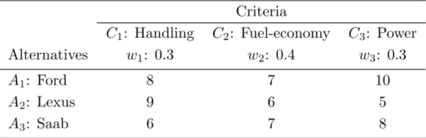
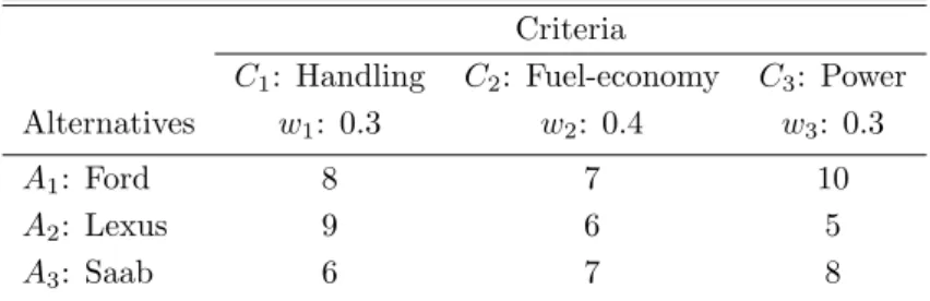
One example of a car selection problem using ELECTRE I is demonstrated in this subsection. Suppose that one DM wants to select a car with the consideration of three criteria: handling, fuel-economy, and power. Fuel-economy is one cost criterion (smaller value of fuel-economy is preferred), while handling and power are benefit criteria (big-ger values of handling and power are preferred). There are three alternatives available: Ford, Lexus, and Saab. A ten-point score is assigned to the three criteria for each al-ternative, respectively. The weighting factors among the three criteria are [0.3 0.4 0.3]. The decision matrix is summarized in Table 4.6.
Table 2.3: The Decision Matrix of a Car Selection Problem using ELECTRE I
Criteria
C1: Handling C2: Fuel-economy C3: Power Alternatives w1: 0.3 w2: 0.4 w3: 0.3
A1: Ford 8 7 10
A2: Lexus 9 6 5
A3: Saab 6 7 8
Given the decision matrix shown in Table 4.6, going through the described nine-step calculations of ELECTRE I, the aggregated dominance matrix is shown in matrixM.
In the aggregated dominance matrixM, the element 1 in the column indicates that this alternative is dominated by other alternatives. Thus,A3 is dominated by A1 and
2. MULTI-CRITERIA DECISION ANALYSIS TECHNIQUES OVERVIEW
car selection problem using ELECTRE I,A3 (Saab) should be eliminated from the can-didate cars,A1 (Ford) andA2 (Lexus) can be recommended for further consideration.
ELECTRE IS
ELECTRE IS is similar to ELECTRE I, except that in Step 6 (Determine the concor-dance dominance matrix), interval values between 0 and 1 are used instead of Boolean numbers (0 or 1) (68), (21), (60). In order to discriminate between two alternatives, two thresholds have to be defined for each criterion: indifference threshold and strict preference threshold.
ELECTRE II
ELECTRE II is also similar to ELECTRE I. The main difference lies in the definition of two outranking relations: strong outranking and weak outranking. For each criterion, two strong outranking thresholds and one weak outranking threshold have to be defined.
ELECTRE III
ELECTRE III uses the same principle of ELECTRE II. For each criterion, an indiffer-ence threshold, a preferindiffer-ence threshold, and a veto threshold have to be defined in order to compare the alternatives. Both the concordance dominance matrix and discordance dominance matrix are constructed by interval values between 0 and 1. The aggregation of the concordance dominance matrix and discordance dominance matrix is obtained by a credibility matrix. The final classification of alternatives is based on ascending and descending distillations (68), (21).
ELECTRE IV
Unlike the previously described ELECTRE methods, ELECTRE IV does not require criteria weights in the calculation procedures. Instead, it uses the number of criteria in different preference areas. For each criterion, an indifference threshold, a preference threshold, and a veto threshold are required in order to compare the alternatives. Similar to ELECTRE III, a credibility matrix is calculated, and the classification of alternatives is based on ascending and descending distillations.
2.2 Typical Non-compensatory Decision Analysis Methods
ELECTRE TRI
In ELECTRE TRI, some reference alternatives are introduced, all alternatives are compared to these reference alternatives. Similar to ELECTRE III, a credibility matrix is computed with respect to reference alternatives. The outranking relations between candidate alternatives and reference alternatives are established using the credibility matrix and a veto threshold. ELECTRE TRI can reduce the computational cost of alternative comparisons when the number of alternatives is large.
Summary of ELECTRE Methods
The main characteristics of all versions of ELECTRE methods were summarized by Roy (68), as shown in Table 2.4. Considering different problem statements, some guide-lines on how to choose among ELECTRE methods were also suggested. For instance, if it is truly essential to work with a very simple method and it is realistic to have no information on the indifference threshold and preference threshold, ELECTRE I should be selected in order to eliminate the non-dominated alternatives, while ELECTRE II should be used in order to build a partial pre-order of alternatives. ELECTRE VI would be convenient only if there exists a good reason to refusing the introduction of importance coefficients. In general, ELECTRE IS, II, III, IV, and TRI do provide powerful support for the classification of the alternatives. However, they require too many threshold definitions from DMs, thus, it is rather complex to implement these methods in real world problems (60).
Table 2.4: Main Characteristics of ELECTRE Methods (68)
ELECTRE methods I IS II III IV TRI
Require indifference no yes no yes yes yes
and preference thresholds
Require criteria weights yes yes yes yes no yes Outranking relations binary binary strong interval strictly, weakly, interval
and weak values hardly preferred, values or indifferent
2. MULTI-CRITERIA DECISION ANALYSIS TECHNIQUES OVERVIEW
2.2.5 Elimination By Aspects Method
In this method, the DM is assumed to have minimum cutoffs for each criterion. A criterion is selected, and all alternatives which do not pass the cutoff on that criterion are eliminated. Then another criterion is selected, and so forth. The process continues until all alternatives but one are eliminated (39).
The elimination by aspects method eliminates alternatives which do not satisfy some standard level, and it continues until all alternatives except one have been eliminated. However, only small part of the information is used when comparing the alternatives.
2.2.6 Lexicographic Method
In the Lexicographic method, the DM compares the alternatives on the most impor-tant criterion. If one alternative has a better criterion value than any of the other alternatives, the alternative is chosen and the decision process ends. However, if some alternatives are tied on the most important criterion, the subset of tied alternatives is then compared on the next most important criterion. The process continues sequen-tially until a single alternative is chosen or until all the criteria have been considered.
The Lexicographic method does not require comparability across criteria, and the preference information on the criteria is not necessarily in numerical values. However, it only utilizes a small part of the available information in making a final decision.
2.2.7 Maximin Method
In the Maximin method, the overall performance of an alternative is determined by the weakest or poorest criterion. The DM examines the criteria values for each alternative, note the worst value for each alternative, and then select the alternative with the most acceptable value in its worst criterion. It is the selection of the maximum (across alternatives) of minimum (across criteria) values, or the maximin (39). Mathematically speaking, the alternativeA∗ is selected such that
A∗ = Ai max i minj rij , i= 1,2, ..., m, j= 1,2, ..., n (2.10) whererij are normalized criteria values, and bigger criteria values are preferred.
2.3 Typical Compensatory Decision Analysis Methods
2.2.8 Maximax Method
In contrast to the Maximin method, the Maximax method selects an alternative by its best criterion value rather than its worst criterion value. In this method, the best cri-terion value for each alternative is identified, then these maximum values are compared in order to select the alternative with the best value (39). Mathematically speaking, the alternativeA∗ is selected such that
A∗ = Ai max i maxj rij , i= 1,2, ..., m, j= 1,2, ..., n (2.11)
whererij are normalized criteria values, and bigger criteria values are preferred. The Maximin method and the Maximax method are widely used in game theory. However, they utilize only a small part of the available information in making a final choice (only one criterion per alternative). The applicability of the Maximin method and the Maximax method is relatively limited.
2.3
Typical Compensatory Decision Analysis Methods
Compensatory decision analysis methods permit trade-offs between criteria, that is, small changes in one criterion can be offset by opposing changes in any other criteria. As summarized in Table 2.1, typical compensatory decision analysis methods are explained in detail in the following subsections.
2.3.1 Analytic Hierarchy Process
Analytic Hierarchy Process (AHP) was proposed to deal with decision making prob-lems that have hierarchical structures of attributes (70). AHP is based on the idea of translating the hierarchy problem to a series of pairwise comparison matrices and obtaining the preference information for the attributes using eigenvector method. As one popular preference information elicitation techniques, the eigenvector method is explained in Appendix A.2. The first part of this subsection introduces the pairwise comparison matrix, followed by the computational steps of AHP.
2. MULTI-CRITERIA DECISION ANALYSIS TECHNIQUES OVERVIEW
Pairwise Comparison Matrix
The pairwise comparison concept originated from an experiment considering the subject of stimuli and responses performed by Weber in 1846. Weber stated that change in sensation was noticed when the stimulus was increased by a constant percentage of the stimulus itself. A nine-point scale based on Weber’s law was created and shown in Table 2.5.
Table 2.5: Pairwise Comparison Scale (70)
Intensity of importance
Definition Explanation
1 Equal importance Two activities contribute equally to the objective. 3 Moderate importance of one
over another
Experience and judgment slightly favor one activity over another.
5 Strong importance Experience and judgment strongly favor one activity over another.
7 Very strong or demonstrated importance
An activity is favored very strongly over another; its dominance demonstrated in practice.
9 Extreme importance The evidence favoring one activity over another is of the highest possible order of affirmation. Reciprocals
of above
If activity i has one of the above nonzero numbers as-signed to it when compared with activity j, then j has the reciprocal value when compared withi.
A reasonable assumption.
Suppose there are m alternatives and n criteria in a given problem. A pairwise comparison matrix is ambymmatrix, whose elementyij indicates the DM’s preference information of alternativeiover alternative j for a given criterion. In total, there will ben m×m comparison matrices, as shown in Equation 2.12.
M = 1 y12 ... y1m y21 1 ... y2m .. . ... . .. ... ym1 ym2 ... 1 (2.12)
Computational Steps of AHP
2.3 Typical Compensatory Decision Analysis Methods
2. Formulate the pairwise comparison matrix, as shown in Equation 2.12, for ele-ments at a single level of the hierarchy with respect to each of the eleele-ments at a level immediately above.
3. Generate the weights of elements using the eigenvector method, as described in Appendix A.2. This procedure is repeated until all the weights of elements are obtained.
4. The alternative with a larger relative value is more favorable.
AHP provides a simple way to formulate a decision making problem and to elicit preference information, as it only requires pairwise comparisons between criteria or al-ternatives. However, it has some limitations. The preference independence among all elements at any level except for the bottom level is assumed. It would be problematic to use AHP where the criteria at the same level have correlated dependence. Another limitation in AHP is that the pairwise comparison matrix is required with each element describing the relative importance of an criterion over all other criteria or the relative preference of an alternative over all other alternatives. The complete pairwise compar-ison is not a trivial task for the DM and may trigger inconsistency problems, which will become worse with the increasing dimension of the pairwise comparison matrix.
2.3.2 Expected Utility Theory
Expected utility can be dated back to Daniel Bernoulli’s resolution to the St. Petersburg paradox in 1738 (22), (25). The rule of the St. Petersburg game is that the player tosses a fair coin untilhead shows up for the first time, if this occurs at k-th toss, the payoff is 2k guilders. The expected monetary value is
n P i=1
(12)k2k= 1 + 1 + 1 +...=∞. The people were asked how much they would pay for the game? However, the paradox is that no reasonable people would want to pay even small amount of money for the game with infinite expected value.
Bernoulli used a logarithmic utility index defined over wealth to compute a finite price for a gamble with an unbounded expected value, with the argumentation that the people estimate the game in terms of the utility of money outcomes, and the marginal utility is diminishing. For a person with present wealth a, the expected utility of the
2. MULTI-CRITERIA DECISION ANALYSIS TECHNIQUES OVERVIEW
game is calculated by Equation 2.13 (25).
X i
pilog(a+xi) (2.13)
wherepi is the probability of the i-th game, andxi is the outcome of the i-th game. The value of the game with fixed amountvis calculated by log(a+v) =P
i
pilog(a+
xi) and is shown in Equation 2.14 (25)
v=Y i
(a+xi)pi−a (2.14)
Expected utility theory state that the DM chooses between risky prospects by com-paring their expected utility values, which are calculated by the weighted sum of utility values of outcomes multiplied by their probabilities, as shown in Equation 2.15.
E(u|p, X) = X x∈X
p(x)u(x) (2.15)
where x is a particular outcome from the set of all possible outcomes X, p(x) is the probability of the particular come,u(x) is its utility function.
Expected utility theory is suitable for decision making problems with risk and uncer-tainty. However, it is difficult to obtain an accurate utility function for each criterion, and the consistency of the utility functions among different criteria is hard to maintain.
2.3.3 Multi-Attribute Utility Theory
This method is based on the concept of utility function, which represents a mapping from the DM’s preference into a mathematical function (43). The most widely used form is the additive multi-attribute utility method given by Equation 2.16, with two assumptions stating that the utility functions of all the attributes are independent and the relative weight of an attribute can be determined regardless of the relative weights of other attributes. U(x1, x2, ..., xn) = n X i=1 wiui(xi) (2.16)
where [w1, w2, ..., wn]Tare weighting factors,ui(xi) is the corresponding utility function of the i-th attribute xi .
2.3 Typical Compensatory Decision Analysis Methods
The additive multi-attribute utility provides utility function to represent the DM’s preference information. However, the two assumptions including the independence of utility function and weights do not hold true for many practical decision making problems, which limits the use of this method.
2.3.4 Multiplicative Weighting Method
In this method, the relative weights [w1, w2, ..., wn]T are assigned to the criteria by the DM, the criterion values for each alternative are multiplied, with the relative weights as exponents. This method chooses the most preferred alternative which has the biggest value, as shown in Equation 2.17, when bigger criteria values are preferred.
A∗= Ai max i n Y j=1 xwj ij , i= 1,2, ..., m, j= 1,2, ..., n (2.17)
Considering the exponentiation property, all criteria values should be greater than one in order to assure its monotonicity. When the criterion values are smaller than one, 10kshould be multiplied to all criterion values, wherekis an exponent which make the smallest criterion value bigger than one.
2.3.5 PROMETHEE
In PROMETHEE (Preference Ranking Organization METHod for Enrichment Evalu-ations) method (15), (16), a valued preference relationship based on a generalization of the notion of criteria is constructed first, and a preference index is defined and a val-ued outranking graph is obtained. According to the preference index, PROMETHEE I provides a partial preorder and PROMETHEE II offers a complete preorder on all actions (alternatives).
Criteria Generalization
The definition of the valued preference relationship between two actions a and b is described as follows (16):
• P(a, b) = 0 means an indifference betweenaand b.
2. MULTI-CRITERIA DECISION ANALYSIS TECHNIQUES OVERVIEW
• P(a, b)≈1 means strong preference ofaoverb.
• P(a, b) = 1 means strict preference ofaoverb.
For each criterion, a generalized criterion and a corresponding preference function are considered. In PROMETHEE, six types of generalized criteria are provided, as illustrated in Figure 2.3, whered is the difference between two criteria,p is the strict preference threshold, and q is the indifference threshold,sis the standard deviation in Gaussian distribution.
2.3 Typical Compensatory Decision Analysis Methods
Multi-Criteria Preference Index
The multi-criteria preference index of action a over action b, denoted by Π(a, b), is defined as in Equation 2.18 Π(a, b) = n P i=1 wiPi(a, b) n P i=1 wi (2.18)
wheren is the number of criteria, wi is the weighting factor of the i-th criterion, and
Pi is the preference function of the i-th criterion. The multi-criteria preference index ranges from 0 to 1, with Π(a, b)≈0 represents a weak preference of actionaover action
b, and Π(a, b)≈1 represents a strong preference of actionaover actionb.
PROMETHEE Rankings
A positive outranking flow is defined by Equation 2.19 and a negative outranking flow is defined by Equation 2.20, respectively. Besides, a net outranking flow is calculated by Equation 2.21. Φ+(a) =X b∈A Π(a, b) (2.19) Φ−(a) =X b∈A Π(b, a) (2.20) Φ(a) = Φ+(a)−Φ−(a) (2.21)
Based on Equation 2.19 and Equation 2.20, PROMETHEE I provides a partial preorder by considering the intersection of the positive outranking flow and negative outranking flow, which is listed as follows.
• Action aoutranks action b, if Φ+(a)≥Φ+(b) and Φ−(a)≤Φ−(b).
• Action ais indifferent from actionb, if Φ+(a) = Φ+(b) and Φ−(a) = Φ−(b).
2. MULTI-CRITERIA DECISION ANALYSIS TECHNIQUES OVERVIEW
Based on Equation 2.21, PROMETHEE II considers action a outranks action b if Φ(a)>Φ(b), and actionais indifferent from action bif Φ(a) = Φ(b).
The six types of preference function and the partial or complete preorder in PROMETHEE provides the DM more insights in solving the given problem. However, in order to de-fine the preference function, it requires too many threshold parameters. Moreover, these threshold parameters are rather subjective and different DMs often have different threshold values, which increases the complexity of the problem significantly.
2.3.6 Simple Additive Weighting
In Simple Additive Weighting (SAW) method (39), the relative weights [w1, w2, ..., wn]T are assigned to the criteria by the DM. The multiple criteria values together with their corresponding weights are aggregated into a single performance metric. SAW chooses the most preferred alternative A∗ which has the maximum weighted average outcome, as shown in Equation 2.22, when bigger criteria values are preferred.
A∗ = Ai max i n X j=1 wjxij , i= 1,2, ..., m, j= 1,2, ..., n (2.22)
SAW is one of the most widely known decision analysis methods because of its simplicity to understand and use. However, it also has some disadvantages. SAW requires all the criterion values to be both numerical and comparable, which will trigger the quantification problem of the qualitative criteria and normalization problem of all the elements in decision matrix. The quantification methods and normalization methods will have a significant influence on the final decision results. Moreover, SAW is sensitive to the weighting factors.
2.3.7 TOPSIS
TOPSIS (Technique for Order Preference by Similarity to Ideal Solution) is based on the idea that the chosen alternative should have the shortest distance to the positive ideal solution and the furthest distance from the negative ideal solution. The distance is in the form of Euclidean distance (39), as shown in Figure 2.4.
TOPSIS requires decision matrix and relative weights as input data, its computa-tional steps are summarized as follows.
2.3 Typical Compensatory Decision Analysis Methods
Figure 2.4: TOPSIS Method (39)
1. Normalize the decision matrix.
zij = xij s m P i=1 x2 ij , i= 1,2, ..., m, j= 1,2, ..., n (2.23)
2. Calculate the weighted normalized decision matrix.
rij =wjzij, i= 1,2, ..., m, j= 1,2, ..., n (2.24)
3. Identify the positive ideal solutionA∗ and the negative ideal solutionA−.
A∗ = max i rij|j ∈J , min i rij|j∈ ˆ J |i= 1,2, ..., m ={x∗1, x∗2, ..., x∗n} (2.25) A− = min i rij|j∈J , max i rij|j ∈ ˆ J |i= 1,2, ..., m = x−1, x−2, ..., x−n (2.26) where J is the benefit criteria set (bigger criterion value is preferred), and ˆJ
is the cost criteria set (smaller criterion value is preferred). Thus, the positive ideal solution is composed of the maximum values of benefit criteria and the
2. MULTI-CRITERIA DECISION ANALYSIS TECHNIQUES OVERVIEW
minimum values of cost criteria; while the negative ideal solution is composed of the minimum values of benefit criteria and the maximum values of cost criteria. 4. Calculate the distance of each alternative to the positive ideal solution and the
negative ideal solution, respectively.
Si∗= v u u t k X j=1 rij−x∗j 2 , i= 1,2, ..., m (2.27) Si−= v u u t k X j=1 rij−x−j 2 , i= 1,2, ..., m (2.28)
5. Calculate the relative closeness of each alternative to the ideal solutions.
Ci∗ = S − i
Si−+Si∗, i= 1,2, ..., m (2.29)
6. Rank the alternatives according to the value ofCi∗ .
TOPSIS suggests the best alternative which has the furthest distance from the negative ideal solution (biggest value ofSi−) and shortest distance to the positive ideal solution (smallest value of S∗i), thus, the increase of numerator and the decrease of denominator will lead to a bigger value of Ci∗ in Equation 2.29. In other words, the alternative which maximizes the value of Ci∗ ranks first.
Furthermore, in addition to Equation 2.29, the relative closeness of each alternative to the ideal solutions could be also aggregated by Equation 2.30.
Ci−= S ∗ i
Si∗+Si−, i= 1,2, ..., m (2.30)
where the decrease of numerator and the increase of denominator will result in a smaller value of Ci−. Thus, the alternative which minimizes the value ofCi− ranks first.
Besides, it is interesting to notice that the relationship between Equation 2.29 and Equation 2.30.
Ci∗+Ci−= 1, i= 1,2, ..., m (2.31) Another approach is to visualize the relative closeness of each alternative to the ideal solutions via Pareto frontier, as illustrated in Figure 2.5, where the horizontal
2.3 Typical Compensatory Decision Analysis Methods
coordinate represents the distance to the positive ideal solution (Si∗), while the vertical coordinate stands for the distance to the negative ideal solution with minus signal (−Si−). The minus signal is used to convert the preference direction of Si− for the convenience of displaying Pareto frontier.
1 -1 -0.75 -0.5 -0.25 0 0.25 0.5 0.75 0 Pareto frontier
Distance to Positive Ideal Solution
D is ta n ce t o N eg at iv e Id ea l S o lu ti o n
Figure 2.5: Pareto Frontier for the Relative Closeness to the Ideal Solutions in TOPSIS
The Pareto frontier approach does not need to aggregate the relative closeness to the ideal solutions, however, instead of one best alternative, a set of non-dominated alternatives are often obtained.
TOPSIS is one of the widely used compensatory decision analysis methods con-sidering its simplicity and systematic calculation procedures. However, it has some limitations. TOPSIS assumes that each criterion’s utility is monotonic, which is not ap-propriate for problems where a particular criterion value is desired to be achieved (39). TOPSIS is also rather sensitive to the weighting factors.
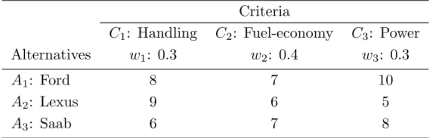
One Example of a Car Selection Problem using TOPSIS
In this subsection, TOPSIS is used to solve a car selection problem, as described in Subsection 2.2.4. The decision matrix shown in Table 4.6 is repeated here for the convenience of calculation.
2. MULTI-CRITERIA DECISION ANALYSIS TECHNIQUES OVERVIEW
Table 2.6: The Decision Matrix of a Car Selection Problem using TOPSIS
Criteria
C1: Handling C2: Fuel-economy C3: Power Alternatives w1: 0.3 w2: 0.4 w3: 0.3
A1: Ford 8 7 10
A2: Lexus 9 6 5
A3: Saab 6 7 8
six-step calculations of TOPSIS, the relative closeness aggregated by Equation 2.29 is shown in C∗. Considering that the alternative which maximizes the value ofC∗ ranks first, thus, A1 (Ford) is recommended as the best alternative for the DM.
C∗ = 0.5175 0.4866 0.5043
Furthermore, the relative closeness aggregated by Equation 2.30 is shown in C−. In this case, the alternative which has the smallest value of C− ranks first. Therefore,
A1 (Ford) is ranked as the best alternative for the DM.
C−= 0.4825 0.5134 0.4957
The Pareto frontier for the relative closeness to the ideal solutions is illustrated in Figure 2.6. It can be observed thatA1 (Ford) is the non-dominated alternative.
In summary, in this car selection example using TOPSIS, three approaches of rep-resenting the relative closeness of each alternative to the ideal solutions: aggregation by Equation 2.29 and Equation 2.30, and visualization via Pareto frontier, generate consistent result that A1 (Ford) is the best alternative for the DM among the three candidate cars.
2.3 Typical Compensatory Decision Analysis Methods 0.25 0.3 0.35 −0.33 −0.32 −0.31 −0.3 −0.29 −0.28 −0.27 −0.26
Distance to Positive Ideal Solution
Distance to Negative Ideal Solution
A1
A2 A3
Figure 2.6: Pareto Frontier for the Relative Closeness to the Ideal Solutions in the Car Selection Example
2. MULTI-CRITERIA DECISION ANALYSIS TECHNIQUES OVERVIEW
3
MCDA Method Selection
The first objective of this research is the development of an intelligent multi-criteria decision support system in order to facilitate the selection of the most appropriate MCDA method for the problem under consideration effectively. In this chapter, with the perspective that the method selection itself is a complicated MCDA problem, twelve evaluation criteria are proposed to assess sixteen widely used MCDA methods. An Appropriateness Index (AI) is used to evaluate the meth