A flexible and tractable class of one-factor copulas
Gildas Mazo, Stephane Girard, Florence Forbes
To cite this version:
Gildas Mazo, Stephane Girard, Florence Forbes. A flexible and tractable class of one-factor
copulas.
Statistics and Computing, Springer Verlag (Germany), 2016, 26 (5), pp.965-979.
<hal-00979147v3>
HAL Id: hal-00979147
https://hal.archives-ouvertes.fr/hal-00979147v3
Submitted on 26 May 2015
HAL
is a multi-disciplinary open access
archive for the deposit and dissemination of
sci-entific research documents, whether they are
pub-lished or not.
The documents may come from
teaching and research institutions in France or
abroad, or from public or private research centers.
L’archive ouverte pluridisciplinaire
HAL
, est
destin´
ee au d´
epˆ
ot et `
a la diffusion de documents
scientifiques de niveau recherche, publi´
es ou non,
´
emanant des ´
etablissements d’enseignement et de
recherche fran¸
cais ou ´
etrangers, des laboratoires
publics ou priv´
es.
A flexible and tractable class of one-factor copulas
Gildas Mazo, St´
ephane Girard and Florence Forbes
MISTIS, Inria - Laboratoire Jean Kuntzmann, France
Abstract
Copulas are a useful tool to model multivariate distributions. While there exist various families of bivariate copulas, the construction of flex-ible and yet tractable copulas suitable for high-dimensional applications is much more challenging. This is even more true if one is concerned with the analysis of extreme values. In this paper, we construct a class of one-factor copulas and a family of extreme-value copulas well suited for high-dimensional applications and exhibiting a good balance between tractability and flexibility. The inference for these copulas is performed by using a least-squares estimator based on dependence coefficients. The modeling capabilities of the copulas are illustrated on simulated and real datasets.
Keywords: extreme-value copula, factor model, multivariate copula, high-dimension.
1
Introduction
The modeling of random multivariate events (i.e., of dimension greater than 2) is a central problem in various scientific domains and the construction of multivari-ate distributions able to properly model the variables at play is challenging. The challenge is even more difficult if the data provide evidence of tail dependencies or non Gaussian behaviors. To address this problem, the concept of copulas is a useful tool as it permits to impose a dependence structure on pre-determined marginal distributions. Standard books covering this subject include [23, 32]. See also [18] for an introduction to this topic. The most common copula models used in high dimensional applications are discussed below.
The popular Archimedean copulas are tractable and allow to model a differ-ent behavior in the lower and upper tails. For instance, the Gumbel copula is upper, but not lower, tail dependent; the opposite holds for the Clayton copula. Nevertheless, the dependence structure of Archimedean copulas is severely re-stricted because they are exchangeable, implying that all the pairs of variables have the same distribution. More details about these copulas can be found in the above mentioned books.
Nested Archimedean copulas are a class of hierarchical copulas generalizing the class of Archimedean copulas. They allow to introduce asymmetry in the dependence structure but only between groups of variables. This hierarchical structure is not desirable when no prior knowledge on the random phenomenon under consideration is available. Furthermore, constraints on the parameters
restrict the tractability of these copulas. These copulas first appeared in [23] Section 4.2.
The class of elliptical copulas arises from the class of elliptical distributions. These copulas are interesting in many ways but they are tail symmetric, meaning that the lower tail dependence coefficient is equal to the upper tail dependence coefficient (these coefficients are defined in Section 2.2). This may not be the case in applications. See, e.g., [31] Section 5 or [16] for an introduction to these copulas.
Pair copula constructions and Vines are flexible copula models based on the decomposition of the density as a product of conditional bivariate copulas. How-ever, these models are difficult to handle. Furthermore, the conditional bivariate copulas are typically assumed not to depend on the conditioning variables. This so called simplifying assumption can be misleading, as remarked in [2]. Pair-copula constructions first appeared in [23] Section 4.5. See also [4, 5, 28] for theoretical developments and [1] for a practical introduction to modeling with Vines.
As mentioned above, most copula models are either tractable or flexible, but rarely both. In this paper, we propose a tractable and yet flexible class of one-factor copulas well suited for high-dimensional applications. This class is nonparametric, and, therefore, encompasses many distributions with differ-ent features. Unlike elliptical copulas, the members of this class allow for tail asymmetry. Furthermore, we derive the associated extreme-value copulas, and, therefore, the analysis of extreme values can be carried out with the presented models. Finally, we show how to perform theoretically well-grounded, and prac-tically fast and accurate, inference of these copulas, thanks to the ability of calculating explicitly the dependence coefficients.
The remaining of this paper is organized as follows. Section 2 presents the proposed class of one-factor copulas, Section 3 deals with inference, and, in Section 4, the proposed copulas are applied to simulated and real datasets. The proofs are postponed to the Appendix.
2
A tractable and flexible class of one-factor
cop-ulas
The class of copulas proposed in this paper, referred to as the FDG class (see Section 2.2 for an explanation of this acronym), can be embedded in the frame-work of one-factor models. We therefore introduce the later in Section 2.1. The construction and properties of FDG copulas are given in Section 2.2. Paramet-ric examples are proposed in Section 2.3. The extreme-value copulas associated to the FDG class are derived in Section 2.4.
2.1
One-factor copulas
By definition, the coordinates of a random vector distributed according to a one-factor copula [27] are independent given a latent factor. More specifically, let U0, U1, . . . , Ud (d ≥ 2) be standard uniform random variables such that the coordinates of (U1, . . . , Ud) are conditionally independent given U0. The
variable U0 plays the role of a latent, or unobserved, factor. Let us writeC0i the distribution of (U0, Ui) andCi|0(·|u0) the conditional distribution ofUigiven
U0 =u0 fori= 1, . . . , d. It is easy to see that the distribution of (U1, . . . , Ud), called a one-factor copula, is given by
C(u1, . . . , ud) =
Z 1
0
C1|0(u1|u0). . . Cd|0(ud|u0)du0. (1)
The copulas C0i are called the linking copulas because they link the factorU0
to the variables of interest Ui. The one-factor model has many advantages to address high dimensional problems. We recall and briefly discuss them below.
Nonexchangeability. The one-factor model is nonexchangeable. Recall that a copulaC is said to beexchangeable ifC(u1, . . . , ud) =C(uπ(1), . . . , uπ(d)) for
any permutation π of (1, . . . , d). This means in particular that all the bivari-ate marginal distributions are equal to each other. For example, Archimedean copulas are exchangeable copulas. Needless to say, this assumption may be too strong in practice.
Parsimony. The one-factor model is parsimonious. Indeed, only d linking copulas are involved in the construction of the one-factor model, and since they are typically governed by one or two parameters, the number of parameters in total increases only linearly with the dimension. Parsimony is more and more desirable as the dimension increases.
Random generation. The conditional independence property of the one fac-tor model allows to easily generate data (U1, . . . , Ud) from this copula.
1 GenerateU0, V1, . . . , Vd independent standard uniform random variables. 2 Fori= 1, . . . , d, putUi=Ci−1|0(Vi|U0) whereCi−1|0(.|U0) denotes the inverse
ofv7→Ci|0(v|U0).
Dependence properties of the one-factor model have been studied in [27]. The authors investigated how positive dependence properties of the linking copulas extend to the bivariate margins
Cij(ui, uj) :=C(1, . . . ,1, ui,1, . . . ,1, uj,1, . . . ,1).
These properties included positive quadrant dependence, increasing in the con-cordance ordering, stochastic increasing, and tail dependence. For details about these dependence concepts, see [23] Section 2. The copulas proposed in this paper, presented in Section 2.2 and Section 2.4, admit simple expressions and therefore the properties mentioned above can be made more specific.
2.2
Construction and properties of FDG copulas
The class of FDG copulas is constructed by choosing appropriate linking copulas for the one-factor copula model (1). The class of linking copulas which served to build the FDG copulas is referred to as the Durante class [11] of bivariate copulas, which can also be viewed as part of the framework of [3]. The Durante class consists of the copulasC of the form
where f : [0,1] → [0,1], called the generator of C, is a differentiable and in-creasing function such that f(1) = 1 and t 7→f(t)/t is decreasing. The FDG acronym thus stands for “one-Factor copula with Durante Generators”. The advantages of taking Durante linking copulas are twofold: the integral (1) can be calculated and the resulting multivariate copula is nonparametric.
Theorem 1. LetCbe defined by (1)and assume thatC0ibelongs to the Durante
class (2) with given generatorfi. Then
C(u1, . . . , ud) =u(1) d Y j=2 u(j) Z 1 u(d) d Y j=1 fj0(x)dx+f(1)(u(2)) d Y j=2 f(j)(u(j)) (3) + d X k=3 k−1 Y j=2 u(j) d Y j=k f(j)(u(j)) Z u(k) u(k−1) k−1 Y j=1 f(0j)(x)dx ,
whereu(i):=uσ(i), f(i):=fσ(i)andσis the permutation of(1, . . . , d)such that
uσ(1)≤ · · · ≤uσ(d).
In expression (3), we use the convention that thePd
k=3is zero whend= 2. The
particularity of the copula expression (3) is that it depends on the generators through their reordering underlain by the permutation σ. For instance, with
d= 3 and u1 < u3 < u2 we haveu(1)=u1, u(2) =u3, u(3) =u2, σ={1,3,2}
and f(1) = fσ(1) = f1, f(2) = fσ(2) = f3, f(3) = fσ(3) = f2. This feature
gives its flexibility to the model. Observe also that C(u1, . . . , ud) writes as
u(1) multiplied by a functional of u(2), . . . , u(d), form that is similar to (2).
Although the expression of a FDG copula has the merit to be explicit, it is rather cumbersome. Hence, we shall continue its analysis through the prism of its bivariate margins.
Proposition 1. Let Cij be a bivariate margin of the FDG copula (3). Then
Cij belongs to the Durante class (2)with generator
fij(t) =fi(t)fj(t) +t Z 1 t fi0(x)fj0(x)dx. In other words, Cij(ui, uj) =Cfij(ui, uj) = min(ui, uj)fij(max(ui, uj)).
In view of Proposition 1, the FDG copula can be regarded as a multivariate generalization of the Durante class of bivariate copulas. In fact, such a general-ization was already proposed in the literature [13]:
Cf(u1, . . . , ud) =u(1)
d
Y
i=2
f(u(i)),
where f is a generator in the usual sense of the Durante class of bivariate copulas. Nonetheless, since there is only one generator to determine the whole copula in arbitrary dimension, this generalization lacks flexibility to be used
in applications. This issue is overcome by the FDG copula. To illustrate this further, its pairwise dependence coefficients are given next. Note that, since the bivariate margins of the FDG copula belong to the Durante class of bivariate copulas, a more detailed account of their properties can be found in the original paper [11]. Recall that the Spearman’s rho ρ, the Kendall’s tau τ, the lower
λ(L)and upperλ(U)tail dependence coefficients of a general bivariate copulaC
are respectively given by
ρ= 12 Z [0,1]2 C(u, v)dudv−3, τ= 4 Z [0,1]2 C(u, v)dC(u, v)−1, λ(L)= lim u↓0 C(u, u) u , and λ (U)= lim u↑1 1−2u+C(u, u) 1−u .
In the case where C belongs to the Durante class with generatorf, these coef-ficients are respectively given by
ρ= 12 Z 1 0 x2f(x)dx−3, τ = 4 Z 1 0 xf(x)2dx−1, λ(L)=f(0), and λ(U)= 1 −f0(1).
Hence, to get the dependence coefficients of the FDG bivariate margins, it is enough to apply the above formulas and Proposition 1. The obtained coefficient expressions are given in Proposition 2 below.
Proposition 2. The Spearman’s rho, the Kendall’s tau, the lower and upper tail dependence coefficients of the FDG bivariate margins Cij are respectively
given by ρij= 12 Z 1 0 x2fi(x)fj(x)dx+ 3 Z 1 0 x4fi0(x)fj0(x)dx−3, τij = 4 Z 1 0 x fi(x)fj(x) +x Z 1 x fi0(t)fj0(t)dt 2 dx−1, λij(L)=λi(L)λ(jL) and λij(U)=λi(U)λ(jU),
whereλ(iL):=fi(0), λi(U):= 1−fi0(1), i= 1, . . . , d, are the lower and upper tail dependence coefficients of the bivariate linking copulas respectively.
2.3
Examples of parametric families
Four examples of families indexed by a real parameter for the generatorsf1, . . . , fd are given below.
Example 1(Cuadras-Aug´e generators). In (3), let
fi(t) =t1−θi, θ
i∈[0,1]. (4)
A copula belonging to the Durante class with generator (4) gives rise to the well known Cuadras-Aug´e copula with parameterθi [7]. By Proposition 1, the
generator for the bivariate margin Cij of the FDG copula is given by fij(t) = ( t2−θi−θj 1−(1−θi)(1−θj) 1−θi−θj +t(1−θi)(1−θj) 1−θi−θj if θi+θj6= 1 t(1−(1−θ)θlogt) if θ:=θj = 1−θi.
The Spearman’s rho, the lower and upper tail dependence coefficients are respec-tively given by
ρij=
3θiθj 5−θi−θj
, λij(L)= 0 andλij(U)=θiθj.
The Kendall’s tau is given by
τij =
( θiθj(θiθj+6−2(θi+θj))
(θi+θj)2−8(θi+θj)+15 ifθi+θj 6= 1
θ(θ−1)(θ2−θ−4)
8 ifθ:=θi= 1−θj.
Example 2(Fr´echet generators). In (3), let
fi(t) = (1−θi)t+θi, θi∈[0,1]. (5)
A copula belonging to the Durante class with generator (5)gives rise to the well known Fr´echet copula with parameter θi [17]. By Proposition 1, the generator
for the bivariate marginCij of the FDG copula is given by
fij(t) = (1−θiθj)t+θiθj.
By noting thatfij is of the form(5)with parameterθiθj, one can see that the
bi-variate margins of the FDG copula based on Fr´echet generators are still Fr´echet copulas. The Spearman’s rho, the lower and upper tail dependence coefficients are respectively given by
ρij =λ
(L)
ij =λ
(U)
ij =θiθj,
the Kendall’s tau is given by
τij =
θiθj(θiθj+ 2) 3 .
Example 3(Durante-sinus generators). In (3), let
fi(t) = sin(θit) sin(θi)
, θi∈(0, π/2]. (6)
This generator was proposed in [11]. By Proposition 1, the generator for the bivariate marginCij of the FDG copula is given by
fij(t) = sin(θit) sin(θjt) sin(θi) sin(θj) + tθiθj 2(θ2 j−θ2i) sin(θi) sin(θj) × ( (θi+θj) [sin ((θi−θj)t) + sin (θj−θi)] + (θj−θi) [sin(θi+θj)−sin ((θi+θj)t)] ) if θi6=θj, and fij(t) = 4 sin(tθ) 2+tθ(2(1−t)θ+ sin(2θ)−sin(2tθ)) 4 sin(θ)2 if θi=θj=:θ.
The Spearman’s rho, the lower and upper tail dependence coefficients are respec-tively given by ρij=12(sinθisinθj)−1 Z 1 0 x2sin(θix) sin(θjx) + 1 4θiθjx 4cos(θ ix) cos(θjx)dx−3, (7) λ(ijL)=0 andλ(ijU)= 1− θi tan(θi) 1− θj tan(θj) . (8)
Example 4(Durante-exponential generators). In (3), let
fi(t) = exp
tθi−1
θi
, θi>0 (9)
This generator was proposed in [11]. By Proposition 1, the generator for the bivariate marginCij of the FDG copula is given by
fij(t) = exp tθi−1 θi +t θj −1 θj +t Z 1 t exp xθi−1 θi +x θj−1 θj xθi+θj−2dx.
The Spearman’s rho, the lower and upper tail dependence coefficients are respec-tively given by ρij=12 Z 1 0 exp xθi−1 θi +x θj −1 θj x2+1 4x 2+θi+θj dx−3, λ(ijL)= exp −1 θi − 1 θj , andλ(ijU)= 0.
Remark 1. The calculation of the integral in (7) with θi = θj = π/2 shows
that for the FDG copula with Durante-sinus generators, the Spearman’s rho is such that
0≤ρij ≤
3π4−100π2+ 840
40π2 '0.37.
The Spearman’s rho values for all the other models in the examples above spread the entire interval[0,1].
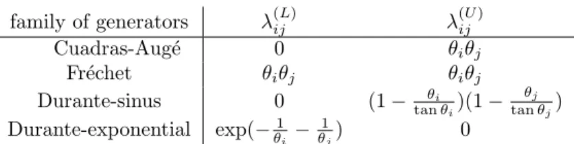
The four above examples allow to get all possible types of tail dependencies, as shown in Table 1. The Cuadras-Aug´e and Durante-sinus families allow for upper but no lower tail dependence, the Durante-exponential family allows for lower but no upper tail dependence, and the Fr´echet family allows for both. In the Fr´echet case, furthermore, the lower and upper tail dependence coefficients are equal: this is called tail symmetry, a property of elliptical copulas.
2.4
Extreme-value attractors associated to FDG copulas
Extreme-value copulas are theoretically well-grounded copulas to perform a sta-tistical analysis of extreme values such as maxima of random samples. Recall that a copulaC#is an extreme-value copula if there exists a copula ˜Csuch that
C#(u1, . . . , ud) = lim n↑∞Ce n(u1/n 1 , . . . , u 1/n d ), (u1, . . . , ud)∈[0,1]d, (10)
family of generators λ(ijL) λ(ijU) Cuadras-Aug´e 0 θiθj Fr´echet θiθj θiθj Durante-sinus 0 (1− θi tanθi)(1− θj tanθj) Durante-exponential exp(−1 θi − 1 θj) 0
Table 1: Lower λ(ijL) and upper λ(ijU) tail dependence coefficients for the four families presented in Section 2.3.
see, e.g. [21]. The extreme-value copula C# is called the attractor of Ce and e
C is said to belong to the domain of attraction of C#. The class of
extreme-value copulas corresponds exactly to the class of max-stable copulas, that is, the copulasC#such that
C#n(u11/n, . . . , ud1/n) =C#(u1, . . . , ud), n≥1,(u1, . . . , ud)∈[0,1]d. The upper tail dependence coefficient of a (bivariate) extreme-value copula C#
has the particular form
λ(U)= 2 + logC#(e−1, e−1). (11)
This coefficient is a natural dependence coefficient for extreme-value copulas because of the following representation on the diagonal of the unit square:
C#(u, u) =u2−λ, (12)
whereλ:=λ(U). Ifλ= 0 thenC
#(u, u) = Π(u, u) =u2, where Π stands for the
independence copula. Ifλ= 1 thenC#(u, u) =M(u, u) = min(u, u) =u, where
M stands for the Fr´echet-Hoeffding upper bound for copulas, that is, the case of perfect dependence. In the case of extreme-value copulas, this interpolation between Π and M allows to interpret λ as a coefficient that measures general dependence, not only dependence in the tails. In order to emphasize this in-terpretation, λwill be referred to as the extremal dependence coefficient of an extreme-value copula. See [6] for more about extreme-value statistics, and, see, e.g. [21] for an account about extreme-value copulas.
In the case of FDG copulas, the limit (10) can be calculated. This leads to a new family of extreme-value copulas, referred to as the EV-FDG family. The bivariate margins C#,ij of this new family are Cuadras-Aug´e copulas. These results are specified in Theorem 2 and Proposition 3 below.
Theorem 2. Assume that the generators fi of the FDG copula are twice
con-tinuously differentiable on [0,1]. Then, the attractor C# of the FDG copula
exists and is given by
C#(u1, . . . , ud) = d Y i=1 uχi (i), (13) where χi= i−1 Y j=1 (1−λ(j)) λ(i)+ 1−λ(i),
with the convention thatQ0
j=1(1−λ(j)) = 1and whereλi= 1−fi0(1). As in(3),
u(i)=uσ(i) andf(0i)(1) =f 0
σ(i)(1)where σis the permutation of (1, . . . , d)such
that u(1) ≤ · · · ≤u(d).
Proposition 3. Let C#,ij be a bivariate margin of the EV-FDG copula (13).
Then C#,ij is a Cuadras-Aug´e copula with parameter (and therefore extremal
dependence coefficient)λiλj. In other words,
C#,ij(ui, uj) = min(ui, uj) max(ui, uj)1−λiλj. (14)
Remark 2. In view of Table 1, the FDG copulas with Cuadras-Aug´e and Fr´echet generators both lead to the same EV-FDG copula.
Multivariate generalizations of the bivariate Cuadras-Aug´e copula were already proposed in the literature [14, 29], but they are less flexible than EV-FDG. Indeed, let us consider the following exchangeable copula proposed in [29],
A(u1, . . . , ud) =u(1) d Y i=2 uai (i),
where (a1= 1, a2, a3, . . . , ad) is ad-monotone sequence of real numbers, that is,
a sequence which satisfiesOj−1ak ≥0, k= 1, . . . , d, j= 1, . . . , d−k+ 1 where
Ojak =P j i=0(−1) i j i
ak+i, j, k≥1 andO0ak=ak. In particular, the bivariate margins are Cuadras-Aug´e copulas
Aij(ui, uj) = min(ui, uj) max(ui, uj)a2
with the same parameter 1−a2. This means that all of them exhibit the same
statistical behavior. For instance, all the upper tail dependence coefficients are equal and are given by 1−a2. This is far too restrictive for most applications.
Then let us consider the generalization proposed in [14],
B(u1, . . . , ud) = d Y i=1 u1− Pd j=1,j6=iλij i Y i<j min(ui, uj)λij, whereλij ∈[0,1], λij =λji and X j=1,...,d;j6=i λij≤1, i= 1, . . . , d. (15)
The bivariate marginsBij are Cuadras-Aug´e copulas
Bij(ui, uj) = min(ui, uj) max(ui, uj)1−λij
with parametersλij. Unlike the copula A, the tail dependence coefficients can take distinct values. Unfortunately, the constraints (15) are quite restrictive, as it was already stressed by the original authors in [14]. The EV-FDG class achieves greater flexibility than these competitors. In particular, one can obtain different bivariate marginal distributions withnoconditions on the parameters.
3
Parametric inference
Let (X1, . . . , Xd) be a random vector following a distributionF with continuous
marginsF1, . . . , Fd. Suppose that its copula,C, is a FDG copula defined by (3).
Denote by (X1(k), . . . , Xd(k)),k= 1, . . . , nindependent and identically distributed observations obtained from F. Suppose that all the generatorsfi of the FDG copula belong to the same parametric family {fθ, θ ∈ Θ⊂ R}, that is, there exists θ0 = (θ01, . . . , θ0d) ∈ Θd such that fθ0i = fi. The generators fi are
regarded as functions defined over the product space [0,1]×Θ and we write
fi(t) = f(t, θi) for all t in [0,1]. The nonparametric inference problem has turned into a parametric one where the parameter vector θ0 ∈ Θd has to be
estimated.
In order to estimate the parameters of the FDG and EV-FDG copulas, a least-squares estimator based on dependence coefficients is adopted. This esti-mation strategy was considered in various articles, see e.g. [14, 18–20, 24, 30, 33]. Its construction is recalled below. Let us choose a type of dependence coeffi-cient (Spearman’s rho, Kendall’s tau, tail dependence coefficoeffi-cient, etc) and let us denote by r(θi, θj) the chosen dependence coefficient between the variables
Xi and Xj. Suppose that the map r is continuous and symmetric in its argu-ments. Let p = d(d−1)/2 be the number of variable pairs (Xi, Xj), i < j. Denote by r be the p-variate map defined on Θd such that r(θ1, . . . , θd) =
(r(θ1, θ2), . . . , r(θd−1, θd)). The least-squares estimator based on dependence
coefficients is defined as
ˆ
θ= arg min
θ∈Θd
kˆr−r(θ)k2, (16)
where the quantityˆr= (ˆr1,2, . . . ,rˆd−1,d) is an empirical estimator ofr(θ0). To
be more specific,r(θi, θj) may be the Spearman’s rho (4) of (Xi, Xj) and
ˆ ri,j = Pn k=1 ˆ Ui(k)−Uˆi Uˆ (k) j −Uˆj Pn k=1 ˆ Ui(k)−Uˆi 2 Pn k=1 ˆ Uj(k)−Uˆj 21/2 , (17) where ˆUi=Pnk=1U (k) i /nand ˆU (k) i = Pn l=11(X (l) i ≤X (k) i )/(n+ 1). In the case wherer(θi, θj) is the Kendall’s tau (4) of (Xi, Xj), then
ˆ ri,j= n 2 −1 X k<l sign(Xi(k)−Xi(l))(Xj(k)−Xj(l)), (18)
where sign(x) = 1 if x > 0, −1 if x < 0 and 0 if x = 0. Equation (12) suggests that the extremal dependence coefficient can also be used to estimate the parameters of an extreme-value copula. If the marginsFiare known, various empirical estimators of the extremal dependence exist. For instance, assuming that Cis an extreme-value copulas, [15] introduced
ˆ ri,j= 3− 1 1−Pn k=1max(U (k) i , U (k) j )/n , (19) whereUi(k)=Fi(Xi(k)).
In the context of non-absolutely continuous copulas with respect to the Lebesgue measure – as FDG copulas –, asymptotic properties of (16) were derived in [30], see the proposition below.
Proposition 4. Suppose that the following assumptions hold. (A1) √n(ˆr−r(θ0))
d
→ N(0,Σ) as n → ∞ for some symmetric and positive definite matrixΣ.
(A2) The mapris a twice continuously differentiable homeomorphism fromΘd
to its imager(Θd).
(A3) The Jacobian matrixJof the map ratθ0 is of full rank.
Then, as n → ∞, the estimator θˆdefined in (16) is unique with probability tending to one, consistent forθ0, and asymptotically normal
√ n(θˆ−θ0) d →N(0,Ξ), whereΞ= JTJ−1 JTΣJ JTJ−1 .
There exist various situations where (A1) holds, as, for instance, in the context of Spearman’s rho (estimator (17)) and Kendall’s tau dependence coefficients (estimator (18)), see [22] for a proof. In the context of extreme-value copulas with known margins, (A1) also holds for the extremal dependence coefficient (estimator (19)), see [30] for a proof.
The remaining of this section is devoted to show that, for certain (EV-)FDG copulas, we are able to show that the assumptions of Proposition 4 hold.
Lemma 1. (i) Define the univariate function rθj(θi) := r(θi, θj) and
as-sume that it is a twice continuously differentiable homeomorphism. Let
r1,2, . . . , rd−1,d be p elements of r(Θd). Define si,j(θ) := r−1θ (ri,j) for
θ∈Θ. Then, the function s1,3◦s1,2◦s2,3 has at least one fix point, that
is, the equation
s1,3◦s1,2◦s2,3(θ) =θ, θ∈Θ (20)
has at least one solution.
(ii) If, moreover, the functions1,3◦s1,2◦s2,3has exactly one fix point, that is,
equation (20) has exactly one solution, then assumptions (A2) and (A3) of Proposition 4 hold.
Remarking that the extremal dependence coefficients of the EV-FDG bivariate margins writeλi,j(θ) =λ(θi)λ(θj), withλ(θ) = 1−∂f∂t(t,θ)
t=1,θ∈Θ, allows to
apply Lemma 1 and therefore to satisfy the assumptions of Proposition 4. The next theorem thus provides some situations where the least-squares estimator is unique with probability tending to one, consistent, and asymptotically Gaussian.
Theorem 3. (i) Assume that(X1, . . . , Xd)has EV-FDG (13)as copula and
let r(θi, θj) be the extremal dependence coefficient of (Xi, Xj). Consider
one of the following cases:
• The generators are Cuadras-Aug´e (4)andΘ = (0,1).
• The generators are Fr´echet (5) andΘ = (0,1).
Then, assumptions (A1), (A2) and (A3) of Proposition 4 hold withˆrbeing as in (19).
(ii) Assume that the copula of(X1, . . . , Xd)belongs to the class of FDG copulas
given in Example 2 and suppose thatr(θi, θj)is Spearman’s rho coefficient
of (Xi, Xj) andˆris as in (17). Then, assumptions (A1), (A2) and (A3)
of Proposition 4 hold.
4
Applications to simulated and real datasets
The modeling of data with (EV-)FDG copulas is illustrated through numerical experiments in Section 4.1 and a real dataset application in Section 4.2. In the numerical experiments, we first provide empirical evidence that the proposed FDG copulas are well suited for high-dimensional applications. In the real dataset application, critical levels of potentially dangerous hydrological events are estimated. Throughout this section, the four copulas of Example 1–4, are respectively referred to as FDG-CA, FDG-F, FDG-sinus, and FDG-exponential. The minimization of the loss function (16) was carried out with standard gradient descent algorithms whose implementations can be found in the
func-tion optim from the R software [34]. In principle, several runs with different
starting points should be tested to ensure that the global minimizer is reached. Also, formal statistical procedures can be performed to test wether the given minimizer is indeed the global minimizer; see [8, 9, 35]. We found that a single run was enough to find what appeared to be the global optimum. Thus, the loss functions one encounters when dealing with FDG copulas seem to be easy to minimize in practice. All the experiments were conducted using theFDG pack-age that we developed and which is freely available on the CRAN archive at
http://cran.r-project.org/web/packages/FDG.
4.1
Numerical experiments
Our first goal is to investigate the numerical behavior of the estimation of FDG copulas as the sample size varies from n = 10 to n = 500 with fixed d = 9 (as in the real dataset application). To this aim, 200 datasets are simulated from each of the copulas FDG-CA, FDG-F, FDG-sinus, and FDG-exponential. The coordinates of the parameter vector were chosen to be regularly spaced within [0.3,0.9],[0.3,0.9],[1,1.55] and [3,20] for FDG-CA, FDG-F, FDG-sinus, and FDG-exponential respectively. For each replication and each model, the samples are simulated from the copula using the principle described in Sec-tion 2. The model parameters are estimated by the least squares estimator (16) combined with Spearman’s rho dependence coefficient as in (17). The accuracy of the method is assessed using the mean absolute error and the relative mean absolute error, respectively defined as
MAEr= 1
p
X
i<j
|ri,j−r(ˆθi,θˆj)| and RMAE = 1 d d X i=1 |θˆi−θ0i| θ0i ,
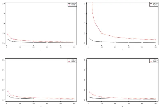
computed and averaged over the replications. It appears on Figure 1 that the MAEρs are very stable whatever the sample size. CA, F and FDG-sinus models also provide good results in terms of RMAE provided that the
sample size is larger thann= 30. At the opposite, it seems that the estimation of FDG-exponential model requires large sample sizes.
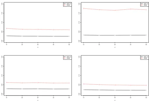
The second experiment examines the scalability of the FDG copulas when the dimension increases from d = 10 to d = 50 for a fixed sample size n = 500. Similarly to the previous experiment, the coordinates of the parameter vector were chosen to be regularly spaced within [0.3,0.9],[0.3,0.9],[1,1.55] and [3,20] for FDG-CA, FDG-F, FDG-sinus, and FDG-exponential respectively. It appears on Figure 2 that the MAEρs and RMAEs are very stable whatever the dimension. The inference for these models seems not to be sensitive to the dimension. FDG-exponential has a larger RMAE, but it is still below 17%, and its MAEρ is as good as that of the other models.
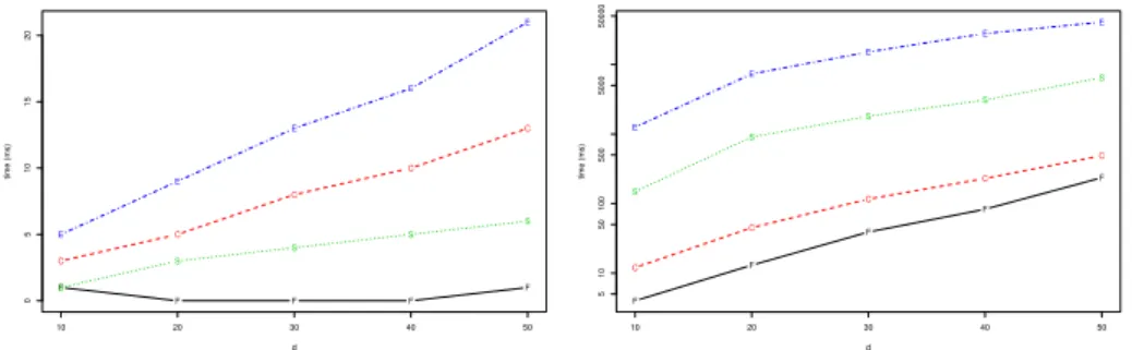
Figure 3 displays the associated computed times for one sample on a 8 GiB memory and 3.20 GHz processor computer. The simulation time increases lin-early with the dimension whereas the estimation time increases exponentially. Simulating all the models even in high dimension is instantaneous because of the conditional independence property seen in (1). Less than two minutes are necessary to fit all the models. In particular, simulating or fitting FDG-F is instantaneous. The computational costs for performing the inference of FDG-exponential and FDG-sinus are larger because their dependence coefficient ex-pressions, given in Example 3 and 4, involve integrals which have to be computed numerically. To summarize, FDG copulas seem to scale up well.
1 1 1 1 1 1 1 1 0 100 200 300 400 500 0.0 0.5 1.0 1.5 2.0 n 2 2 2 2 2 2 2 2 1 2 MAE rho RMAE 1 1 1 1 1 1 1 1 0 100 200 300 400 500 0.0 0.5 1.0 1.5 2.0 n 2 2 2 2 2 2 2 1 2 MAE rho RMAE 1 1 1 1 1 1 1 1 0 100 200 300 400 500 0.0 0.5 1.0 1.5 2.0 n 2 2 2 2 2 2 2 2 1 2 MAE rho RMAE 1 1 1 1 1 1 1 1 0 100 200 300 400 500 0.0 0.5 1.0 1.5 2.0 n 2 2 2 2 2 2 2 2 1 2 MAE rho RMAE
Figure 1: Fitting errors as a function of the sample size n for a dimension
d= 9. Continuous line (1): MAEρ, Dashed line (2): RMAE. Four copulas were tested (FDG-CA: upper left, FDG-exponential: upper right, FDG-F: lower left, FDG-Sinus: lower right).
1 1 1 1 1 10 20 30 40 50 0.00 0.05 0.10 0.15 0.20 d 2 2 2 2 2 1 2 MAE rho RMAE 1 1 1 1 1 10 20 30 40 50 0.00 0.05 0.10 0.15 0.20 d 2 2 2 2 2 1 2 MAE rho RMAE 1 1 1 1 1 10 20 30 40 50 0.00 0.05 0.10 0.15 0.20 d 2 2 2 2 2 1 2 MAE rho RMAE 1 1 1 1 1 10 20 30 40 50 0.00 0.05 0.10 0.15 0.20 d 2 2 2 2 2 1 2 MAE rho RMAE
Figure 2: Fitting errors as a function of the dimension d for a sample size
n = 500. Continous line (1): MAEρ, Dashed line (2): RMAE. Four copulas were tested (FDG-CA: upper left, FDG-exponential: upper right, FDG-F: lower left, FDG-Sinus: lower right).
4.2
Application to a hydrological dataset
4.2.1 Data and Context
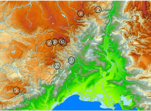
The dataset consists of n = 32 observations (X1(k), . . . , Xd(k)), k = 1, . . . , n, of annual maxima river flow rates located at d= 9 sites across south-east France between 1969 and 2007 (some records are missing). Let us denote byF the dis-tribution with continuous marginsF1, . . . , Fdof the random vector (X1, . . . , Xd)
whose realizations provide the observed dataset. The location of the sites are shown in Figure 4. The number of variable pairs isp= 36. Due to the hetero-geneous dispersion of the sites, the span of positive dependence is almost maxi-mum; for instance, Spearman’s rho dependence coefficients range from about 0 to 0.9.
In hydrology, it is of interest to get information about the statistical distri-bution of a potentially dangerous event, such as{F1(X1)> q, . . . , Fd(Xd)> q}, or, equivalently, {min(F1(X1), . . . , Fd(Xd)) > q}, where q is the critical level associated to that event. Thereturn period T is defined as
T = 1
1−M(q), whereM(q) =P(min(F1(X1), . . . , Fd(Xd))≤q). (21) For instance, a return period ofT = 30 years and a critical level ofq= 0.7 means that each Xi exceeds its quantile of order 70% once every 30 years in average. A common question in the study of extreme events is the following. Given a return period T, how dangerous is the corresponding event? In other words,
F F F F F 10 20 30 40 50 0 5 10 15 20 d time (ms) C C C C C S S S S S E E E E E F F F F F 10 20 30 40 50 5 10 50 100 500 5000 50000 d time (ms) C C C C C S S S S S E E E E E
Figure 3: Computation times (in milliseconds) as a function of the dimension
d for a sample of size n = 500. Left panel: Simulation of the copula, right panel: Estimation of the parameters. Four copulas were tested (C: FDG-CA, F: FDG-F, S: FDG-Sinus, E: FDG-exponential).
what is the associated critical levelq? The answer is obtained by inverting (21)
q=M−1 1− 1 T . (22)
Thus, the answer q is the quantile of order 1−1/T of the distribution M. This quantile can be estimated empirically from the data and parametrically by fitting a model to the data.
Potentially dangerous events happen with the co-occurrence of extremely high flow rates at several locations. Thus, it is clear that the models to de-scribe this dataset should be upper tail dependent. Hence, good candidates are the copulas of Example 1–3, referred to as FDG-CA, FDG-F, and FDG-sinus respectively, and all the extreme-value copulas. However, as it was shown in Remark 1, Spearman’s rho of FDG-sinus cannot take values greater than 0.37. Hence, this copula is removed from the candidate models. So the considered models are FDG-CA, FDG-F, and their extreme-value attractor EV-FDG-CAF given in (13) (recall that FDG-CA and FDG-F lead to the same extreme-value copula). Two other popular copula models, the Gumbel and Student copulas, are also fitted to the data. The Gumbel copula is famous among hydrologists [36] and the Student copula is well known in risk management [31]. They serve as a benchmark for our models. A factor structure is assumed for the Student copula, that is, its (i, j)-th element (i6=j) of its correlation matrix writesθiθj, where θ1, . . . , θd belong to [−1,1]. Recall that a Gumbel copula is an extreme-value copula. More details about the Gumbel and the Student copula can be found respectively in, e.g., [23, 32] and [10].
4.2.2 Method and Results
A practically convenient approach dictated the estimation of the copula param-eters. For each copula model, the dependence coefficients with the simplest mathematical forms were chosen to build the loss function (16). In other words, the parameters of FDG-F, FDG-CA and EV-FDG-CAF were estimated with Spearman’s rho as in (17). The parameters of the Gumbel and Student copulas were estimated with Kendall’s tau as in (18). Finally, the degree of freedom of
Figure 4: Location of the 9 sites for the flow rate dataset. The sea in dark blue at the bottom (south) is the Mediterranean sea. The rivers are shown in light blue. The river flowing from north to south in the green area is the Rhˆone. Green indicates low altitude, and orange high altitude. The map of this figure was drawn with G´eoportail (www.geoportail.gouv.fr).
the Student copula was estimated by maximizing its likelihood but with all the parameters of the correlation matrix held fixed. This approach improves the speed, tractability, and chances of success of the minimization procedure.
The fit of the tested copulas was assessed by comparing the pairwise depen-dence coefficients and the critical levels.
Pairwise dependence coefficients. The mean absolute error (MAE), de-fined as M AEr= 1 p X i<j rˆi,j−r(ˆθi,θˆj)
was computed for Spearman’s rho (MAEρ) and Kendall’s tau (MAEτ) depen-dence coefficients. They are reported in Table 2. The Gumbel copula has the largest errors (more than 0.17) and does not seem to fit the data well. This was expected, because this model has only one parameter to account for a d = 9 dimensional phenomenon. All the remaining errors are smaller. Thus, according to these criteria, the Gumbel copula is not appropriate.
Critical levels. The critical levels obtained from the empirical data and the models were calculated by making use of (22). In statistical terms, this amounts to compare the quantiles of the distribution M under the empirical data and
FDG-F FDG-CA EV-FDG-CAF Gumbel Student MAEρ 0.12 0.12 0.12 0.22 0.12 MAEτ 0.12 0.11 0.11 0.17 0.10
Table 2: Mean absolute errors for Spearman’s rho (MAEρ) and Kendall’s tau (MAEτ) dependence coefficients of the models.
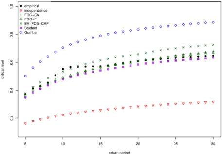
under the different models. The results are presented in Figure 5, where the independence copulaC(u1, . . . , ud) =u1. . . udwas added to emphasize the need for a joint model on such a dataset. The Gumbel model is confirmed to perform poorly. FDG-F, FDG-CA and EV-FDG-CAF seem to fit the data quite well. In particular, FDG-F and FDG-CA are as close as the Student copula to the empirical curve. 5 10 15 20 25 30 0.2 0.4 0.6 0.8 1.0 return period cr itical le vel empirical independence FDG−CA FDG−F EV−FDG−CAF Student Gumbel
Figure 5: Critical levelqas a function of the return periodT. “empirical” stands for the empirical critical levels, and “independence” for the independence copula
C(u1, . . . , ud) =Q
d i=1ui.
With such a small sample sizen= 32, one must be extremely careful when looking at empirical data, because one is likely to observe a large deviation from the true underlying statistical distribution. In view of this remark, one should select a statistical model based not only on empirical data, but also on the model properties. The class of FDG copulas is very interesting in this respect. Indeed, the practitioner has with this class three models that fit well the data and with different features: F is upper, lower, and symmetric tail dependent, FDG-CA is upper tail dependent but no lower tail dependent, and EV-FDG-FDG-CAF is an extreme-value copula. The user is then free to choose the model that most suits his expert knowledge about the underlying phenomenon at play. The test
of extreme-value dependence [25] gave a p-value of 0.21, which means that one does not reject extreme-value copulas at the 5% level. Of course, as before, one must be extremely careful when looking at the p-value because of the small data sample size. Finally, goodness-of-fit tests for a given parametric family can be found in [26].
5
Discussion
In this article, we have constructed a new class of copulas by combining one-factor copulas, that is, a conditional independent property, together with a class of bivariate copulas called the Durante class of bivariate copulas. This combi-nation led to many advantageous properties. The copulas within the proposed class, referred to as FDG copulas, are tractable, flexible, and cover all types of tail dependencies. The theoretically well grounded least-squares inference estimator is particularly well suited for FDG copulas because their dependence coefficients are easy to compute, if not in closed form. This allows to perform fast and reliable inference in the parametric case. We have demonstrated, fur-thermore, that FDG copulas work well in practice and are able to model both high-dimensional and real datasets. Finally, we have derived the extreme-value copulas (EV-FDG) associated to FDG copulas, yielding a new extreme-value copula, which can be viewed as a generalisation of the well-known Cuadras-Aug´e copula. This copula benefits from almost all the many advantageous properties of FDG copulas, and therefore opens the door for statistical analyses of extreme data in high dimension.
One may argue that a model with a singular component, as a FDG copula, is not natural nor realistic to model hydrological data. While this may be true in the bivariate case, this argument becomes weaker when the dimension increases. Indeed, in high-dimensional applications, the focus is less on the distribution itself than on a feature of interest of the data, such as, for instance, the critical levels defined in (22). If so-called “unrealistic” models are able to better estimate these features than “realistic” models – compare the fit of the Gumbel copula to the fit of FDG copulas in Section 4.2 – then one should consider using them. This work raises several research questions. First, how to estimate the gen-erators nonparametrically? The generator of a bivariate Durante copula was estimated nonparametrically in [12], but the matter is more complicated in our case because this bivariate relationship occurs between the variable of interest and the unobserved latent factor. Second, one may add more factors when building an FDG copula. Nonetheless, the model might not be as tractable as it is and therefore it may be less appealing in practice. Finally, FDG copulas possess the conditional independence property, but the extreme-value EV-FDG copulas were not shown to do so. If this property held, this would be of great interest for the simulation of datasets from this model.
Acknowledgments. The authors thank “Banque HYDRO du Minist`ere de l’ ´Ecologie, du D´eveloppement durable et de l’ ´Energie” for providing the data and Benjamin Renard for fruitful discussions about statistical issues in hydrological science. They also thank two anonymous referees and the associate editor for helpful suggestions and comments.
A
Appendix
Proof of Theorem 1 Let Cj|0(·|u0) be the conditional distribution of Uj givenU0=u0. TheUj’s are conditionally independent givenU0, hence,
C(u) = Z 1 0 d Y j=1 Cj|0(uj|u0)du0 (23) = Z 1 0 d Y j=1 ∂C0j(u0, uj) ∂u0 du0 = Z 1 0 d Y j=1 ∂C0(j)(u0, u(j)) ∂u0 du0 = Z u(1) 0 d Y j=1 ∂C0(j)(u0, u(j)) ∂u0 du0 + d X k=2 Z u(k) u(k−1) k−1 Y j=1 ∂C0(j)(u0, u(j)) ∂u0 d Y j=k ∂C0(j)(u0, u(j)) ∂u0 + Z 1 u(d) d Y j=1 ∂C0(j)(u0, u(j)) ∂u0 du0. Since ∂C0j(u0, uj) ∂u0 = fj(uj) ifu0< uj ujfj0(u0) ifu0> uj, equation (23) yields C(u) =u(1) d Y j=1 fj(uj) + d X k=2 d Y j=k f(j)(u(j)) Z u(k) u(k−1) k−1 Y j=1 u(j)f(0j)(u0)du0 + d Y j=1 uj Z 1 u(d) fj0(u0)du0.
Putting u(1) in factor and noting that
Ru(2)
u(1) f 0
(1)(x)dx =f(1)(u(2))−f(1)(u(1))
finishes the proof.
Proof of Proposition 1 It suffices to set all uk equal to one butui and uj in the formula (3).
Proof of Proposition 2 It suffices to apply the formulas (4) with fij given in Proposition 1. To compute the Spearman’s rho, note that
Z 1 0 x2fij(x)dx= Z 1 0 x2fi(x)fj(x)dx+ Z 1 0 x3 Z 1 x fi0(z)fj0(z)dzdx.
An integration by parts yieldsR1
0 x 3R1 x f 0 i(z)fj0(z)dzdx= (1/4) R1 0 x 4f0 i(x)fj0(x)dx and the result follows.
Proof of Theorem 2 Fix (u1, . . . , ud)∈[0,1]d and let n≥1 be an integer. Let us introduce αn:=u 1/n (1) Qd j=1 fj(u1j/n) u1j/n , βn := Z 1 u1(d/n) d Y j=1 fj0(u0)du0, γn:=Qdj=k f(j)(u 1/n (j)) u1(j/n) , δn,k := Z u1(k/n) u1(k/n−1) k−1 Y j=1 f(0j)(u0)du0, and define An :=αn+βn+ d X k=2 γn,kδn,k.
Our goal is to derive asymptotic equivalent sequences forαn, βnγn andδn. Let
∼ denote the equivalent symbol at infinity (i.e., an ∼ bn means an/bn → 1 as n → ∞). By using the well known formulas ex ∼ 1 +x (when x → 0), logx∼x−1 (whenx→1) andfj(x)∼1 + (x−1)fj0(1) (whenx→1), we get
αn∼ 1 + 1 nlogu(1) 1− 1 nlog(u1. . . ud) 1 + 1 n d X j=1 logu(j)f(0j)(1) and γn,k∼ 1− 1 n d X j=k logu(j) 1 + 1 n d X j=k logu(j)f(0j)(1) .
For βn the equivalence is obtained as follows. Let F(x) be a primitive of
Qd
j=1f 0
j(x). It follows thatβn=F(1)−F(u
1/n
(d)). A Taylor expansion yields
F(u1(d/n)) =F(1) + (u1(d/n) −1)F0(1) + (u1(d/n) −1)2 2 F 00(xn) wherexn is betweenu 1/n (d) and 1. SinceF 00is assumed to be continuous on [0,1],
it is uniformly bounded on this set and therefore (u1(d/n) −1)2F00(xn)/2 =o(1/n) where o(1/n) is a quantity such that no(1/n) → 0 as n → ∞. Hence, since
u1(d/n) = exp(log(u(d))/n)∼1 + log(u(d))/n, we have asn→ ∞
F(1)−F(u1(d/n))∼ −1
nlog(u(d))F
0(1).
The same arguments apply to get
βn ∼ − 1 nlogu(d) d Y j=1 fj0(1) δn,k ∼ 1 nlog u (k) u(k−1) k−1 Y j=1 f(0j)(1).
The quantity An is a polynomial with respect to n−1 of order at most three. In (24), the coefficients of order 0, 2, and 3 vanish at infinity. Only remain the terms of order 1, hence,
lim n↑∞n(An−1) = logu(1)−log(u1. . . ud) + d X j=1 logu(j)f(0j)(1) (24) −logu(d) d Y j=1 f(0j)(1) + d X k=2 k−1 Y j=1 f(0j)(1) log u (k) u(k−1) .
From Abel’s identity for two sequences (ai) and (bi) of real numbers, that is, d−1 X i=1 ai(bi+1−bi) = d−1 X i=1 bi(ai−1−ai) +ad−1bd−a1b1 it follows lim n↑∞n(An−1) = d X k=1 k−1 Y j=1 f(0j)(1) (1−f(0k)(1)) +f(0k)(1)−1 | {z } =:χk logu(k),
with the convention thatQ0
j=1f(0j)(1) = 1. Then (3) entails that
Cn(u11/n, . . . , ud1/n) =u1. . . udexp [nlogAn] =u1. . . udexp [n(An−1)(1 +o(1))] → d Y i=k uχk (k) as n→ ∞.
Proof of Lemma 1 (i) Since thep-uple (r1,2, . . . , rd−1,d) belongs to the image
spacer(Θd), the system
r(θ1, θ2) = r1,2 .. . ... r(θd−1, θd) = rd−1,d
has at least one solution. In particular, there exists (θ1, θ2, θ3) in Θ3 such that
r(θ1, θ2) = r1,2 r(θ1, θ3) = r1,3 r(θ2, θ3) = r2,3. (25)
The system (25) rewrites
rθ2(θ1) = r1,2 rθ3(θ1) = r1,3 rθ3(θ2) = r2,3,
or equivalently, θ1 = s1,2(θ2) θ1 = s1,3(θ3) θ2 = s2,3(θ3). This yields s1,3(θ3) =s1,2◦s2,3(θ3). (26)
Let us note that s1,3 is involutive at θ3, that is, s1,3◦s1,3(θ3) = θ3. Indeed,
r(θ1, θ3) = rθ3(θ1) = r1,3 is equivalent to θ1 = r −1
θ3(r1,3) = s1,3(θ3). This
implies r(s1,3(θ3), θ3) =r1,3, and, composing by r−1s1,3(θ3) in both sides, we get
r−1s
1,3(θ3)(r1,3) = s1,3(s1,3(θ3)) = θ3. Therefore, one can compose both sides
of (26) bys1,3 to get
θ3=s1,3◦s1,2◦s2,3(θ3).
Hence (20) has at least one solution.
(ii) If (20) admits exactly one solution θ3, then θ2 andθ1 are also unique.
Furthermore, for all j≥3,
θj+1=sj,j+1(θj)
which concludes the proof that assumption (A2) holds. It is now shown that assumption (A3) holds as well. Define∂1r, respectively,∂2r, the derivative ofr
with respect to the first, respectively, second, variable ofr. Hence for allθi and
θj in Θ, the quantities ∂1r(θi, θj) andrθj(θi) only differ in the notation. The
first step in the proof is to consider the case d= 3. The Jacobian matrix ofr
atθ0is given by J= ∂1r(θ01, θ02) ∂2r(θ01, θ02) 0 ∂1r(θ01, θ03) 0 ∂2r(θ01, θ03) 0 ∂1r(θ02, θ03) ∂2r(θ02, θ03) .
To show that Jhas full rank, we show that its determinant
∂1r(θ01, θ02)∂2r(θ01, θ03)∂1r(θ02, θ03) +∂2r(θ02, θ03)∂1r(θ01, θ03)∂2r(θ01, θ02)
is nonzero. Indeed, note that for allθ in Θ, the maprθ: Θ→rθ(Θ) is a twice continuously differentiable homeomorphism. Furthermore, by assumption, the true parameter vector θ0 lies in the interior of Θ that is open. Finally, by
symmetry, for all i < j,
∂r1(θ0i, θ0j)>0 (respectively∂r1(θ0i, θ0j)<0)
is equivalent to
∂r2(θ0j, θ0i)>0 (respectively∂r2(θ0j, θ0i)<0).
For the general case, we proceed by mathematical induction. When the dimension is d, writeJ(θ) = J(d)(θ) to emphasize the dependence on the
di-mension. Notice that it was already shown above that J(3)(θ) has full rank.
Now suppose that the kernel of J(d−1)(θ) is null when the dimension isd−1.
LetA=J(d)(θ). Each row ofAwrites
where ∂1r(θi, θj) is at the i-th position and ∂2r(θi, θj) at the j-th position. There ared−1 rows ofAwhich depend onθdandp−d+ 1 which do not (recall
p=d(d−1)/2 is the number of pairs). Since the kernel of a matrix is invariant by permutation, we can without loss of generality put all the rows which do not depend onθd on the top. More precisely, decomposeAas
A=
A11 A12
A21 A22
such thatA11is a (p−d+ 1)×(d−1) matrix containing all the rows which do
not depend onθdandA12andA22 are (p−d+ 1)×1 and (d−1)×1 matrices
respectively. Note that A12is the null vector of sizep−d+ 1×1. Letx∈Rd,
x= (xT
1, x2)T wherex1 ∈Rd−1, x2 ∈R. It follows that Ax=0is equivalent to
A11x1+A12x2=0
A21x1+A22x2= 0.
But A12 =0 and sinceA11 = J(d−1)(θ) whose kernel is null, x1 =0. Then
A22x2= 0 and the assumptions implyx2= 0, which concludes the proof.
Proof of Theorem 3 To prove (i), it suffices to apply Lemma 1. Since
r(θi, θj) denotes the extremal dependence coefficient of the E copula bivariate marginal C#,ij defined in (14), we have
r(θi, θj) =λ(θi)λ(θj), whereλ(θ) := 1− ∂f(t, θ) ∂t t=1. (27)
In the Cuadras-Aug´e and the Fr´echet cases, (27) is given by λ(θ) = θ, and in the sinus case, λ(θ) = 1−θ/tan(θ). In all these situations, it is easy to see that the map rθj(·) is a twice continuously differentiable homeomorphism.
Therefore, Lemma 1 (i) applies. To apply the second part of Lemma 1, note that equation (20) translates into
λ(θ)2=r1,3r2,3
r1,2
.
Since it has a unique solution, Lemma 1 (ii) applies, and the result is proved. (ii) The proof is straightforward because under the assumptions of (ii),
r(θi, θj) = θiθj. But this is the precise form of r(θi, θj) in (i); hence, one can also apply Lemma 1.
References
[1] K. Aas, C. Czado, A. Frigessi, and H. Bakken. Pair-copula constructions of multiple dependence. Insurance: Mathematics and Economics, 44(2):182– 198, 2009.
[2] E. F. Acar, C. Genest, and J. Neˇslehov´a. Beyond simplified pair-copula constructions. Journal of Multivariate Analysis, 110:74–90, 2012.
[3] C. Amblard and S. Girard. A new extension of bivariate FGM copulas.
[4] T. Bedford and R.M. Cooke. Probability density decomposition for condi-tionally dependent random variables modeled by vines. Annals of Mathe-matics and Artificial intelligence, 32(1-4):245–268, 2001.
[5] T. Bedford and R.M. Cooke. Vines–a new graphical model for dependent random variables. The Annals of Statistics, 30(4):1031–1068, 2002. [6] S. Coles.An introduction to statistical modeling of extreme values. Springer,
2001.
[7] C.M. Cuadras and J. Aug´e. A continuous general multivariate distribution and its properties. Communications in Statistics - Theory and Methods, 10(4):339–353, 1981.
[8] M. De Carvalho. Confidence intervals for the minimum of a function using extreme value statistics. International Journal of Mathematical Modelling and Numerical Optimisation, 2(3):288–296, 2011.
[9] M. de Carvalho. A generalization of the solis–wets method. Journal of Statistical Planning and Inference, 142(3):633–644, 2012.
[10] S. Demarta and A. J. McNeil. The t copula and related copulas. Interna-tional statistical review, 73(1):111–129, 2005.
[11] F. Durante. A new class of symmetric bivariate copulas. Nonparametric Statistics, 18(7-8):499–510, 2006.
[12] F. Durante and O. Okhrin. Estimation procedures for exchangeable mar-shall copulas with hydrological application. Stochastic Environmental Re-search and Risk Assessment, published online, 2014.
[13] F. Durante, J.J. Quesada-Molina, and M. ´Ubeda Flores. On a family of multivariate copulas for aggregation processes. Information Sciences, 177(24):5715–5724, 2007.
[14] F. Durante and G. Salvadori. On the construction of multivariate extreme value models via copulas. Environmetrics, 21(2):143–161, 2010.
[15] M. Ferreira. Nonparametric estimation of the tail-dependence coefficient.
REVSTAT–Statistical Journal, 11(1):1–16, 2013.
[16] G. Frahm, M. Junker, and A. Szimayer. Elliptical copulas: applicability and limitations. Statistics & Probability Letters, 63(3):275–286, 2003. [17] M. Fr´echet. Remarques au sujet de la note pr´ec´edente.CR Acad. Sci. Paris
S´er. I Math, 246:2719–2720, 1958.
[18] C. Genest and A. C. Favre. Everything you always wanted to know about copula modeling but were afraid to ask. Journal of Hydrologic Engineering, 12(4):347–368, 2007.
[19] C. Genest, J. Neˇslehov´a, and N. Ben Ghorbal. Estimators based on Kendall’s tau in multivariate copula models. Australian & New Zealand Journal of Statistics, 53(2):157–177, 2011.
[20] C. Genest and L.-P. Rivest. Statistical inference procedures for bivari-ate Archimedean copulas. Journal of the American Statistical Association, 88(423):1034–1043, 1993.
[21] G. Gudendorf and J. Segers. Extreme-value copulas. In P. Jaworski, F. Du-rante, W.K. H¨ardle, and T. Rychlik, editors,Copula Theory and Its Appli-cations, page 127–145. Springer, 2010.
[22] W. Hoeffding. A class of statistics with asymptotically normal distribution.
The Annals of Mathematical Statistics, 19(3):293–325, 1948.
[23] H. Joe. Multivariate models and dependence concepts. Chapman & Hall/CRC, Boca Raton, FL, 2001.
[24] C. Kl¨uppelberg and G. Kuhn. Copula structure analysis. Journal of the Royal Statistical Society: Series B (Statistical Methodology), 71(3):737–753, 2009.
[25] I. Kojadinovic, J. Segers, and J. Yan. Large-sample tests of extreme-value dependence for multivariate copulas. Canadian Journal of Statistics, 39(4):703–720, 2011.
[26] I. Kojadinovic and J. Yan. A goodness-of-fit test for multivariate multipa-rameter copulas based on multiplier central limit theorems. Statistics and Computing, 21(1):17–30, 2011.
[27] P. Krupskii and H. Joe. Factor copula models for multivariate data.Journal of Multivariate Analysis, 120:85–101, 2013.
[28] D. Kurowicka and R.M. Cooke. Distribution-free continuous Bayesian belief nets. In Proceedings of Mathematical methods in Reliability Conference, Santa Fe, New Mexico, USA, 2004.
[29] J.F. Mai and M. Scherer. L´evy-frailty copulas. Journal of Multivariate Analysis, 100(7):1567–1585, 2009.
[30] G. Mazo, S. Girard, and F. Forbes. Weighted least-squares inference based on dependence coefficients for multivariate copulas. http://hal.archives-ouvertes.fr/hal-00979151, 2014.
[31] A.J. McNeil, R. Frey, and P. Embrechts. Quantitative risk management: concepts, techniques, and tools. Princeton university press, 2010.
[32] R.B. Nelsen. An introduction to copulas. Springer, New York, 2006. [33] D. Hwan Oh and A. J. Patton. Simulated method of moments estimation
for copula-based multivariate models. Journal of the American Statistical Association, 108(502):689–700, 2013.
[34] R Core Team. R: A Language and Environment for Statistical Computing. R Foundation for Statistical Computing, Vienna, Austria, 2013.
[35] M. R. Veall. Testing for a global maximum in an econometric context.
Econometrica, pages 1459–1465, 1990.
[36] L. Zhang and V. P. Singh. Gumbel–Hougaard copula for trivariate rainfall frequency analysis.Journal of Hydrologic Engineering, 12(4):409–419, 2007.