Essays on price rigidity in the UK: Evidence from micro data and implications for macro models

(1)

Essays on Price Rigidity in the UK: Evidence from

Micro Data and Implications for Macro Models

by

Kun Tian

A Thesis Submitted in Fulfilment of the Requirements for the Degree of Doctor of Philosophy of Cardiff University

Economics Section of Cardiff Business School, Cardiff University

(2)

ACKNOWLEDGEMENT

My first and foremost appreciation goes to my primary supervisor Professor Huw Dixon, who has offered me invaluable advice and encouragement. More important, I am appreciated his understanding and his confidence on my ability. I must also thank to my second supervisor Professor Patrick Minford. His suggestions and recommendations greatly encouraged me to become an effective researcher. I have privileged to work with some great colleague on the PhD program. Peng Zhou, Chunping Liu, Yuqun Hong, Lu Li, Tingting Hu, and Peter Phelps have all provided an invaluable source of support and guidance through my time on the PhD program. I would like to thank my great friends on the PhD program and this had made my PhD life more enjoyable.

My special thanks go to Elsie, Lainey and Sara in the PhD office who show continuing unprecedented support for all the students in their care. I am also grateful to the entire Cardiff Business School for creating a rich, interdisciplinary community of scholars who all care deeply about business research.

I would like to thank my parents. Mum and dad—thank you for backing me up through all the stage of my PhD program. I must also thank Yuhe for keeping me accompany all the time in my writing up stage. Yuhe—you are daddy’s great source of encouragement. My appreciation must go to my beloved wife Ji—thanks for your constant patience, love and encouragement.

(3)

ABSTRACT

This study consists of three individual essays which all shed light on assessing the price rigidity by using price micro data in the UK. The relevant implications for macro models are also discussed in each essay respectively.

The first essay gives a unified framework a la Dixon (2012) to gauge the price rigidity from three perspectives: frequency, hazard function and distribution across firms. On average, the monthly frequency of consumer price change is 19% between 1996 and 2007. Sales and substitutions will significantly affect the frequency of consumer price change. The frequency of consumer price change varies considerable across sectors. The fraction of price changes which are decreasing is about 40%. The hazard function is downward sloping with 12-month spike. The censoring and sampling issues in the estimation of hazard function are discussed thoroughly. The distribution across firms is derived from estimated hazard function, which is consistent with the frequency of price changes. Two benchmark sticky price models are calibrated and simulated. Furthermore, a multiple Calvo and multiple menu costs model are also simulated, based on the empirical finding in micro data. The simulation results suggest that introducing heterogeneity into sticky price models can improve models' fitness in respect to matching micro evidence.

The second essay mainly focus on "the monthly frequency of price changes", which is a prominent feature of many studies of the CPI micro-data. In this essay, we see how much the frequency ties down the behavior of price-setters ("firms") in steady-state in terms of the average length of price-spells across firms. We are able to divide an upper and lower bound for the mean duration of price-spells averaged across firms. We use the UK CPI data at the aggregate and sectoral level and find that the actual mean is about twice the theoretical minimum consistent with the observed frequency. We estimate the distribution using the hazard function and find that although the estimated hazard differs significantly from the Calvo distribution, the means and medians are similar. However, despite the micro differences, we find that the artificial Calvo distributions generated using the sectoral frequencies result in very similar impulse responses to the estimated hazards when used in the Smets-Wouters (2003) model.

The third essay examines the behavior of individual producer prices in the UK. A number of stylized facts about price setting behavior are uncovered. A time-varying Ss model is set up in a way that is consistent with the stylized facts obtained from the UK PPI data. A duration model (semiparametric survival analysis model) is built in line with the time-varying Ss model. This duration model is estimated by controlling for observed and unobserved heterogeneity across firms. The estimation results suggest that the increase in the inflation rate will significantly increase the hazard rate of price change. The other factors considered in the model will also affect the hazard rate of price change, while in different magnitude.

(4)

(5)

permission of the controller of HMSO and Queen’s Printer for Scotland. The use of the ONS statistical data in this work does not imply the endorsement of the ONS in relation to the interpretation or analysis of the statistical data. This work uses research datasets which may not exactly reproduce National Statistics aggregates

(8)

4.2.2 The frequency of price changes . . . 162

4.2.3 The unconditional hazard function . . . 164

4.3 Time-varying Ss band model . . . 168

4.4 Empirical speci…cation . . . 172

4.5 Estimates . . . 177

5 Conclusion 186 5.1 Main …ndings . . . 186

5.2 Limitations of this research . . . 189

5.3 Future research . . . 190

(9)

List of Tables

2.1 CPI share in COICOP sectors . . . 32

2.2 Average length of price trajectory by COICOP sector . . . 34

2.3 Frequency of Price Change by COICOP Division in 1996-2007 . . . 63

2.4 Frequency of Price Change by CPI Sectors in 1996-2007 . . . 64

2.5 Frequency of Price Change by major CPI Groups in 1996-2007 . . . 65

3.1 COICOP 11 sectoral frequencies . . . 115

3.2 The minimum mean and median duration across …rms comparison . . . . 118

3.3 Mean and median durations of Calvo distributions . . . 123

3.4 The di¤erence in IRF from QT model . . . 134

3.5 The di¤erence in IRF from QT model . . . 138

3.6 CPI share in COICOP sectors . . . 146

3.7 Kolmogorov-Smirnov test results. . . 151

3.8 Relative Di¤erence: DAF vs. Calvo . . . 153

(10)

4.1 Percentage of UK producer prices that change each month . . . 164 4.2 Percentage of UK producer prices that change each month by 2 digit industry165 4.3 Hazard rate for price changes . . . 185

(11)

List of Figures

2-1 Type of price spells . . . 36

2-2 Sales as percentage of total price quotes in each calendar month . . . 39

2-3 Substitution as percentage of total price quotes in each calendar month . 42 2-4 Hazard function for normal price spells . . . 52

2-5 Hazard function for left-censored price spells . . . 53

2-6 Hazard function for right-censored price spells . . . 54

2-7 Hazard function for double-censored price spells . . . 55

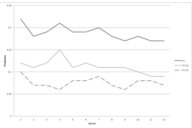
2-8 Frequency of price changes in each calendar month . . . 68

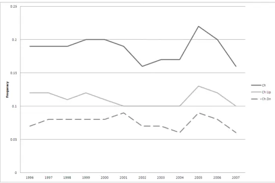
2-9 Frequency of price changes in each year . . . 69

2-10 Aggregate hazard function for consumer prices . . . 70

2-11 Hazard function for non-energy goods . . . 72

2-12 Hazard function for household service. . . 73

2-13 Comparison of ours and BE’s estimation of hazard function. . . 74

2-14 Distribution of durations across …rms. . . 75

(12)

2-16 Hazard function of price change in Calvo pricing. . . 86

2-17 Distribution of duration across …rms implied by Calvo model . . . 87

2-18 Simulation of price trajectory from Calvo model. . . 88

2-19 Real price and real cost simulated by Calvo model. . . 89

2-20 Hazard function of price change from menu cost model. . . 90

2-21 Distribution of duration across …rms implied by menu cost model. . . 91

2-22 Actual price trajectory, desired nominal price, and general price level sim-ulated from menu cost model. . . 93

2-23 Real price and real cost simulated by menu cost model. . . 94

2-24 Hazard function from Multiple Calvo model . . . 96

2-25 DAF from Multiple Calvo model . . . 97

2-26 Hazard function generated from Multiple Menu Costs model . . . 99

2-27 DAF generated from Multiple Menu Cost model . . . 100

3-1 Actual DAF vs. Minimum Duration 11 COICOP . . . 116

3-2 Actual DAF vs. Minimum Durations . . . 118

3-3 Calvo distributions at di¤erent levels of aggregation vs. Actual DAF. . . 121

3-4 IRF of money growth shock in Quantity Theory model for GTE price-setting.132 3-5 IRF of money growth shock in Quantity Theory model for GCE price-setting.133 3-6 IRF for monetary shock in the Smets and Wouters model with GTE price-setting. . . 136

(13)

3-7 IRF for monetary policy shock in the Smets and Wouters model with GCE

price-setting. . . 137

3-8 Quarterly distribution of duration across …rms. . . 140

3-9 Quarterly hazard functions comparison. . . 142

4-1 Unconditional hazard function . . . 167

4-2 Aggregate baseline hazard function . . . 183

(14)

Chapter 1

General Introduction

In this thesis, I intend to analyze nominal price rigidities under a uni…ed framework proposed by Dixon (2012), employing micro price data underlying CPI and PPI in the United Kingdom. I also attempt to reconcile micro and macro evidence, adopting a common general framework that allows for an explicit modeling of the distribution of contract lengths and for di¤erent types of price setting. I also evaluate how far the theories are consistent with the micro evidence on price rigidity. I investigate the …rm’s decision to change its price by developing a time-varying Ss band model, which allows evaluation of di¤erences across …rms and economic sectors in the hazard rate of price changes. In this chapter, I will provide a brief overview of the area of study explored in this thesis. The motivation behind the study will be outlined and introductions to the areas of research, the research questions and an insight into the structure of the thesis will be explored.

(15)

1.1

Research Background and Current Situation

The study of nominal price rigidities is "one of the hot topics of research in macro today". Blanchard (2009) highlighted the role of nominal rigidities in his paper of "The State of Macro":

The new-Keynesians...accepted the need for better foundations for the various imperfections underlying that approach. The research program became one of examining, theoretically and empirically, the nature and the reality of various imperfections, from nominal rigidities, to e¢ ciency wages, to credit market constraints.

There is a considerable amount of theoretical and empirical literature on nominal price rigidities.

1.1.1

Models of pricing

There are several theoretical approaches in the literature modelling nominal rigidities at the individual level. They are based on various assumptions for price non-adjustment: Calvo/Taylor type contract; menu costs, sticky information; customer anger. I will review the assumptions and implication of these pricing models, so as to check them against micro evidence and macro evidence.

Taylor/Calvo type model Nominal prices, according to Taylor (1980), are …xed by

(16)

time, duration of nominal prices remains constant for all .rms. In the Taylor model, prices are …xed for N periods and the hazard rate is zero for all duration except N; when the period is N, the hazard rate is one. Hence, the hazard rate is the measurement of likelihood of a price change depending on the elapsed duration of a price spell.

In the Calvo (1983) model, the probability of a price change is constant. Each period, a …xed proportion of …rms are able to change prices; the remaining …rms keep their nominal prices …xed. The probability of being able to change price is the same for all …rms, regardless of when they changed price last. This means that the hazard rate is constant.

The simple Taylor and Calvo type price setting models are inadequate in generating enough persistence of output and in‡ation to monetary policy shocks (e.g., Fuhrer and Moore, 1995, Chari et al.,2000, Christian et al., 2005).

One popular theoretical justi…cation is to add indexation to the Calvo model (e.g., Smets and Wouters 2003, Woodford 2003, Christiano et al. 2005). Price is set at the beginning of the contract, and for the contract duration this is updated by the previous period’s in‡ation. Though the Calvo with indexation can model in‡ation and output persistence well, it is at the cost of having prices changing every period.

Generalized Taylor (GT)1 _{model and Generalized Calvo model}2 _{are introduced to}

explain in‡ation and output persistence while being consistent with the microevidence on nominal rigidity. In GT model, there are many sectors with di¤erent price-spell

1_{See Taylor (1993), Coenen}_{et al} _{(2007), and Dixon and Kara (2010,2011), Dixon (2012) for details.} 2_{See Wolman (1999), Mash (2003), Sheedy (2007), Dixon (2012).}

(17)

lengths, and within each sector there is a simple Taylor process. In GC model, the reset probability is duration-dependent. Additionally, we can model the price setting strategy as a multiple sector Calvo model (MC), which is special case of GC3_{. A key feature of these}

generalized models is that they re‡ect the substantial heterogeneity observed in micro data. Price rigidity varies across sectors. In the presence of pricing complementarities the slow adjusting sectors have a disproportionally large e¤ect on overall price adjustment, slowing the price response, and increasing the output response to shocks. The intuition is as follows. When a heterogeneous economy is hit by a shock, the initial adjustment takes place by …rms mostly in the fast adjusting sectors. As time passes, a large proportion of …rms that still have to adjust are …rms in the slow-adjusting sector. In other words, the adjustment process is dominated initially by high frequency adjusters and later by low frequency adjusters. Furthermore, the presence of slow adjusting sectors and strategic complementarities slows down price adjustment in the fast adjusting sectors.

As supposed by Dixon (2012), we can link the GT with micro data by looking at the cross-sectional distribution of duration across …rms, and link the GC to the micro data through the hazard function. Moreover, MC can be linked to micro data by looking at the frequency of price changes at sectoral level.

(18)

Menu costs

The menu costs model assumes that the price change is costly and these costs prevent …rms from changing prices in a continuous manner. Sheshinski and Weiss (1977) show that in presence of price changing costs, the optimal pricing policy is of the (S,s) type. The S and s indicate the upper and lower bound for the real price, respectively. Once the real price lies within the bounds, the nominal price will be kept constant. Over the pricing period, the optimal policy is a kind of state-contingent policy.

Under state-contingent policy, …rms adjust prices within a relative large range due to the fact that the current prices had been deviated from the optimal price. That the aggregate price level will be adjusted more rapidly to nominal changes is resulted from the selection e¤ect, in particular, when …rms are constrained by state-contingent instead of time-contingent pricing. Monetary shocks have been evidenced to have longer lasting real output e¤ect in time-dependent (i.e. Calvo) models than in menu costs model4_{. In}

addition, monetary impulses make prices elicit more rapid response in menu costs models than in time-dependent models.

The menu costs models are usually solved using numerical methods, so no analyti-cal expression is available for the hazard rate. In most analyti-calibrations made by previous researchers, the hazard is increasing with the duration.

4_{See Caplin and Spulber (1987), Dotsey et al. (1999), Gertler and Leahy (2006), and Golosov and}

(19)

Sticky information

It is assumed that it is costly for …rms to gather information about the current economic conditions (Mankiw and Reis, 2002). Fischer (1977) pointed out those opportunities to adopt new price paths had been evidenced to arise stochastically. New information about the state of the economy has been adopted and a new path of optimal prices has been updated each period. Outdated information is used to make pricing decisions by the rest of …rms. In‡ation, therefore, depends on previous expectations of current in‡ation and output.

Because substantially larger and persistent real e¤ects are resulted from monetary shocks, the sticky information model …t macroeconomic facts better. However, in absence of other frictions, some form of indexation no matter it is to the general, sectoral or price level is involved in …rms’optimal price plans in absence of other frictions. Therefore, all …rms change price all the time in sticky information model. This argument, however, is contradictory to empirical evidence based on micro economic data. Prior studies make attempts to solve this problem by combining sticky information with menu costs (Klenow and Willis, 2006; Knotek, 2006). Using both assumptions, namely, sticky information and menu costs, causes two consequences: prices are not constantly changed; and old aggregate level in‡ation innovations will be re‡ected by the new prices when both as-sumptions change. This is due to the fact that price changes are not in accordance with getting informed about the state of the economy. Knoteck (2006) suggested that the micro features of the economy can be inferred by adjusting parameters to match general

(20)

macroeconomic behaviour. He found that information is updated once every 7 quarters typically; price is changed once every 2 quarters; and 10% of prices remain unchanged for more than 2 years. An economy in which …rm face both menu costs and a cost of knowing macroeconomic conditions needs to be considered (Gorodnichenko, 2008). Two methods that …rms can adopt to get information either paying the costs or by learning the actions of other .rms. This results in an information externality and encourages …rms delay their price adjustment. Following a shock, price adjustment is postponed because …rms expect to catch the chance to observe other …rm’s actions in order to achieve better pricing choice. As a result, in‡ation responds to nominal shocks slowly and the response is hump-shaped, and in‡ation is persistent.

Customer anger

Rotemberg (2005) develops a model to explain the price rigidity. This model indicates that consumers analyse …rms’pricing decision depending on the perception of fairness. If consumers are convinced that price are unfair, they will have adverse reaction towards relevant products or services. Hence, …rms may reluctant to change prices to avoid potential anger. Chances are that …rms keep prices the same even if they desire to change prices due to the fact that price changing will elicit consumers’evaluation of fairness of prices and cause potential negative reactions. Overall, …rms respond to macroeconomics conditions and change prices. For example, consumers are unlikely to have negative reaction and accept prices change under the circumstances of rapid in‡ation. In addition,

(21)

customers who are heterogeneous in information holding will have various responses to price changing. Firms will change the prices within di¤erent time schedule pertinent to the development of consumers beliefs.

1.1.2

Empirical studies

Micro price studies have been conducted using di¤erent sources of data, such as the micro data underlying national CPIs and PPIs, sub-national store scanner data, "scraping" prices from internet, and the survey data. A set of stylized facts have been found in empirical analyses. They are summarized as following5:

Prices change infrequently

Dhyne et al. (2006) …nd that the monthly frequency of consumer price change is about 15% in the euro area. Excluding the countries with the highest and the lowest frequency, the resulting frequency of price changes is 16.9%. The implied average duration, which equals to the inverse of frequency, is about a year. Vermeulen et al. (2006) show that the average frequency of producer price change is 21% in the euro area. Bils and Klenow (2004) report that the average frequency of consumer price change in the US for 1995-1997 period is 26.1%; While Klenow and Kryvtsov (2008) …nd that the monthly frequency of the US consumer price change is 29.3% between 1998 and 2003.

Sales are common in the US consumer price data, the share of sales prices in the US

5_{This study mainly reviews the empirical …nding from using CPI and PPI micro data in the US and}

(22)

CPI data is about 20%. Speci…cally, Nakamura and Steinsson (2008) de…ne sale as a situation in which a price falls temporarily and then returns to the price in e¤ect just before the decrease, and in such situation no regular price change is recorded. There are some other methods to identify sales. For example, Kehoe and Midrigan (2007) indicates a sale if "price decrease is followed by any price increase thereafter". Nakamura and Steinsson (2008) …nd that after excluding the sale prices, the median frequency of the US consumer prices is 11.1% in 1988-1997, and 8.7% in 1998-2005.

Substitutions are observed in many sectors. Nakamura and Steinsson (2008) report that the monthly rate of forced item substitution is about 10 percent in "Apparel" and "Transportation Goods", and about 6 percent in "Recreation Groups". Klenow and Willis (2007) estimate that price changes associated with item substitutions are sensitive to in‡ation. However, the …ndings of Klenow and Willis (2007) depend to some degree on their modeling assumptions.

The frequency of price changes varies across sectors

Dhyne et al. (2006) document the heterogeneity with respect to frequency of consumer price changes across sectors in the euro area. The frequency of price changes ranges from 5.6% in "Services" to 28.3% in "Unprocessed Food" and 78% in "Oil Products". Nakamura and Steinsson (2008) report the distribution of the frequency of price changes for about 300 Entry Level Items (ELI). The ELI with the highest frequency of price changes, 100%, is "Used Cars". The ELI with the lowest frequency of price changes,

(23)

1.6%, is "Legal Services".

The micro data show that, in the real world, there are many heterogeneous …rms. In general, a macro model with a "representative …rm" does not behave like a model with many heterogeneous …rms. One can construct and calibrate a model with a representative …rm and compare selected predictions of this model to a version of the same model with many heterogeneous …rms. If the predictions from the representative …rm model come close to those obtained from heterogeneous …rm model, then the predictions of the representative …rm model are reliable.

Price decreases are common

Dhyne et al. (2006) report that 42% of price changes are decreases in the euro area. While Nakamura and Steinsson (2008) …nd this fraction to be roughly one-third in both consumer prices excluding sales and …nished-goods producer prices. Food and energy price increases and decreases are almost equally likely. For industrial goods 43% price changes are decreases. Price decreases are less common for services, for which they constitute only 20% of price changes. However, micro data suggest that there is no stronger downward nominal price stickiness.

The …nding that price decreases are common has important implications for the cal-ibration of models of price rigidity. As shown in Nakamura and Steinsson (2008), the fraction of price changes that are decreases helps to pin down the key parameters in a benchmark menu costs model along the lines of Golosov and Lucas (2007). It also

(24)

provides strong evidence for the hypothesis that idiosyncratic shocks are an important driving force for price changes.

Downward sloping hazard function

A "dynamic" feature that has been documented in many studies is the shape of the hazard function of price change. The general …nding in the literature is that hazard function is decreasing. Alvarez (2008) reports that the frequency of price changes conditional on reaching a given age is downward sloping when all goods are considered together, but note that this could be the consequence of heterogeneity in the probability of price adjustment. For a price changed recently there is a high likelihood that the good is a ‡exible price good and so the probability of the occurrence of a price change is high; for a price that has been unchanged for a long time it is likely that the good is a sticky price good and the probability of price change is low. This is so called "selection e¤ect". Hence the empirical hazard rate is downward sloping.

Nakamura and Steinsson (2008) estimate the hazard function of price change for consumer and producer prices, controlling for heterogeneity across products. The hazard functions are downward sloping for the …rst few months, then mostly ‡at except for a large twelve-month spike in all major groups. Accounting for heterogeneity leads to a substantial ‡attening of the hazard function. But they do not …nd evidence to support for upward sloping hazard function. Furthermore, they suggest that menu costs model can generate a variety of shapes of hazard functions, depending on the relative importance

(25)

of transitory and permanent shocks to marginal costs. Firms may be more attentive to getting prices right when revenue is temporarily high for a product due to idiosyncratic supply or demand considerations. Large idiosyncratic shocks tend to produce a downward sloping hazard.

1.1.3

Summary

Previous research has demonstrated the importance of assessing the nominal price rigidity using micro data. The stylized facts obtained from micro data can help us to examine pricing behaviour at the …rm level, where pricing decisions are actually made. Individual information on price setting allows determining to which extent the assumptions used in deriving theoretical models are actually realistic, which helps re…ne modeling strategies.

1.2

Research objectives

My thesis consists of three individual essays which all shed light on assessing the price rigidity by using price micro data in the UK. The relevant implications for macro models are also discussed in each essay respectively. My thesis mainly focuses on a few research questions shown as follows:

1. How often do consumer prices change?

2. How can we deal with the censoring and sampling issue when the hazard function is estimated from the UK CPI micro data?

(26)

3. Would the probability of price change vary along the duration of price spells? 4. How can we derive the distribution across …rms which is consistent with a given

mean frequency of price changes?

5. Whether the workhorse pricing models can …t the empirical evidence in micro data, if not, what can be done to re…ne modeling strategies?

6. What is the minimum (maximum) mean duration of price-spells averaged across …rms consistent with a given frequency of price changes?

7. Can we just use frequencies of price change to generate corresponding hypothetical distributions which can match the "true" distribution across …rms?

8. Do the DSGE models under the Calvo distribution hypothesis behave in a way similar to models calibrated with the microdata ("true" DAF)?

9. How can we build a time-varying Ss model which has implication consistent with the micro evidence found in the UK PPI micro data?

10. How can we evaluate the e¤ects of covariates on the hazard rate?

11. How can we control for the unobservable heterogeneity when hazard function is estimated?

1.3

Research outline

(27)

In Chapter 2, I assess the price rigidity in a uni…ed frameworka la Dixon (2012), using CPI micro data in the UK. I estimate the frequency of price change, given the information about sales and substitutions. I give a detailed discussion about the e¤ect of censoring and sampling on the estimation of hazard function. I derive the distribution across …rms which are consistent with a given mean frequency of price changes in terms of the corresponding proportion of …rms resetting prices. I exam pricing behaviour of two benchmark pricing models: menu costs and Calvo. And I build models with heterogeneous structure in price setting to improve models’…tness in respect to matching microevidence.

In Chapter 3, I seek to analyze how much the frequency could tie down the behaviour of …rms in steady-state in terms of the average length of price spells across …rms. I derive an upper and lower bound for the mean duration of price-spells averaged across …rms. Then the UK CPI micro data at the aggregate and sectoral level are used to …nd that the actual mean is about twice the theoretical minimum consistent with the observed frequency. I estimate the distribution using the hazard function and …nd that although the estimated hazard di¤ers signi…cantly from the Calvo distribution, the means and medians are similar. However, despite the micro di¤erences, I …nd that the arti…cial Calvo distributions generated using the sectoral frequencies result in very similar impulse responses to the estimated hazard when used in the Smets-Wouters (2003) model.

In Chapter 4, I examine the behaviour of individual producer prices in the UK. A number of stylized facts about price setting behaviour are uncovered. The weighted average frequency of price change is 25%, and there are about 44% of price adjustments

(28)

are price decreases. The frequency of price changes varies substantially across industry groups and product sectors. The unconditional hazard function displays a downward sloping pattern with annual spikes. Then I set up a time-varying Ss model which is consistent with the micro evidence. Then a duration model is speci…ed according to the Ss model. I estimate the duration model which controls for observable and unobservable heterogeneity across …rms in assessing the e¤ect of changes in in‡ation, interest rate, oil price, industrial output, and exchange rate on the hazard rate of price changes.

In Chapter 5, I discuss the major …ndings of this research. I also discuss the limitations of this research and suggest areas for future research.

(29)

Chapter 2

Frequency, Hazard Function, and

Distribution across Firms

2.1

Introduction

In monetary macroeconomics, the price rigidity plays a key role in many models’setup. Not only it a¤ects the "real e¤ect" of monetary policy and the dynamic of in‡ation, but it also has a deep in‡uence on optimal monetary policy. There are quite a few important questions which need to be addressed in the micro price data set, such as: how often do the consumer price and/or producer price change, would the probability of price change vary along the duration of price spell, and what does the distribution of price durations look like? Furthermore, we would like to investigate whether the workhorse pricing models can …t the empirical evidence in micro price data. In this chapter, we intend to

(30)

indicate the stylized facts of the price setting mechanism in the UK economy, and take important steps at discriminating among models by assessing the ability of "two of the most popular models of price rigidity"–the Calvo and menu costs models –to match key empirical features of …rm’s price-setting behaviour we found in the UK CPI micro data. Price stickiness has been studied at the level of individual …rms since 1920s. Mills (1927) and Means (1935) distinguish two types of products: the one with ‡exible price, and the other one with "administered price", and they …nd that many prices change infrequently and the frequency of price changes varies widely across goods. Their work has spurred a voluminous literature. Early studies mainly focus on price adjustment for particular products. Mussa (1981) and Weiss (1993) describe the behavior of newspaper prices during the 1920s German hyperin‡ation. Carlton (1986) …nds evidence on the dynamics of industrial prices. Cecchetti (1986) investigates the magazine cover prices. Lach and Tsiddon (1992) study the behavior of the prices of 26 foodstu¤s at grocery store in Israel. Kashyap (1995) checks the catalogue product.

Recently, many researchers broaden the source of micro price data. Blinder et al (1998) make surveys of …rm managers. Eichenbaum, Jaimovich and Rebelo (2011) use scanner data from supermarkets, drugstores, and mass merchandisers in the U.S. Cavallo (2009) collects the online-shopping price data in Brazil.

Date sets underlying o¢ cial CPIs have become available to researchers since new millennium. For the U.S., the leading research was conducted by Bils and Klenow (2004). In their in‡uential work, they focus on the micro-data of CPIs between 1995 and 1997

(31)

in U.S. They …nd that the price rigidity is not serious. On average, the price can remain the same for 3 to 4 months, which is much shorter than the estimate from macro model. Klenow and Kryvtsov (2008), Nakamura and Steinsson (2008) both extend the work of Bils and Klenow (2004) in di¤erent directions. Nakamura and Steinsson (2008) not only investigate the CPI micro data, but also do the thorough research on PPI micro data. For the euro area, Dhyne et al. (2006) have a good summary of all the related work done by the members of In‡ation Persistence Network1_{. For the United Kingdom, Bunn and Ellis}

(2012a) (BE hereafter) is the …rst trial. Our study di¤ers from BE from three aspects. First, we assess the price rigidity in a uni…ed framework, which includes frequency, hazard function, and distribution across …rms. Second, we estimate the hazard function using all the normal (uncensored) and right-censored price spells. Whereas BE only choose one complete price spell for each item to estimate the hazard function. We point out that not only this method su¤ers the loss of important information from discarding large amount of spells, but also faces the problem of selection bias. Third, we derive out the distribution of durations across …rms. And we argue that the cross-sectional feature of price setting behaviour is important to make macro-model …t the micro-evidence, as suggested by Dixon and Kara(2010).

Individual …rms do not continuously adjust their prices in response to shocks that hit

1_{For the other countries: Baharad and Eden (2004) point out that the popular method adopted}

by most researchers su¤er the over-sampling bias. They announce a method to correct the downward bias in estimation of price rigidity. Gagnon (2007) investigates the price rigidity for Mexico during the hyperin‡ation period. Kovanen (2006) gets the result for Sierra Leone; Goueva (2007) has the estimation of price rigidity for Brazil; Masahiro and Saita (2007) report the conclusion for Japan; Hofstetter (2010) provides evidence on how often prices change in Colombia.

(32)

the economy. To model this fact, the economic literature considers mainly two types of pricing behaviour: time dependent and state dependent pricing rules. According to the former, …rms are assumed to change their prices periodically using either a deterministic (Taylor, 1980) or a stochastic (Calvo, 1983) process of price adjustment. More speci…cally, in the Calvo model, …rms face a probability of optimizing their price, which is exogenous and constant. Therefore, the timing of the price changes is exogenous and does not depend either on the timing of the shocks or on the state of the economy. Due to its tractability, the Calvo model enjoys popularity in the macroeconomic literature.

Firms following state-dependent pricing rules are usually assumed to review their prices whenever relevant shocks hit the economy but, due to the existence of …xed costs of changing prices (e.g., the costs of printing and distributing new price lists), they change their prices only when the di¤erence between the actual and target prices is large enough (see, for example, Sheshinski and Weiss, 1977, Caplin and Spulber, 1987, Caballero and Engel, 1993, Dotsey et al., 1999). Thus, a company facing these menu costs will change its price less frequently than an otherwise identical …rm without such costs.

There are debates on how to embed price stickiness inside macroeconomic models, and whether one can construct a price-setting model consistent with the micro evidence that has plausible macroeconomic implications.

In this chapter we examine the frequency of price changes underlying the UK CPI micro data, with the consideration on the e¤ect of sales and substitutions. The major aim is to analyze the degree of the nominal rigidity present in United Kingdom consumer

(33)

prices and trying to applying a uni…ed framework (proposed by Dixon, 2012) to study the characteristics in price setting behaviour.

We …nd that the monthly average frequency of price changes is 19 percent for identical items in CPI micro data. Moreover, the frequency of price changes varies considerably across sectors and products. For various fuel types and seasonal food products the average frequency can be as high as 90 percent per month. However, for several services and administered prices, such as automatic car wash, and digital photo printing, the frequency can be as low as 3 percent per month. To provide a measure of distribution of price durations across …rms, we estimate the aggregate hazard function for all price spells. Similar to previous studies, we …nd that the aggregate hazard function is decreasing with most marked annual spike. We derive the distribution of durations across …rms from the hazard function. In line with previous studies (Baharad and Eden 2004, Dixon 2009), the distribution of duration across …rms has fatter long tail than the distribution of duration across contract, indicating that the price is stickier than we thought. Moreover, the "stickier" sectors dominate the behaviour of in‡ation in the longer term.

The potential contributions of this chapter are three folds: we …rstly take empirical study of price rigidity under the framework of distribution across …rms. A uni…ed frame-work for using micro-data a la Dixon (2012) combines frequency method with hazard function, and then derives the distribution across …rms (hereafter DAF). Secondly, we in-vestigate the censoring issue in detail, and discuss the di¤erent e¤ect on the estimation of hazard function resulted from di¤erent method on dealing with right-censoring. Thirdly,

(34)

we calibrate a benchmark menu costs model and Calvo model to match the evidence we obtained from micro-data, and we check the implication of di¤erent pricing models with heterogeneous structure.

The structure of the chapter is allocated as following: Section 2 provides the data description and some speci…c data issues; Section 3 discusses the methodology used in assessing price rigidity, pointing out the connection among frequency, hazard function and DAF; Section 4 provides the empirical results we get from CPI micro data; Section 5 maps micro-evidence with macro model; Section 6 provides possible extension to the benchmark pricing model; and in Section 7 we conclude.

2.2

Data

2.2.1

Date description

The micro data used in this paper are produced by the O¢ ce of National Statistics (ONS hereafter), Because of the con…dentiality issues relating to information collected about individual …rms, it is not possible to makes this type of data widely available. The micro data that underlie the consumer and producer price indices used in this research were made accessible via the VML2.

2_{This work contains statistical data from ONS which is Crown copyright and reproduced with the}

permission of the controller of HMSO and Queen’s Printer for Scotland. The use of the ONS statistical data in this work does not imply the endorsement of the ONS in relation to the interpretation or analysis of the statistical data. This work uses research data sets which may not exactly reproduce National Statistics aggregates.

(35)

2.2.2

CPI data

The ONS collect a longitudinal micro data set of monthly price quotes from over ten thousands of outlets to compute the national index of consumer prices. There are two basic price collection methods: local and central. Local collection is used for most items. There are about 150 locations around country, and around 120,000 quotations are ob-tained each month by local collection. For some items, collection in individual shops across the 150 areas is not required- for example, for larger chain stores who have a national pricing policy or where the price is the same for all UK residents or the regional variation in prices can be collected centrally. Central collected data cover about 33% of CPI, but they are not available to our research3_{. Therefore, our CPI research data mainly}

are local collected, covering about two thirds of total CPI. The sample spans over the time period from January 1996 to December 2007 and contains between 112,676 (1996) and 99,524 (2007) elementary price quotations per month. And our data sample includes over 14 million observations. The coverage and classi…cation of the CPI indices are based on the international classi…cation system for household consumption expenditures known as COICOP (classi…cation of individual consumption by purpose). This is a hierarchical classi…cation system comprising: divisions e.g. 01 Food and non-alcoholic beverages, groups e.g. 01.1 Food, and classes (the lowest published level) e.g. 01.1.1 Bread and

3_{The sample excludes 33% of CPI items which are central collected. The central collected data set}

include price quotes for education, some of the energy goods, and some of the communication services. However, we don’t have the detail of the description. We do recognize the potential sample selection bias. But the data availability is the most common issue in this kind of micro price data research. And we argue that we have the most representative data set so far to ful…l our research objectives.

(36)

COICOP division Freq. Percent Cum.

Food and Non-Alcoholic Beverages 25,191.51 17.62 17.62

Alcoholic Beverages and Tobacco 10,083.28 7.05 24.67

Clothing and Footwear 13,323.33 9.32 33.98

Housing and Utilties 9,350.23 6.54 40.52

Furniture and Home Maintenance 16,211.75 11.34 51.86

Health 2,705.55 1.89 53.75

Transport 14,800.15 10.35 64.1

Communications 237.2797 0.17 64.27

Recreation and Culture 14,085.51 9.85 74.12

Education 6.340364 0 74.12

Restaurants and Hotels 25,087.06 17.54 91.67

Miscellaneous Goods and Services 11,918.02 8.33 100

Total 143,000 100

Table 2.1: CPI share in COICOP sectors

cereals. As table 2.1 shows4_{, the division Food and non-alcoholic beverages accounts for}

about 17% of the CPI weight in the subsample available in the dataset. The education division is excluded from our research due to the lack of observation.

In our CPI research data set, each individual price quote consists of information on the item code, the outlet, the region, the date and etc. And we de…ne the product category at the elementary level, for example, an item could be indicated as large loaf, white, unsliced (800g). There are a total of675 products categories in our raw dataset, and the product varies by its speci…c variety and brand with each product category. However, the data set has been anonymized with respect to the variety and brand of the product.

4_{Similar to the situation illustrated in Bunn and Ellis (2012a), only the locally collected data that}

account for about two thirds of the CPI are available. While centrally collected data are not available for the research. Therefore, the average weights in this study do not equal to the average weights underlying o¢ cial CPI. This is in line with the …nding in Bunn and Ellis (2012a, Figure 1). Speci…cally, the average weight of Food and Non-Alcoholic Beverages in this study is about 17%, which is higher than the average published CPI weight (about 12%) ; the average weight of Communication is this study is less than 1%, while the average published CPI weight is about 2%.

(37)

With the information on the item i, the shop j, the location k, and the date t, we can construct a price trajectory Pijk;t, which is sequence of price quotes for a speci…c item belonging to a product category in a speci…c shop over time. Speci…cally, we take two sequential price quotes belong to the same price trajectory if they have the same product identity, location and shop code. There are about 614;000 price trajectories. And the average length of each price trajectory is about 24months.

As Table 2.2 described, the average length of price trajectory di¤ers quite a lot among di¤erent COICOP sectors. The sector with longest price trajectory in average is health sector, indicating that the item belonging to health sector appear in CPI research data as long as two and a half year. On contrary, an item in the communication sector usually disappears from our CPI basket after one and a half year. It shows that the communication sector is updated more frequently in CPI basket.

Furthermore, we can de…ne a price spell as the sequence of price quotes with the same price for a speci…c item in a speci…c shop. The length of price spell (duration) is a key factor when we assess the price rigidity. Moreover, the distribution of duration will provide us a possible perspective to model the price rigidity. We will try to measure the average length (duration) of price spell and get the distribution of duration in following sector.

(38)

COICOP Sector Mean length of price trajectory

Median length of price trajectory Food and Non-Alcoholic

Beverages

26.0 21

Alcoholic Beverages and Tobacco

28.6 22

Clothing and Footwear 19.6 13

Housing and Utilties 25.2 21

Furniture and Home

Maintenance

24.5 19

Health 30.1 23

Transport 26.7 23

Communications 18.7 12

Recreation and Culture 23.3 19

Education na na

Restaurants and Hotels 25.3 23

Miscellaneous Goods and Services

26.1 22

Table 2.2: Average length of price trajectory by COICOP sector

2.2.3

Speci…c data issues

Censoring

Censoring is a word often used in survival analysis literature, which is de…ned as a situation when the failure event occurs and the subject is not under observation. In this paper, a failure event is speci…ed as a price change. Suppose that the surveys sample individual price quote between the date B and E (as in Figure2-1. The date B is the beginning of the survey period, while date E is the ending of it. We de…ne a normal price spell as the period between two price changes. Censoring occurs when you are prevented from seeing the exact time of the failure event (price change, in our context).Therefore, censoring entails a downward bias in the estimation of the duration of price spells, as

(39)

longer price spells are more likely to be censored. In general, we can classify the price spells into four groups with di¤erent censoring type as shown in Figure2-1:

1. Non-censored price spell, or normal price spell: we can observe the beginning and ending of the price spell explicitly, which can be seen as S1 in Figure2-1

2. Left-censored price spell: if we do not know the true starting date of the price spell. This usually happens when new item or product is introduced to CPI basket. S2 in Figure2-1 gives an example. Spells such as S4 may be recorded as a duration beginning at B and lasting until the completion of the spell, in which case the actual duration is unknown since the time from the inception of the spell to the beginning of survey (B) is unknown.

3. Right-censored price spell: if we do not know the ending date of the price spell. E.g. a product withdraws prematurely; a product no longer be available in an outlet, or the outlet shut down; or at the end of sample period. We can illustrate this type of spell as S3 in Figure2-1.

4. Double-censored price spell: as shown as S4 in Figure2-1,if both the start and the end of the spell is not observed, i.e. the price spell of the product actually begins before the statistical agency starts to observe the product, and ends after the statistical agency stops to observe the product.

We can summarize the reasons which can explain the censored price spells in our observations. First, the observation period is restricted by the database availability.

(40)

Figure 2-1: Type of price spells

This makes it very likely to observe product prices in a given outlet after the current price of the product was actually set and/or before that price ceases to exist. Indeed, the probability that the …rst spell in a price trajectory is left-censored is high, as is one of the last spell being right-censored. Second, the sampling of products and outlets by the statistical agency is also likely to generate some censoring. Indeed, the statistical institute may decide to discard a speci…c product from the "representative" CPI basket due to changes in technology or consumer behavior that shrink the expenditure share on these products (e.g. black and white TV sets) although they may still be sold in outlets. Then,

(41)

the last price spell of such a product will be right-censored. Conversely, products may be included in the CPI basket and their price observed after they were actually available for consumers. This will generate left-censoring of the price spell. Third, outlets and …rms may decide to stop selling a product which price was followed by the statistical agency. Then, the procedure which is often adopted by statistical agencies in charge of computing the CPI consists in replacing the "old product" by another one, either a close substitute in the same outlet or the same product but in another outlet. It is then very likely that the price of the "replacing product" was set before the …rst price observation for this product. We then have left-censoring of the price spell for this new product.

In our CPI data set, there are over 3 million price spells. The majority of price spells are uncensored, covering 42% of whole sample; the share of left-censored price spells is 20%; the share of right-censored price spells is 30%; and the share of double-censored price spells is 8%5_.

Sales

Nakamura and Steinsson (2008) suggest that temporary sales have "strikingly di¤erent macroeconomic implications". Guimaraes and Sheedy (2011) point out that sales have important implication on monetary policy. The ONS gathers consumer price data on whether a product was "on sale" or "recovering from sale" when its price was sampled in a particular month. Sales prices are recorded if they are temporary reductions on

5_{Double censored price spells are 8% of the sample. However, it does not mean that 8% of prices were}

(42)

goods likely to be available again at normal prices or end of season reductions. Prices in closing down sales and for special purchase of end of range, damaged, shop soiled or defective goods are not recorded as they are deemed not to be the same quality as, or comparable with, goods previously priced or those likely to be available in future. We identify temporary "sales" with the ‡ag provided by ONS6. However, alternative "sales" …lters are proposed by other researchers. There are three kinds of price …lters used by previous studies:

1. The AC Neilsen …lter, which is used by Kehoe and Midrigan (2007) (KM hereafter), indicates a sale if "price decrease is followed by any price increase thereafter".

2. Nakamura and Steinsson (2008) (NK hereafter)suggest a sale …lter that ‡ag a sale only when a price decrease is followed by a return to the price in e¤ect just before the decrease.

3. Eichenbaum, Jaimovich and Rebelo (2010) (EJR hereafter) identify the most fre-quently observed price in a given quarter as "reference price", which means that it excludes an even larger portion of price changes than sale …lters, yielding "more persistent series and suggesting a stronger role for nominal rigidities."7

The EJR …lter restricts regular prices to change only on certain dates, and therefore greatly increases estimates of price persistence. The KM …lter is much more likely to

6_{All the discounting available for all customers are recorded by ONS, labelled as sale. While}

dis-counting only available for loyalty card members are not recorded by ONS.

7_{Chahrour (2010) proposes a new price …lter similar to the EJR (2010) and show that implications}

(43)

records a sale even if it is a reversion in regular price, and therefore it may identify spurious sales. The NS …lter is more strict, which will typically identify fewer sales and more frequent price changes. We choose NS …lter to identify the "sales", however, the empirical …nding suggests that there is trivial di¤erence between NS …lter and ONS’sale ‡ag. Furthermore, we …nd that sales have some kind of "seasonal pattern", which can be shown in Figure 2-2.

Figure 2-2: Sales as percentage of total price quotes in each calendar month

Concerning the price changes associated to sales we decided to follow a dual approach: In the baseline version of the results we treat sales as regular price changes which ter-minate a price spell. However, it can be argued that these price changes merely re‡ect noise in the price setting process and are not due to changes in fundamental price

(44)

deter-mining factors (as e.g. monetary policy and business cycle developments) and therefore they should be ignored from the viewpoint of monetary policy analysis8. Therefore, we also provide an alternative set of results without taking into account the price changes induced by sales. In order to exclude price changes induced by ‡agged sales from our analysis, we replace all ‡agged sales prices with the last regular price9, i.e. the price before the sale started.

The sales price quotes account for about 7% of whole sample10_{. It is lower than the}

share of sales prices in the US CPI data, which account for about 20% (Nakamura and Steinsson,2008). There is signi…cant di¤erence in our estimation of price rigidity if we choose to include or exclude sales data.

Substitutions

Nakamura and Steinsson (2008) claim that the importance of substitution draws “atten-tion to the ques“atten-tion of whether the relative frequency of di¤erent types of price changes is an important determinant of the macroeconomic implications of price rigidity”.As a measure of price change alone, the CPI should re‡ect the cost of buying a …xed basket of goods and services of constant quality. However, products often disappear or are

re-8_{However, Guimaraes and Sheedy (2007) argue that even if …rms can adjust sales without cost,}

monetary policy has large real e¤ects owing to sales being strategic substitution. Thus the ‡exibility seen in individual prices due to sales does not translate into ‡exibility of the aggregate price level.

9_{However, Eichenbaum et al. (2009) replace sale prices with reference prices which de…ned as the}

most common prices within a given quarter.

10_{Some authors, e.g. Baumgartner et al 2005, argue that the reporting of sales is generally up to the}

interviewer and therefore cannot be expected to be complete and consistent across all products. They additionally de…ne a "v-shaped" sale indicator. However, this …lter generates substantial fraction of sales when prices are perfectly ‡exible.

(45)

placed with new versions of a di¤erent quality or speci…cation, and brand new products also become available. When such a situation arises, direct comparison is adopted. If there is another product which is directly comparable (that is, it is so similar to the old one that it can be assumed to have the same base price), for example a garment identical except that it is a di¤erent colour, then the new one directly replaces the old one and its base price remains the same. This is described as "obtaining a replacement which may be treated as essentially identical" (CPI Technical Manual,2007), and is equivalent to saying that any di¤erence in price level between the new and the old product is entirely due to price change and not quality di¤erences. In CPI data, such "comparable" substitution is not uncommon. It accounts for a little more than 4 percent of our total CPI research dataset. The substitution happens more likely in the January, August, and September. This partially re‡ects the fact that ONS adjust the basket of CPI in the beginning of the year. Beside, the clothing and footwear are more likely to change the style when summer ends. We can show the substitutions as percentage in whole price quotes in each calendar month as Figure 2-3.

Outliers

We remove some price quotes from the data set mainly because they display unrealistic price movements. We set a very large pre-de…ned threshold value. Any individual price changes exceed this value will be detected as outliers and excluded from our study. We don’t want to apply a harsh …lter here. Therefore, only if individual price changes with

(46)

Figure 2-3: Substitution as percentage of total price quotes in each calendar month

(Pijk;t Pijk;t 1)=Pijk;t 1 > 100 will be de…ned as outliers. This is such a conservative

rule that only a few observations have to be discarded. The percentage of the exclusion is very trivial, less than 0.01%. Robustness checks have done on frequency of price changes. And it does not alter our result. However, it will a¤ect the mean size of price changes in some speci…c time periods for a few speci…c items. Though we do not focus on the magnitude of price changes. We only exclude the zero price quotes (prices dropping to zero) as outlier. Once again, the data treatment does not alter our results on frequencies of price changes.

(47)

Data Gaps

After removing the outliers from our data set, we faces the gaps in our data set. Specif-ically, the price quotes for some items are missing during some periods. This situation would be even worse when we exclude the sales and substitutions from our data set. We have to …ll the gaps when we estimate the duration of price spells. Therefore, we adopt a "carry forward" strategy. In another word, we will …ll the gaps with the last observable price. This strategy is consistent with Klenow and Kryvtsov (2008). But it will generate upward bias in estimating the duration of price spells. In order to make this potential bias as small as possible, we add another restriction when we adopt the "carry forward" strategy. That is, we only …ll the gaps not longer than 3 months. If the gaps are longer than 3 months, we consider the later one be a new price spell. This 3-month window is also used by Nakamura and Steinsson (2008) when they construct their own sale …lter. Alternative treatment would be treating the missing data as “loss”. Then this would e¤ectively increase the right censoring and left censoring observations, but to a very slightly higher level (less than 1%). However, our results are not signi…cantly a¤ected.

Weights

In CPI dataset, each individual price quote is attached with weight, which is given by ONS. The CPI weights cover monetary expenditure within the UK on goods and services. The weights are based on expenditure within the domestic territory by all

(48)

private households, foreign visitors to the UK and residents of institutions. The individual weights11 which initially do not sum to one as not 100 percent of the CPI is covered in our sample, are then rescaled such that the sum of the weights equals one and the relative weights among the goods are preserved.

2.3

A uni…ed framework in assessing price rigidity

In this section, we provide a uni…ed framework in assessing price rigidity from three perspectives: the frequency, the hazard function method, and the distribution of duration across …rms.

2.3.1

Frequency

The frequency of price changes is given for each product as the number of price changes in each period over the total number of price quotes for that product in that period. We assume that the proportion of …rms resetting price corresponds to the proportion of prices changing. It imply that each price trajectory corresponds to a di¤erent …rm. We

11_{The weights are used at the “item” level, which is the most disaggregated level. More speci…cally,}

(49)

can use dummies Ij;t to de…ne the price change12: 8 > > < > > : Ij;t = 0 if Pj;t =Pj;t 1 Ij;t = 1 if Pj;t 6=Pj;t 1

where Pj;t and Pj;t 1 belong to the same trajectory. Similarly, we can de…ne the price

increase/decrease with dummies: 8 > > < > > : Uj;t = 1 if Ij;t = 1&Pj;t > Pj;t 1 Uj;t= 0 all else 8 > > < > > : Dj;t = 1 if Ij;t = 1&Pj;t < Pj;t 1 Dj;t = 0 all else

And the weighted average frequency of price changes is de…ned as

f = PT t=1 PJ j=1!j;tIj;t PT t=1 PJ j=1!j;t ;

The frequency approach now is standard in the empirical sticky-price literature13. It has following advantages:

12_{This is a kind of backward comparing scheme. This method is used by a lot of researchers, such as}

Fougere et al. (2007), Nakamura and Steinsson (2008), Bunn and Ellis (2012a). The price change can also be de…ned in a forward comparing way. However, we argue that when sample is big enough. The estimates from two methods are consistent.

13_{We estimate the frequency of price changes by using STATA, which include standard command to}

calculate the weighted mean (frequency of price changes). The incorrect formula (a typo in previous version) was not used.

(50)

1. not require a long span of data.

2. allows to use the maximum amount of information from the data.

3. does not require an explicit treatment of the censoring of price spell.

The measure f is an average incorporating price changes of all …rms and over all periods of time. It can also be interpreted as a ‡ow of new contracts in each period.

In discrete time, the frequency of price change f implies an average of price duration:

d= 1

f;

while in continuous time14 framework (as Bils and Klenow 2004, Nakamura and Steinsson 2008), the implied average duration equals:

d= 1

ln(1 f)

Whther we choose a discrete or continuous setup, there are a number of di¢ culties with the concept of implied duration:

1. The method above makes the simplifying assumption of constant hazards, where the probability of a price change is independent from the amount of time elapsed since the previous adjustment.

(51)

2. The estimator to be consistent, homogeneity of observations in the cross-sectional dimension is required.

3. The estimator su¤ers downward aggregation bias due to the Jensen’ inequality. Speci…cally, under the situation where heterogeneity exists, we have:1=E(x) < E(1=x) (Baharad and Eden,2004).

2.3.2

Hazard function

We start to think about a price spell j; which begins at time tj;start and remains until some time point tj;end where the precise date tj;end is not known but is observed to be somewhere between dates t 1 and t,due to the discrete nature of sampling. However, we can be sure that the price spell has kept on more than t 1 months and at most t

months. Hence, we can de…ne the probability for a price change to occur after some time has elapsed since the previous price change. First,we have the probability for a spell to last at least t 1 months (the survivor function) as:

Pr (T t 1) = (t 1)

= 1 F (t 1)

where ( )and F ( )are the survivor function and the cumulative density function of T

(52)

least t 1 months but less than t months as:

Pr (t 1< T t) = F (t) F(t 1)

= (t 1) (t):

We introduce the concept of hazard function !t , which is the instantaneous probability of price change at month t, conditional on the price not changing until that point in time. It can be shown as a function of cumulative density function F ( )or the survivor function ( ): !t = Pr (t 1 < T tjT > t 1) = Pr (t 1< T t) Pr (T > t 1) = F (t) F(t 1) 1 F(t 1) = (t 1) (t) (t 1) = 1 (t) (t 1):

(53)

If we de…ne the distribution of ages in steady-state as A

2 FM 1,15 the corresponding hazard rate is given by

!i = A i Ai+1 A i , i= 1; ; F 1 !F = 1 Here the A

i are monotonic decreasing16, Ai 1 with AF+1 = 0. Accordingly, we can

derive the survival probability as the probability at birth that the price survives for at least i periods, with 1 = 117 and for i= 2; : : : ; T

i = i 1 Y

k=1

(1 !k)

and the sum of survival rates is

X = T X i=1 i

Proposition 1 If we de…ne $= P1 , then at steady state, the frequency of price change

f equals $:

Proof. Think of the age distribution: in steady state, the ‡ow of new contracts isf.

The share of each age isf i,i= 1; : : : ; T. The sum of all shares of age distribution is

15_{The age of …rm’s price-spell is the period of time that has elapsed since the price spell started.}

SubscriptM refers to monotonicity; supscriptArefers to age.

16_{We cannot have more older price spells than younger price spells, since to become old must …rst be}

young.

17_{Here we assume the price can last at least a month. This is in line with the frequency of sampling}

(54)

one. Therefore, T X i=1 f i = 1 ) f T X i=1 i = 1 ) f = _P_T1 i=1 i ) f =$

We estimate the hazard function using Survival Analysis, widely used in the life sci-ence to study the time elapsed from the "onset of risk" until the occurrsci-ence of a "failure" event. Economists mostly use survival analysis to study unemployment spells. In our practice, we estimate hazard function based on Kaplan-Meier nonparametric estimator, since it does not need for the assumption of the distribution and is purely data driven. However, some adjustments are needed:

1. in discrete time macroeconomic framework, the …rm believes that it has a proba-bility of 1 that its price lasts for at least one period, so 1 = 1;

2. we reconcile the estimated hazard function with the data on the proportion of …rms changing price per month, as the lemma above tells,$=f

Next, we de…ne the set of price spells for the estimation of the hazard function. There is no agreement in literature about the selection of price spells in estimating the hazard

(55)

function. Some use uncensored price spells, arguing that these price spells are properly de…ned, while the censored price spells are much vague in this sense, such as Klenow and Kryvtsov (2008). Some just pick one complete price spell in each price trajectory to make the estimation (Bunn and Ellis 2012a). These treatments are quite ad hoc. Therefore, we will quite a few options in estimating hazard function and get some preliminary results. First, we categorize the price spells into four groups, and estimate hazard function within each groups.

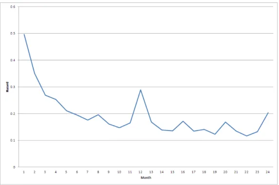
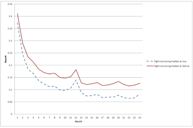
1. Uncensored price spells only group. For each price spells, a price change happens at the end. Therefore, all censored spells are excluded. The …gure 2-4 reports that during the …rst a few months, the hazard function is downward sloping. Then it becomes relatively ‡at, with signi…cant 12 month spike. This …nding is consistent with the previous …ndings in other countries, such as Alvarez et al.(2005) and Nakamura and Steinsson (2008). However, the reciprocal of sum of survival rates

$= 0:29, which is too much higher than the frequency of price change we directly calculated from whole sample. This indicates that the uncensored price spells scheme su¤er the loss of long price spells.

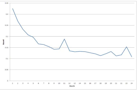
2. Left censored price spells only group. The reciprocal of sum of survivor rate $= 0:18. As Figure 2-5 shows, the shape of hazard function is similar to what we get from the normal price spell, though with smaller annual spikes. The biggest problem when we included the left censored price spell is that we do not really know when the price spells start. The statistical treatment of such spells induces more

(56)

Figure 2-4: Hazard function for normal price spells

di¢ culties than accounting for the sole right-censoring. However, the sample we have is made of thousands of spells for similar products in quite similar outlets -i.e. we have ma