Quantitative goals for monetary policy

WO R K I N G PA P E R S E R I E S

ISSN 1561081-0

N O 6 1 5 / A P R I L 2 0 0 6

QUANTITATIVE GOALS

FOR MONETARY POLICY

In 2006 all ECB publications will feature a motif taken from the €5 banknote.

W O R K I N G PA P E R S E R I E S

N O 6 1 5 / A P R I L 2 0 0 6

This paper can be downloaded without charge from http://www.ecb.int or from the Social Science Research Network electronic library at http://ssrn.com/abstract_id=891017

QUANTITATIVE GOALS

FOR MONETARY POLICY

by Antonio Fatás

,

Ilian Mihov

and Andrew K. Rose

1 Fatás is Professor of Economics, INSEAD, and CEPR Research Fellow. Mihov is Associate Professor of Economics, INSEAD and CEPR Research Fellow. Rose is Rocca Professor of International Business, NBER Research Associate and CEPR Research Fellow. Rose thanks INSEAD, the Reserve Bank of Australia, and the Monetary Authority of Singapore for hospitality while this paper was written. For INTERNATIONAL RESEARCH FORUM ON MONETARY POLICY

© European Central Bank, 2006 Address

Kaiserstrasse 29

60311 Frankfurt am Main, Germany Postal address

Postfach 16 03 19

60066 Frankfurt am Main, Germany Telephone +49 69 1344 0 Internet http://www.ecb.int Fax +49 69 1344 6000 Telex 411 144 ecb d All rights reserved.

Any reproduction, publication and reprint in the form of a different publication, whether printed or produced electronically, in whole or in part, is permitted only with the explicit written authorisation of the ECB or the author(s).

The views expressed in this paper do not necessarily reflect those of the European

International Research Forum on Monetary Policy: Third Conference

This paper was presented at the third conference of the International Research Forum on Monetary Policy which took place on May 20-21, 2005 at the ECB. The Forum is sponsored by the European Central Bank, the Board of Governors of the Federal Reserve System, the Center for German and European Studies at Georgetown University and the Center for Financial Studies at Goethe University. Its purpose is to encourage research on monetary policy issues that are relevant from a global perspective. It regularly organises conferences held alternately in the Euro Area and the United States. The conference organisers were Ignazio Angeloni, Matt Canzoneri, Dale Henderson, and Volker Wieland. The conference programme, including papers and discussions, can be found on the ECB’s web site (http://www.ecb.int/events/conferences/html/intforum3.en.html)

C O N T E N T S

Abstract 4

Non-technical summary 5

1. Introduction and motivation 7

2. Literature review 8

3. Methodology 14

3.a Benchmark model 15

3.b Data description 17

4. Empirics 21

4.a Benchmark results 21

4.b Sensitivity analysis 22 4.c Output volatility 28 5. Conclusions 30 References 32 Tables 35 Appendices 42 Figures 56

Abstract

We study empirically the macroeconomic effects of an explicit de jure quantitative goal for

monetary policy. Quantitative goals take three forms: exchange rates, money growth rates, and inflation targets. We analyze the effects on inflation of both having a quantitative target, and of hitting a declared target; we also consider effects on output volatility. Our empirical work uses an annual data set covering 42 countries between 1960 and 2000, and takes account of other determinants of inflation (such as fiscal policy, the business cycle, and openness to international trade), and the endogeneity of the monetary policy regime. We find that both having and hitting quantitative targets for monetary policy is systematically and robustly associated with lower inflation. The exact form of the monetary target matters somewhat (especially for the

sustainability of the monetary regime), but is less important than having some quantitative target. Successfully achieving a quantitative monetary goal is also associated with less volatile output.

Keywords: transparency; exchange; rate; money; growth; inflation; target; business cycle.

Non-technical summary

The economics profession has gradually moved to the view that transparency in monetary (and other) policies is desirable. For instance, the IMF believes that transparent policies are both more effective and enhance accountability. But while the theoretical advantages of transparency have been much analyzed, there is less in the way of empirical support. One objective of this paper is to help fill that gap.

We approach this problem empirically by using a panel of annual data covering over forty countries from 1960 through 2000. We identify “transparent” targets for monetary policy with “quantitative” targets. Quantitative targets are easily measured, allowing the monetary authority’s successes (or lack thereof) to be determined mechanistically. That is, quantitative targets are transparent since they can be assessed without (much) debatable personal judgment. However, we are not interested in just the effects of having a transparent policy, but also in the

effects of successful transparent policy. That is, we are interested in both the de jure monetary

regime, and the de facto success of a central bank in hitting its target (if one exists). Using

regression analysis, we find that in practice countries with transparent targets for monetary policy achieve lower inflation, holding other things constant. We also find that countries that hit their targets achieve lower inflation.

In practice, central banks have used three types of quantitative monetary targets, with varying degrees of success: exchange rates, money growth rates, and inflation targets. A number of economists in the past have analyzed the effects of one of these regimes. For instance, there is a large and growing literature on countries with inflation targets. There is an even larger

literature that compares the merits of fixed and floating exchange rate regimes. Rather than focusing on any one of these targets, we use all three. In part this is because we are interested in

estimating the effect of transparency in monetary policy, and transparency can take different forms. Indeed, when we compare the effects of different quantitative targets for monetary policy

(exchange rate/money growth/inflation) on inflationary outcomes, we find differences, but they

are small compared to the presence of any transparent target.

Still, we combine together different types of targets for monetary policy for a more important reason, best explained with an example. Fixed exchange rates are well-defined monetary policies, and are often compared with floating exchange rate regimes. But a float is not a well-defined monetary policy! Similarly, central banks that do not target inflation have to

do something else. By using data for all quantitative monetary regimes, we can reasonably

compare the merits of having a transparent monetary policy to the alternative, which we consider to be “opaque monetary objective(s).”

1. Introduction and Motivation

The economics profession has gradually moved to the view that transparency in monetary (and other) policies is desirable. For instance, the IMF believes that transparent policies are both more effective and enhance accountability. Accordingly, the Fund encourages countries “… to state clearly the role, responsibility and objectives of the central bank. The objectives of the

central bank should be clearly defined, publicly disclosed and written into law.”1 But while the

theoretical advantages of transparency have been much analyzed, there is less in the way of empirical support. One objective of this paper is to help fill that gap.

We approach this problem empirically by using a panel of annual data covering over forty countries from 1960 through 2000. We identify “transparent” targets for monetary policy with “quantitative” targets. Quantitative targets are easily measured, allowing the monetary authority’s successes (or lack thereof) to be determined mechanistically. That is, quantitative targets are transparent since they can be assessed without (much) debatable personal judgment. However, we are not interested only in the effects of transparent policy, but in the effects of

successful transparent policy; that is we are interested in both the de jure monetary regime, and

the de facto success of a central bank in hitting its target (if one exists). Using regression

analysis, we find that in practice countries with transparent targets for monetary policy achieve lower inflation, holding other things constant. We also find that countries that hit their targets achieve lower inflation.

In practice, central banks have used three types of quantitative monetary targets (with varying degrees of success): exchange rates, money growth rates, and inflation targets. A number of economists in the past have analyzed the effects of one of these regimes. For instance, there is a large and growing literature on countries with inflation targets. There is an

even larger literature that compares the merits of fixed and floating exchange rate regimes. Rather than focusing on any one of these targets, we use all three. In part this is because we are interested in estimating the effect of transparency in monetary policy, and transparency can take different forms. Indeed, when we compare the effects of different quantitative targets for

monetary policy (exchange rate/money growth/inflation) on inflationary outcomes, we find

differences, but they are small compared to the presence of any transparent target.

Still, we combine together different types of targets for monetary policy for a more important reason, which is best explained with an example. Fixed exchange rates are well-defined monetary policies, and are often compared with floating exchange rate regimes. But a float is not a well-defined monetary policy! Similarly, central banks that do not target inflation

have to do something else. By using data for all quantitative monetary regimes, we can

reasonably compare the merits of having a transparent monetary policy to the alternative, which we consider to be “opaque monetary objective(s).”

In section 2, we review the extensive literature of relevance; our methodology and data set are presented afterwards. The core of our paper is in section 4, which presents our results for inflation, along with sensitivity analysis. We then analyze the effects of quantitative targets on the short run/business cycle volatility of output. A brief conclusion closes.

2. Literature Review

Our work is related to a number of other classic problems in economics. One is the choice of monetary target. Different target have different degrees of transparency (as well as other attributes); accordingly, many scholars have addressed the question of whether central

banks should use the exchange rate, the money growth rate, the inflation rate, or something else.2 Most of this literature is concerned with exchange rate regimes. There is an enormous literature that compares the attributes of fixed and floating exchange rate regimes, both theoretically and empirically. Still, to repeat a standard but important criticism of this area, a fixed exchange rate is a well-defined monetary policy, but a floating exchange rate regime is not. If the monetary authorities are not pegging the exchange rate, they must be doing something else. Because of the recent increase in the adoption of inflation targets, we have seen a shift in the literature towards the study of inflation targeting regimes. Another related literature is that of the optimal degree of

transparency in monetary policy.3

There is also a literature that has focused on the role of domestic institutions in the conduct of monetary policy, most of which is centred on the effects of independence of central banks, and/or, more recently, on inflation targets. Although these areas of the literature are ultimately addressing the same issue (how monetary policy regimes affect macroeconomic outcomes), it is fair to say that, to a large extent, they have been developed separately. We now review some of the key papers in each of these strands of literature, summarizing their main insights.

Exchange Rate Regimes

The macroeconomic effect of the exchange rate regime is still an open question, one that is associated with many controversies in both the international and monetary economics

literatures. There is a broad literature that deals with the theoretical analysis on the costs and benefits of different exchange rate arrangements and there is a consensus on the main factors that

2 _{See e.g., Atkeson and Kehoe (2001) NBER WP 8681.}

shape these costs and benefits. However, there are still many disagreements on the relative empirical importance of these factors. As a result, when it comes to the best monetary policy regime for a given country, most of the predictions are inconclusive as they depend on a variety of assumptions that can only be validated empirically. Relative to the theoretical literature, there have been fewer papers that have taken these assumptions to a test or that, more generally, have empirically estimated the implications of monetary policy regimes.

One of the first papers to provide a comprehensive empirical study of the effects of different exchange rate regimes on macroeconomic outcomes is Baxter and Stockman (1989). Using a cross-section of countries with different exchange rate regime, they looked at the association between the exchange rate regime and variables such as output, consumption, trade flows, government consumption and the real exchange rate. Their conclusion was that the exchange rate regime did not matter for most of the macroeconomic variables, with the exception of the real exchange rate (that was more volatile under flexible exchange rate systems). Flood and Rose (1995) corroborate and extend this finding to other determinants of exchange rates.

Most of the studies that have followed Baxter and Stockman (1989) have had a narrower focus; they look mainly into the consequences on inflation and output volatility. Recent studies by Ghosh et al. (1997, 2002) and Levy-Yeyati and Sturzenegger (2001) provide detailed

analyses of the effects of exchange rate regimes on inflation. The approach is to look initially at the marginal effect of the exchange rate regime, after controlling for the effect of money growth. The hypothesis is that the exchange rate regime has a direct effect on the relationship between money and inflation, beyond any potential indirect effect through the conduct of monetary policy

(i.e. on money growth rates). There is evidence that inflation is lower under fixed rate regimes.4

Levy-Yeyati and Sturzenegger (2003) and Ghosh et al. (1997) study the effects on business cycle volatility and growth. Regarding business cycle volatility, their results are consistent: fixed exchange rate regimes are associated to greater output volatility. Regarding growth effects, the papers reach different conclusions. While Ghosh et al. (1997) do not find strong evidence in any direction Levy-Yeyati and Sturzenegger (2003) conclude that growth is higher for floaters.

Domestic Institutions

Even for countries where the discussion on exchange rate regimes is not important (in most cases because of the adoption of floating exchange rates), there has been an active recent debate on optimal monetary policy. The two key issues are typically whether the central bank should have goal-independence, and whether it should have an explicit inflation target.

Regarding the independence of central banks, the literature has focused on the observed negative correlation between inflation and central bank independence as documented in Alesina and Summers (1993), Cukierman (1992) or Grilli et al. (1991).

The other main features of monetary policy that have been studied in this literature are the effects of explicit targets and transparency. Initially the analysis was centred on money targets, but as countries moved away from these targets into inflation ones, the focus of the literature has moved accordingly. Because of the lack of a large number of observations, the literature tends to be descriptive, based on case studies rather than cross-country regressions. Mishkin (1999) and the books by Bernanke, Laubach, Mishkin and Posen (1999) and Loayza and Soto (2002) present good surveys and case studies of money and inflation targeting. Overall the

budget balance, a set of regional dummies and the exchange rate dummies. Once again long pegs are the only cases where there seems to be a significant negative effect on inflation, in this case through lower money growth.

evidence is mixed. There is evidence that inflation targets have helped countries reduce their inflation rates (Mishkin and Schmidt-Hebbel, 2002). On the other hand, Ball and Sheridan (2005) argue that this effect has been due to factors other than the monetary regime (while assuming that inflation reverts to a low mean).

Regimes

In all the literature reviewed above, two issues appear repeatedly: the characterization of monetary policy regimes (especially when it comes to exchange rate regimes) and the problem of endogeneity.

Classification of regimes: words or actions? When it comes to the classification of

exchange rate regimes, there are two possible approaches. The first is to look at the officially

declared de jure regime. The problem with this approach is that we often observe in practice that

countries sometimes peg their exchange rate without a clear de jure commitment (or intervene

frequently despite having declared a floating exchange rate, the “fear of floating” as defined by Calvo and Reinhart, 2000). As an alternative one can look at actions and classify regimes but looking at the actual behaviour of exchange rates (or the target set by monetary policy), i.e., the

de facto regime. This is the approach of Reinhart and Rogoff (2004) and Levy Yeyati and

Sturzenegger (2001, 2003). Their results show that looking at a de facto classification might

provide very different results. The distinction between words and actions also matters for other monetary policy targets such as money and inflation targets. For example, there is plenty of evidence that central banks that declared themselves to be money targetters were not behaving as such (see, for example, Bernanke and Mihov (1997) for the case of the Bundesbank).

Rather than attempt to resolve this issue on a conceptual level, we look at both the effects

of having a transparent de jure monetary regime, and whether or not it is hit de facto in practice.

Dealing with endogeneity. The interpretation of the existence of a correlation between

inflation (or output volatility) and the exchange rate regime is problematic because of

endogeneity. Is inflation lower because of the fixed exchange rate regime? Or are countries with low inflation (or more distaste of inflation) more likely to adopt fixed exchange rate regimes? The literature has dealt with the issue of endogeneity by using a set of instrumental variables

based on either economic or political arguments.5 Levy-Yeyati, Sturzenegger and Reggio (2002)

or von Hagen and Jizhong Zhou (2004) provide a comprehensive study of the endogeneity of exchange rate regimes. Frieden, Ghezzi and Stein (2000), within the context of Latin America, use a similar framework. Alesina and Wagner (2003) provide an analysis of how institutions affect decisions by countries to abandon fixed exchange rate regimes and to dissemble why such regimes are in place.

The arguments about what determines the choice of an exchange rate regime are based on theories that highlight the economic costs and benefits of the regimes, as well as the political institutional environment in which different regimes might be preferable. The economic variables are related to the optimum currency area debate. What makes a country a better candidate to adopt the currency of a different country? Openness, size, geographical

concentration of country’s trade, the type of shocks (volatility of terms of trade, volatility of other nominal versus real shocks), financial dollarization all matter to assess these costs and benefits and have been used as instrumental variables in the literature.

5 _{A separate but related issue is the need to control for variables other than the monetary policy regime in the}

determination of inflation. Romer (1993) or Lane (1997) are examples of papers that have studied how the determinants of the incentives of governments to inflate their economies.

The political arguments are more institutional, and concern the benefits of committing to a certain monetary policy. From a theoretical point of view, fragmentation of power (measured by e.g., the fraction of seats in congress held by government, years in office, or a Herfindahl index of political parties) or political instability shape the benefits and costs of commitment when it comes to monetary policy or the exchange rate regime. There is evidence that these variables matter (Frieden, Ghezzi and Stein (2000) or Edwards (1996)).

The issue of endogeneity has rarely been studied in the case of money or inflation targets. One of the few exceptions is Gerlach (1999) in the context of inflation targets. His results show that the adoption of inflation targets is more likely with low degree of central bank

independence, less openness, countries that export a low number of goods and among members of the EU.

3. Methodology

Our question is whether the establishment of a quantitative target for monetary policy

matters for inflation, ceteris paribus, and also whether hitting a target (if it exists) matters. We

can think of two ways to proceed. First, we could pursue case studies, as is done in much of the literature. This has a number of advantages. Precise details concerning monetary institutions, policy, and other factors can be used. The underlying economy changes little, so one can focus on monetary policy. It is difficult to measure monetary regimes perfectly; for instance some countries began dis-inflation programs without a contemporaneous switch in monetary regime (New Zealand in the late 1980s and Sweden in the mid 1990s come to mind). Still, the case study approach has a big disadvantage: one does not end up with estimates that are general. Accordingly, in this paper we seek to extend the literature by pursuing an econometric approach

that spans both long periods of time and a number of countries. The advantage of our approach is its generality, but it may come at the cost of precision. In particular, we are forced to restrict ourselves to variables that can be measured similarly for a large number of observations; we highlight these issues below.

3.a Benchmark model

Our benchmark model is the following:

Πit = β1DJTargetit + β2Successit

+ γ1Openit + γ2Budgetit + γ3BusCycleit + γ4GDPpcit + γ5 GDPit + εit

where i denotes a country, t denotes a year, and

• Π denotes the annual inflation rate in percentage points

• DJTargett is a dummy variable that is one if the country had a quantitative monetary policy

target during period t, and zero otherwise,

• γi is a set of nuisance coefficients,

• Success is a dummy variable that is one if the country hit its de jure quantitative target during

t, and zero otherwise,

• Open is trade (exports plus imports) as a percentage of GDP,

• Budget is the government budget surplus (+) or deficit (-), as a percentage of GDP,

• BusCycle is the difference between real GDP growth and average (country-specific) GDP

growth, measured in percentage points,

• GDPpc is the natural logarithm of real GDP per capita,

• GDP is the natural logarithm of real GDP, and

The two coefficients of interest to us are β1 and β2. The first coefficient is of greatest

interest; it represents the effect of having a formally declared de jure quantitative monetary target

on inflation, ceteris paribus. Also of interest to us is β2, which shows the effect on inflation of

successfully hitting a quantitative monetary target (if one exists) de facto.

The other regressors control for “nuisance” factors that affect inflation and might be correlated with the monetary policy regime, but are not of direct interest to us. Romer (1993) argues that more open economies have lower inflation because the costs of monetary expansion are high when the country has high trade-to-GDP ratio. More open economies might also opt for a fixed exchange rate relative to their trading partners as argued by the literature on the optimal

currency areas. This argument prompts us to include Open as a regressor. The budget balance

(Budget) can affect inflation by imposing requirements for money-financed deficits or through

aggregate demand. At the same time the success in hitting a monetary target can be affected by

fiscal policy outcomes. We also include the state of the business cycle (BusCycle) as a measure

of aggregate demand pressures on the price level and as a covariate that might be correlated with

the success of the monetary regime. GDP per capita (GDPpc) enters the regression to account

for the fact that rich countries have more sophisticated financial sectors, which implies higher opposition to inflation (as in Posen, 1995) and lower optimal inflation tax because of better-developed standard tax instruments. Posen’s argument also suggests that rich countries have low incentives to adopt an explicit target given that there is already pressure to achieve low inflation. Finally, the level of GDP is included to account for the market size. Since market size can affect productivity as in the models of Romer (1986) or Lucas (1988), a larger country may have lower

inflation ceteris paribus. On the correlation between country size and explicit targets, one might

Our benchmark regression is similar to those used by Levi-Yeyati and Sturzenegger (2001), and Ghosh et al. (2002). The theoretical motivation for their econometric specification is quite similar to ours, except that these studies focus only on the exchange rate regime. Campillo and Miron (1996) provide also a cross-sectional investigation of determinants of inflation and the regressors are almost identical to the ones we use, but they do not include any variable that captures the nature of the monetary regime.

We estimate the model with least squares, and use robust standard errors. Still, we are cognizant of a number of potential econometric pitfalls associated with this strategy (e.g., simultaneity). Accordingly, we do perform extensive sensitivity analysis to take into account a variety of different issues.

3.b Data Description

A data appendix describes in detail the sources and the list of variables used in our empirical analysis. Our annual data set spans 1960 through 2000, and includes all countries with 1960 GDP per capita of at least $1000 dollars in the Penn World Table database for which comprehensive data are available. There is significant variation in monetary policy practices both over time and across countries in the data set. Exchange rate pegs are more common in the 1960s, money targets disappear from many countries during the 1980s, inflation targeting only appears in the 90s. For most of our analysis we use annual frequency (given that we are not interested in high-frequency properties of the data), but we provide sensitivity analysis by replicating our results using five-year averages.

We use two variables to characterize the monetary policy regime: whether or not there

complementary to that of the previous literature. As mentioned in our literature review, previous papers have struggled with the issue of “words versus actions”. Central banks often claim to have adopted strict monetary policy targets, whether they are monetary aggregates, exchange rates, or inflation targets. In many cases these claims are not validated by their actions or the data. Some obvious examples of this behavior include: countries that intervene on foreign exchange markets extensively despite having a floating exchange rate policy; missed targets for

monetary aggregates; and missed inflation targets. Our strategy is to capture with our de jure

classification of monetary regimes the stated announcements of central banks, and then also to look separately at whether or not the target was hit in practice.

Establishing a de jure classification for exchange rate and inflation targets is not

conceptually complicated, though there is much debatable minutiae. In the case of targets for monetary aggregates, there are several cases where a judgment call needs to be made; many

central banks use monetary aggregates as reference indicators for their monetary policy without

formally targeting money growth. We try not to take this logic too far, because we are interested

in words (not actions) for our de jure classification. For example, the Bundesbank is classified

as having a target for money even though we know that in practice the commitment to the target was weaker than the Buba’s words.

There is one complication that we have to address before we proceed with the estimation of our benchmark model. Sometimes countries change their monetary regimes in mid-year. This presents a potential problem for our estimation because for the year when there is a change we will use data for the dependent variable and the controls that correspond to two regimes at the same time. Had we known the exact date of the regime change, we could remove that year.

Unfortunately we do not have this information for a good number of observations.6 Accordingly, we delete adjacent years with different regimes, so that each regime shift entails two dropped observations. The impact of a switch in monetary regime may be pronounced in the year when it takes effect, especially for countries that are engaged in a dis-inflation campaign, so this may

dilute our estimates.7 We feel most comfortable proceeding conservatively, and cannot see any

bias associated introduced by this convention.

Our de facto classification of monetary policy regimes provides a measure of whether or

not the announced targets were met. For simplicity, we classify monetary authorities as either hitting or missing their targets; that is we use a binary 0/1 variable to indicate success or failure of the monetary authorities in achieving their target. Future work might consider finer or continuous gradations of success, since central banks often have partial success in hitting

monetary targets.8

In the case of the exchange rate targets we make use of the Reinhart and Rogoff classification that characterizes exchange rate regimes by their actions (not their words). This has the advantage of covering a broad array of countries, and was not created by us (so that it is

objective).9 In the case of inflation and money targets we simply compare the outcome (inflation

or money growth) with the announced range for the target. Still, we face several difficulties in making this comparison. First, targets are sometimes expressed as a single number, while for

6 _{When we know the date of a regime shift, we follow the convention of dating it to the year when it was first in}

place for at least six months.

7 _{For instance, when Canada introduced money growth targeting in 1976, its inflation fell from 10.8% the year}

before to 7.5%. A more extreme example is the introduction of the Argentine convertibility; when it was introduced in 1991, inflation fell from over 2000% to around 170%.

8 _{It would be natural to pursue this angle through a loss function approach, though there could be problems if the}

monetary target is a range rather than a point.

9 _{Reinhart and Rogoff treat realignments from one fixed exchange rate to another as falling within a fixed exchange}

rate regime. This is debatable; on the one hand, the central bank has not achieved its monetary target, while on the other hand the monetary regime remains intact “in the large.” We return to this issue below when we consider IV estimation.

others a range is provided. When an explicit range is provided we simply assess whether or not the outcome is within the range. If there is no band around the announced target, we either consider the target as a maximum (by establishing a range from 0 to the announced value) or we build a range around the target. We consider the value as a maximum when the central bank is clearly trying to bring inflation down and establishes a series of decreasing targets for the years ahead. We add a range to the target when this is consistent with previous or future behavior of that central bank. For example, there are also instances where central banks switch from an explicit range to a single point. In those cases we add a band of around the announced target of

the same size as the band that was in place in previous years.10

The second difficulty associated with determining whether or not a target was hit is measuring the outcome. Money and inflation targets are established for a specific measure of inflation or a monetary aggregate. In some cases, the information about the precise measure being used is unavailable. In others, we know the variable used, but have not been able to find the data. As a result, we are missing some observations. In the case of inflation, we use the CPI as our measure of the price index. In the case of monetary aggregates, we normally use

information on both target and outcome that originate from the same source.11

The appendix also provides two figures with a comprehensive set of simple country-by-country time series plots of inflation; different monetary regimes are marked by different

symbols. During this period of time, lower inflation was typically better inflation, though not for all countries and period of time (e.g., Japan during the 1990s which probably experienced

10 _{In the very few cases where we cannot find information or a historical reference to establish a band, we use the}

excessively low inflation). Thus our methodology does not deliver a message about welfare, and it would be inappropriate for a sample where inflation was typically low.

Perhaps a more effective way to present the data graphically is through an “event study.” Figure 3 is a set of event studies that look at inflation around the dates of changes in monetary regime. The top left-hand diagram examines inflation in the three years before, during (marked

by the vertical line), and after entry; it considers entry into de jure regimes of any sort. The

middle line (with circles) shows the mean level of inflation, while the two other lines show a confidence interval of plus and minus two standard deviations. The diagram in the top

right-hand corner is the analogue showing exits from de jure regimes, while the diagrams below are

analogues that exclude the high-inflation countries. While none of the event studies is overwhelmingly persuasive, each of them provides a message consistent with the results we verify more rigorously below. In particular, the entry intro a monetary regime with a quantitative target coincides with a reduction in inflation, while exits from such regimes are associated with increases.

4. Empirics

4.a Benchmark Results

OLS estimation of our model results in the benchmark estimates presented in Table 1.

The coefficient of greatest interest to us is β1, the effect on inflation of a country’s having a

quantitative target for monetary policy of any type (whether an inflation target, a money growth target, or an exchange rate target). The effect is both economically and statistically significant;

the existence of a de jure target is estimated to lower annual inflation by about sixteen

zero at all conventional significance levels). This effect is enhanced if the quantitative target is actually hit. A monetary target that is successfully achieved reduces inflation by another five percentage points, a result that is again highly statistically and economically significant.

Our basic framework is perturbed in three ways in Table 1. First, we drop the dummy variable for successful implementation of a quantitative monetary target. Second and

symmetrically, we also drop the dummy representing the existence of a quantitative target. Each of the coefficients remains economically and statistically significant if the other is set to zero.

Finally, we drop all the conditioning variables (that is, we set γ1=γ2=…=γ5=0).

At first blush it seems that countries with transparent (quantitative) de jure monetary

targets experience lower inflation. Actually hitting the target lowers inflation further. While the preliminary findings are positive, caveats certainly exist. For one thing, the model fits the data poorly. While many of the auxiliary regressors are correctly signed (more open economies have lower inflation; tight fiscal policy lowers inflation; richer economies have lower inflation), some are not (observations with higher-than-average growth display lower inflation). Furthermore, a number of potentially important omitted variables and econometric complications come to mind quickly. Accordingly, we now engage in sensitivity analysis.

4.b Sensitivity Analysis

Table 2 checks the sensitivity of the results with respect to the precise sample used for estimation. First we drop observations before 1975. Next we drop all observations where the (country x year) observation is for a country with real GDP per capita below $5,000. Another perturbation restricts our attention to long-time OECD members (those that entered before 1975).

Next we drop outlier observations.12 Our last two changes are to add in Argentina and Brazil, two high inflation countries, and then to drop all high inflation countries, defined as a country which experienced inflation exceeding 100% annually at any point in our sample (Chile, Israel,

Mexico, Turkey and Uruguay). It is striking that our key coefficient of interest – β1 – remains

economically large and statistically significant in all of these perturbations. (The size of the effect of course varies with the sample; excluding high-inflation countries reduces considerably

the potential and actual influence of a quantitative monetary target.) Further, β2 is also

significantly negative (in both the economic and statistical senses) in all cases except when

Argentina and Brazil are included in the sample.13

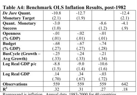
Do our results depend on regime switches associated with major oil price shocks? No. In an appendix we tabulate the analogues to Tables 1 and 2, computed only with data after 1982. These show quite similar results to our benchmark results. Appendix Table A6 tabulates

estimates of the key coefficients computed from the four different decades of data. Again, our key coefficients remain negative (and mostly significant at standard confidence levels) with the

exception of the 1960s de jure coefficient, which is insignificantly positive. It seems that

restricting ourselves to data after the second OPEC oil price shock does not change our results

substantively.14

In Table 3 we check the robustness of our results with respect to unobserved country- and time-specific factors. We do this by adding successively: a) country-specific intercepts, b) year-specific intercepts, and c) and year-year-specific intercepts simultaneously. Using

12 _{The latter are defined as observations with a residual estimated to lie more than 1.5 standard deviations from the}

mean of zero.

13 _{We have also dropped the countries with maximal inflation exceeding 38.2% (which corresponds to the 75}th

percentile of our sample), and countries with average inflation exceeding 13% (which again corresponds to the 75th

percentile of our sample). In both cases, the coefficients on both de jure quantitative regimes and the success in

hitting the target remain negative, though only the latter coefficients are significantly different from zero.

14 _{We also note that there is a poor overlap between departures from quantitative monetary regimes and major oil}

specific fixed effects is an important check, since it means that the estimation relies only on within-country variation in inflation and monetary regimes over time. Using year-specific fixed effects because it accounts for any global factors such as oil prices global inflation and the global business cycle. Another column of the table adds dynamics to the perturbation with both sets of fixed effects by modeling the error term as an AR(1) disturbance rather than serially

uncorrelated. Finally, we use the one-year lead of inflation in the last column on the right, since

inflation responds to policy with a lag.15 Again, our key coefficient remains negative and

significant throughout (though adding country effects eliminates the significance of the effect of achieving a monetary target).

Table 4 explores whether the three types of quantitative monetary policy targets – inflation, money growth, and exchange rate – have similar effects on inflation. When the three different regimes are allowed to take on different coefficients, the inflation-targeting regime seems to have more of a dampening effect on inflation than the (similar) effects of either

exchange rate or money growth targets. The differences between the three targets are significant at conventional confidence levels. The effect of a successfully hit monetary target on inflation also varies by the type of target; surprisingly, the effect of successfully hitting an inflation target

has a positive coefficient.16 _{Still, the most important differences between different types of}

monetary regimes may be not in their outcomes, but their sustainability. Many countries have abandoned both exchange rate and money growth targets; none has (yet) abandoned an inflation target. Our analysis does not capture these differences, and this would be an interesting area for future research.

15 _{Using a lead of inflation also helps to reduce problems with endogeneity; more on that below.}

16 _{A closer inspection of the data reveals that several countries have indeed missed the target by having inflation}

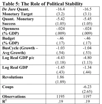
Table 5 shows that the effects of political instability on inflation are of negligible importance using revolutions and coups (the variables used by Campillo and Miron, 1996). While coups are associated with a drop in inflation, our key coefficients are little affected.

Table 6 uses instrumental variables estimation to account for possible simultaneity in the

equation.17 We are particularly concerned with the possibility that high inflation induces the

authorities to introduce or use quantitative targets. There is also the possibility that a low inflation environment may encourage the authorities to lock in stability with a transparent monetary policy.

As instrumental variables for both our de jure monetary dummy, and the dummy variable

for de facto success in hitting this target, we use three political variables and two variables

capturing social characteristics. They are: a) political constraints (used by Henisz, (2000)); b) a dummy for (country x year) observations with a presidential electoral system (taken from Persson-Tabellini, 2001); c) a comparable dummy for observations with majoritarian electoral systems (again taken from Persson-Tabellini, 2001); d) the percentage of males over 25 years old with completed primary education; and e) the percentage of males over 25 years with completed secondary education. We use these variables for a number of reasons. The presence of political constraints in the country reveals an overall preference for rules. In addition, countries with more political constraints have more disciplined fiscal policy. With more discipline on the fiscal side it is more likely that that a monetary regime is sustainable. A somewhat different argument is that if political constraints restrict fiscal policy, then society might prefer to leave monetary policy unconstrained and assign to it a bigger role in smoothing business cycle fluctuations. The nature of the political system (presidential vs. parliamentary) affects regime choice in a similar

17 _{Measurement error is also a potential issue, especially for de jure monetary performance; as we note above, there}

way. Presidential regimes are often characterized by better separation of powers than

parliamentary ones, because the president cannot be subjected to a no-confidence vote by the parliament (except under rare circumstances of impeachment). The executive in a parliamentary system, on the other hand, can be more easily removed. The separation of powers in a

presidential system again makes fiscal policy rather constrained, which boosts the case for having flexible monetary policy. The electoral system matters because countries with

majoritarian systems are associated with stronger governments relative to those with proportional representation. Proportional systems often lead to the need for coalitions to form a government; Levy-Yeyati, Sturzenegger and Reggio (2002) argue coalition governments are more prone to be influenced by special interests. To avoid a situation where special interests affect monetary policy, the society might opt for a regime with an explicit target. Hence majoritarian systems should be linked with a more flexible regime. Finally the two education variables are used since more educated societies may insist on having institutions for low inflation, while education has no direct effect on inflation.

We provide four different perturbations of our IV results: benchmark; with country-fixed effects; with year intercepts; and with both. The standard errors for the coefficients of interest are considerably higher, indicating that the first-stage regressions do not fit well. That is, our instrumental variables do not work particularly well. This is even more obvious from the

dramatic increase in the size of the effects; the IV estimates of β1 are approximately three times

the magnitude of the OLS estimates. Once we control for unobserved country fixed effects, the coefficient on monetary success in hitting a quantitative target becomes positive and significant.

It is difficult to provide a reasonable interpretation of this reversal. The effect of de jure regime

as instrumental variables the lags of the de jure regime and de facto monetary success.18 These

instruments help with addressing issues of omitted variables (e.g. a beneficial supply shock that leads to lower inflation and also helps the central bank hit the target). The results are highly significant and consistent with the findings of our benchmark model.

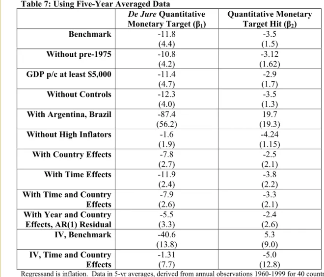
Our final set of experiments moves away from the annual domain to consider data averaged over mutually exclusive and jointly exhaustive five-year intervals between 1960 and 1999 (1960-64, 1965-69, and so forth). These are contained in Table 7, which tabulates our key coefficients estimated twelve different ways. For convenience, the auxiliary regressors

(openness, the budget, and so forth) are included in the regressions but not explicitly tabulated. The benchmark equation is presented in the top row. The other eleven perturbations we consider include: a) dropping observations before 1975; b) dropping all (time period x country)

observations with real GDP per capita below $5,000; c) dropping all controls (i.e., setting

γ1=γ2=…=γ5=0); d) adding Argentina and Brazil; e) dropping our five high inflation countries

(Chile, Israel, Mexico, Turkey and Uruguay); f) adding country intercepts; g) adding time-period effects; h) adding both country- and time-period fixed effects; i) adding an AR(1) residual to the country- and time-period intercepts; j) using IV on the benchmark equation; and k) using IV with

country and time-period intercepts. Our key coefficient, β1, remains negative, economically

large and statistically significant except when we exclude our high inflation countries and when we estimate the model by IV with time and country effects. Also when we include AR(1) errors into panel estimation the significance drops to about 10% level. This is ground for some caution, but not perhaps too much. Smoothing the data and excluding countries that have ever

18 _{This effectively deals with supply shocks that affect both inflation and the probability of}

de facto monetary

experienced high inflation may simply reduce the variation in inflation too much to allow the

effects of a quantitative target to be detectable.19

4.c Output Volatility

We now briefly present results on output volatility, which we investigate for two reasons. Many central banks (such as “flexible” inflation-targeters) care about stabilizing the output gap. We are also interested to see if the effects of transparent monetary regimes that we uncovered above come at the expense of increased output volatility.

Our benchmark model for the volatility regression is analogous to that for inflation:

σit = β1DJTargetit + β2Successit + γ1Openit + γ2Budgetit + γ3GDPpcit + γ4 GDPit + εit

where i denotes a country, t denotes a 5-year period, and

• σ denotes output volatility (defined carefully below), and

• other variables are as defined above.

For output volatility, we initially use the five-year average absolute deviation of output growth from mean growth (calculated from annual data). That is, we first compute the country-specific mean growth rate using the entire span of annual data, which we denote as

it t

i T GDP

GDP ≡ Σ ∆

∆ (1/ ) , then compute our regressand as σ_it ≡(1/5)Σ_τ |∆GDP_it −∆GDP_i| for

non-overlapping, mutually exclusive five-year periods, where GDP denotes the natural logarithm

of GDP.20

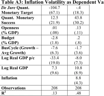
19 _{We have also searched without success for an effect of quantitative regimes on inflation}

volatility. Our results are

We start directly with five-year averages in order to provide a better estimate of business

cycle volatility. The coefficients of interest again are β1 and β2. The benchmark results for the

volatility equation are reported in Table 8. From the first column we conclude, that the

coefficients on both de jure and de facto regimes are not statistically significant at the 5% level

of significance. This implies that having an explicit target does not affect output volatility – that is, average absolute deviation of output growth from its mean. If the target is successfully achieved, however, then the volatility is reduced by about half of a percentage point. This result should not be over-interpreted as it is significant only at the 10% level.

The rest of Table 8 reports several sensitivity checks. In column 2 we drop the dummy

for “Success in achieving the target” and in column 3 we drop the de jure variable. In both cases

the estimates of the regime remain insignificant. Adding a lag of our volatility measure does not change the main conclusion that explicit targets do not affect significantly volatility of output.

In Table 9 we explore the sensitivity of these results in several dimensions. We start by including Argentina and Brazil in column (1) and by removing all of the high inflators in column (2). Again, hitting the target has a negative effect on volatility but statistically this result is significant at the 10% level at best. Adding unobserved time effects increases the significance of the success variable, but overall we find that there is little evidence to support any claim on the effect of policy regimes on output volatility.

Table 10 dis-aggregates the effects of monetary regimes on output volatility into those due to inflation, money growth, and exchange rate targets. There are no significant results that one can interpret here. Table 11 pursues instrumental variable estimation so as to account for endogeneity. When we use our political and education variables as instrumental variables, and

the scope of our project. Still, we see no reason why other de-trending techniques could not be used, such as those proposed by Hodrick and Prescott or Baxter and King. Constructing the output gap would also enable the sacrifice ratio to be compared across monetary regimes, which seems a worthwhile objective.

also when we add lagged regimes, the effects of de jure and de facto regimes remain statistically

insignificant, which could be again a signal that these are poor instruments or that volatility is indeed unrelated to the monetary policy regime. Finally, in Table 12 we provide analogues to OLS and IV estimation of our default model, but measuring output volatility in three different

ways: a) the average absolute value of the deviation of real GDP from HP-filtered real GDP (in

logs), b) the average absolute value of deviation of output growth from a ten-year average growth rate, or c) the standard deviation of output growth computed over (mutually exclusive)

decades of annual data.21 The estimates of having a de jure quantitative monetary target are

insignificant, but the estimates for successfully hitting this target are typically but not overwhelmingly statistically significant.

The conclusion from the volatility regressions is that, at a minimum, having an explicit monetary target does not increase the volatility of the economy. On the contrary, our evidence suggests that the coefficients on successfully hitting a target are negatively and significantly (in the economic sense) associated with lower volatility. Under several perturbations of our model these coefficients are statistically significant at the 10% level.

5. Conclusions

In this paper we investigate the effect of quantitative targets for monetary policy on inflation and business cycle volatility. We combine data for three types of targets for monetary policy (exchange rate targets, money growth targets, and inflation targets), so as to be able to compare the effects of both having and hitting transparent objectives for monetary policy against the alternative of having unclear or qualitative goals. Using a panel of macroeconomic data

target for the monetary authority tends to lower inflation and smooth business cycles; hitting that

target de facto has further positive effects. These effects are economically large, typically

statistically significant and reasonably insensitive to perturbations in our econometric

methodology. Differences in the exact form of the monetary regime have more minor effects on

actual inflation than having some quantitative target, though some monetary regimes seem more

easily sustainable than others.

During the past decade, there has been much emphasis placed on the importance of transparent goals for monetary authorities; the current consensus is that central banks should independently pursue well-defined goals in a transparent fashion. Our results lead us to conclude that this emphasis seems justified.

References:

Agenor, Pierre-Richard (2002), “Monetary Policy under Flexible Exchange Rates: An

Introduction to Inflation Targeting”, in Norman Loayza and Raimundo Soto (eds.) Inflation

Targeting: Design, Performance, Challenges, Central Bank of Chile.

Alesina, Alberto and Lawrence Summers (1993), “Central Bank Independence and

Macroeconomic Performance: Some Comparative Evidence,” Journal of Money, Credit and

Banking, 25:151- 62.

Alesina, Alberto and Alexander Wagner (2003), “Choosing and Reneging on Exchange Rate Regimes,” Harvard Institute of Economic Research Discussion paper no. 2008.

Atkeson, Andrew and Patrick J. Kehoe (2001), “The Advantage of Transparent Instruments of Monetary Policy,” NBER Working Paper no. 8681, December.

Ball, Laurence and Niamh Sheridan (2005), “Does Inflation Targeting Matter?” in Ben

Bernanke and Michael Woodford (eds.) The Inflation-Targeting Debate, Chicago, University

Press.

Baxter, Marianne and Alan Stockman (1989), “Business Cycles and the Exchange Rate System: Some International Evidence,” Journal of Monetary Economics 23, 377-400.

Bernanke, Ben, Thomas Laubach, Frederic Mishkin and Adam Posen (1999), Inflation

Targeting. Princeton, NJ: Princeton University Press.

Bernanke, Ben and Ilian Mihov (1997), “What Does the Bundesbank Target?” European Economic Review 41.

Calvo, Guillermo and Carmen Reinhart (2002), “Fear of Floating,” Quarterly Journal of Economics 117, 379-408.

Campillo, Marta and Jeffrey Miron (1997), “Why Does Inflation Differ Across Countries?” in

C. Romer and D. Romer (eds.) Reducing Inflation: Motivation and Strategy, Chicago: University

of Chicago Press.

Cottarelli, Carlo and Curzio Giannini (1997), “Credibility Without Rules? Monetary Frameworks in the Post-Breton Woods Era”, IMF Occasional Paper No. 154.

Cukierman, Alex and Allan Meltzer (1986), “A Theory of Ambiguity, Credibility, and Inflation

under Discretion and Asymmetric Information,” Econometrica 54, 1099-1128.

Cukierman, Alex (1992), Central Bank Strategy, Credibility and Independence: Theory and Evidence. MIT Press, Cambridge.

Edwards, Sebastian (1996), “The Determinants of the Choice Between Fixed and Flexible Exchange Rate Regimes,” NBER Working Paper No. 5756.

Faust, Jon and Lars Svensson (2002), “The Equilibrium Degree of Transparency and Control in

Monetary Policy,” Journal Of Money Credit And Banking, May.

Flood, Robert P. and Andrew K. Rose (1995) “Fixing Exchange Rates: A Virtual Quest for

Fundamentals” The Journal of Monetary Economics 36-1, 3-37.

Frankel, Jeffrey and David Romer (1999) “Does Trade Cause Growth?” American Economic Review, vol. 89 June.

Frieden, Jeffry, Piero Ghezzi and Ernesto Stein (2000), “Politics and Exchange Rates: A Cross-Country Approach to Latin America,” Inter-American Development Bank Working paper no. R-421.

Gerlach, Stephen (1999), “Who Targets Inflation Explicitly?” European Economic Review 43, 1257 – 1277.

Ghosh, Atish, Anne-Marie Gulde, Jonathan Ostry, and Holger Wolf (1997), “Does the Nominal Exchange Rate Regime Matter,” NBER Working Paper no. 5874.

Ghosh, Atish, Anne-Marie Gulde, and Holger Wolf (2002), Exchange Rate Regimes, Cambridge, MA: MIT Press.

Grilli, Vittorio, Donato Masciandaro and Guido Tabellini (1991), “Political and Monetary

Institutions and Public Financial Policies in the Industrial Countries”, Economic Policy, 341-302.

Henisz, Witold J. (2000), “The Institutional Environment for Economic Growth,” Economics

and Politics 12(1).

Lane Philip. (1997) ``Inflation in Open Economies,'' Journal of International Economics, 42,

May 1997, No.3/4, 327-346.

Levi-Yeyati, Eduardo and Federico Sturzenegger (2001), “Exchange Rate Regimes and

Economic Performance” IMF Staff Papers 47, 62-98..

Levi-Yeyati, Eduardo and Federico Sturzenegger (2003), “To Float or to Fix: Evidence on the

Impact of Exchange Rate Regimes on Growth”, American Economic Review 93(4).

Levi-Yeyati, Eduardo, Federico Sturzenegger, and Reggio (2002), “On the Endogeneity of Exchange Rate Regimes,” manuscript.

Loyaza and Soto (2002) (eds.), Inflation Targeting: Design, Performance, Challenges, Central

Lucas, Robert (1988), “On the Mechanics of Economic Development,” Journal of Monetary Economics 22, 3-42.

Mishkin, Frederic S. (1999), “International Experiences with Different Monetary Policy Regimes,” NBER Working Paper No. 7044.

Mishkin, Frederic S. and Schmidt-Hebbel Klaus (2003), “A decade of Inflation Targeting in the World: What Do We Know and What Do We Need to Know? in Norman Loayza and Raimundo

Soto (eds.) Inflation Targeting: Design, Performance, Challenges, Central Bank of Chile.

Persson, Torsten and Guido Tabellini (2001), “Political Institutions and Policy Outcomes: What are the Stylized Facts?” CEPR Discussion Paper No 2872.

Posen, Adam (1995), “Declarations Are Not Enough: Financial Sector Sources of Central Bank Independence,” in B. Bernanke and J. Rotemberg (eds.), NBER Macroeconomics Annual 10, Cambridge, MA: MIT Press, 253-274.

Reinhart, Carmen and Kenneth Rogoff (2004), “A Modern History of Exchange Rate

Arrangements: A Reinterpretation,” Quarterly Journal of Economics 119(1), pp. 1-48.

Romer, David (1993), “Openness and Inflation: Theory and Evidence,” Quarterly Journal of Economics 108, 869-903.

Romer, Paul (1986), “Increasing Returns and Long Run Growth," Journal of Political Economy

94, pp.1002-37

Siklos, Pierre L. (1999), “Inflation-Target Design: Changing Inflation Performance and

Persistence in Industrial Countries”, Federal Reserve Bank of St. Louis Review, March/April.

Sterne, Gabriel (2002), “Inflation Targets in the Global Context” in Norman Loayza and

Raimundo Soto (eds.) Inflation Targeting: Design, Performance, Challenges, Central Bank of

Chile.

von Hagen, Jurgen and Jizhong Zhou (2004), “The Choice of Exchange Rate Regime in Developing Countries: A Multinational Panel Analysis”, CEPR Discussion Paper, No. 4227.

Table 1: Benchmark OLS Inflation Results De Jure Quant. Monetary Target -16.5 (3.16) -20.8 (3.02) -16.8 (3.07) Quant. Monetary Success -5.52 (1.05) -14.8 (1.79) -4.88 (.90) Openness (% GDP) -.024 (.009) -.027 (.009) -.022 (.008) Budget (% GDP) -.46 (.17) -.49 (.17) -.46 (.18) BusCycle (Growth – Avg Growth) -1.01 (.53) -1.08 (.52) -1.00 (.54) Log Real GDP p/c -4.63 (1.10) -4.54 (1.11) -5.83 (1.27) Log Real GDP -1.31 (.44) -0.98 (.42) -1.53 (.46) Observations 1200 1340 1200 1408 R2 _{.19 .19 .16 .13}

Regressand is inflation. Annual data, 1960-2000 for 40 countries.

OLS with robust standard errors in parentheses. Intercepts included but not tabulated.

Table 2: Sample Sensitivity

Without pre-1975 GDP p/c at least $5,000 OECD Only Without outliers With Argentina, Brazil Without High Inflators De Jure Quant. Monetary Target -15.1 (2.6) -12.1 (2.24) -5.8 (1.8) -13.2 (2.14) -77.2 (21.2) -3.11 (.98) Quant. Monetary Success -4.14 (.99) -4.88 (1.02) -4.6 (.67) -5.69 (1.01) 11.2 (6.78) -3.57 (.53) Openness (% GDP) -.017 (.009) -.013 (.008) .030 (.014) -.019 (.007) -.037 (.04) -.015 (.004) Budget (% GDP) -.61 (.25) (.17) -.65 (.06) -.26 (.15) -.52 -1.27 (.99) (.04) -.13 BusCycle (Growth – Avg. Growth) -.99 (.75) -.53 (.20) -.82 (.27) -.45 (.18) -5.69 (3.31) -.45 (.14) Log Real GDP p/c -7.29 (1.52) -7.17 (1.33) -13.2 (2.0) -3.61 (.82) -30.4 (9.73) -2.17 (.42) Log Real GDP -.97 (.56) -1.11 (.50) (.37) .52 -1.16 (.42) (5.09) 12.3 (.18) -.74 Observations 817 989 699 1198 1232 1067 R2 _{.25 .31 .40 .27 .08 .24}

Regressand is inflation. Annual data, 1960-2000 for 40 countries.

OLS with robust standard errors in parentheses. Intercepts included but not tabulated. High Inflation countries are: Chile, Israel, Mexico, Turkey, and Uruguay.

Table 3: Robustness Checks Country Fixed Effects Year Fixed Effects Country, Year Effects Country, Year Effects Lead of Inflation De Jure Quant. Monetary Target -12.7 (2.5) -16.2 (2.2) -12.6 (2.5) -15.8 (3.5) -13.5 (3.0) Quant. Monetary Success -2.4 (2.1) -6.8 (2.0) -3.2 (2.1) .97 (1.85) -6.8 (1.3) Openness (% GDP) .16 (.04) (.014) -.025 (.04) .12 (.06) .07 (.01) -.02 Budget (% GDP) -.55 (.15) -.29 (.14) -.41 (.16) -.12 (.17) -.82 (.31) BusCycle (Growth – Avg Growth) -1.26 (.20) -.93 (.23) -1.19 (.21) -.41 (.13) -.38 (.32) Log Real GDP p/c -17.1 (7.5) -3.74 (1.33) -21.6 (7.4) 5.38 (16.8) -3.6 (1.0) Log Real GDP 3.1 (5.4) -1.22 (.57) 13.8 (6.4) -24.1 (13.0) -1.49 (.49) AR(1) Coefficient .87 Observations 1200 1200 1200 1161 1203 R2 _{.09 .19 .06 .01 .20}

Regressand is inflation. Annual data, 1960-2000 for 40 countries.

OLS with robust standard errors in parentheses. Intercepts included but not tabulated.

Table 4: Dis-Aggregating Monetary Regimes

De Jure Inflation Target -20.2 (2.5) -13.2 (1.83) Inflation Target Success 4.1 (1.9) De Jure Money Growth Target -11.2 (2.7) -7.6 (1.9)

Money Growth Target Success

-2.43 (3.23)

De Jure Exchange Rate

Target

-10.9 (4.0)

-16.7 (2.3)

Exchange Rate Target Success -10.2 (2.7) Openness (% GDP) -.021 (.009) -.027 (.009) Budget (% GDP) -.47 (.19) -.51 (.18) BusCycle (Growth – Avg Growth) -1.05 (.58) -1.08 (.54) Log Real GDP p/c -4.59 (1.26) -4.89 (1.19) Log Real GDP -1.11 (.51) -1.09 (.47) Observations 1023 1200 R2 _{.18 .17}

Regressand is inflation. Annual data, 1960-2000 for 40 countries.

Table 5: The Role of Political Stability De Jure Quant. Monetary Target -16.4 (3.2) -16.5 (3.1) Quant. Monetary Success -5.42 (1.05) -5.45 (1.05) Openness (% GDP) -.024 (.009) -.024 (.009) Budget (% GDP) -.46 (.17) -.46 (.17) BusCycle (Growth – Avg Growth) -1.03 (.54) -1.04 (.53) Log Real GDP p/c -4.43 (1.18) -4.80 (1.13) Log Real GDP -1.45 (.43) -1.34 (.44) Revolutions 1.86 (1.89) Coups -6.23 (2.65) Observations 1195 1197 R2 _{.19 .19}

Regressand is inflation. Annual data, 1960-2000 for 40 countries unless noted. OLS with robust standard errors in parentheses. Intercepts included but not tabulated.

Table 6: Instrumental Variable Results

Instrumental variables

Political Political and lagged regime Bench-mark Country Fixed Effects Year Fixed Effects Country, Year Effects Bench-mark Country Fixed Effects Year Fixed Effects Country, Year Effects De Jure Quant. Monetary Target -41.2 (16.9) (11.3) -33.4 (16.3) -34.6 (11.8) -29.4 -13.6 (3.2) -11.2 (2.9) -12.9 (2.6) -10.5 (2.9) Quant. Monetary Success -1.31 (11.2) 29.1 (12.3) -13.5 (10.2) 33.8 (19.8) -9.3 (1.7) -5.6 (3.1) -11.7 (2.6) -7.0 (3.2) Openness (% GDP) -.02 (.009) .14 (.06) .002 (.02) .10 (.06) -.022 (.008) .17 (.05) -.019 (.014) .13 (.05) Budget (% GDP) -.393 (.161) -.80 (.21) -.20 (.16) -.54 (.21) -.47 (.17) -.51 (.16) -.31 (.14) -.40 (.16) BusCycle (Growth – Avg Growth) -.86 (.53) -1.56 (.25) (.26) -.95 -1.47 (.27) (.55) -.99 -1.29 (.21) (.24) -.96 -1.23 (.22) Log Real GDP p/c -2.64 (2.11) -35.7 (15.5) -.41 (2.11) -49.7 (20.2) -5.29 (1.17) -15.7 (8.2) -4.15 (1.38) -21.6 (8.2) Log Real GDP -1.97 (0.74) 22.6 (13.6) -2.18 (.74) 32.9 (15.5) -1.78 (.49) .46 (6.2) -1.67 (.60) 13.0 (7.0) Observations 1149 1149 1149 1149 1149 1149 1149 1149 R2 _{0.09 .01 .17 .01 .20 .09 .19 .06}

Regressand is inflation. Annual data, 1960-2000 for 40 countries.

IV with robust standard errors in parentheses. Intercepts included but not tabulated.

Political instrumental variables for de jure quantitative monetary target and quantitative monetary success are: a)

political constraints (Henisz); b) Presidential Electoral System (Persson-Tabellini); c) Majoritarian electoral system (Persson-Tabellini); d) Percentage of males over 25 years old with primary education (Barro-Lee); and e) Percentage of males over 25 years old with secondary education (Barro-Lee);

Table 7: Using Five-Year Averaged Data De Jure Quantitative Monetary Target (β1) Quantitative Monetary Target Hit (β2) Benchmark -11.8 (4.4) -3.5 (1.5) Without pre-1975 -10.8 (4.2) -3.12 (1.62) GDP p/c at least $5,000 -11.4 (4.7) -2.9 (1.7) Without Controls -12.3 (4.0) -3.5 (1.3)

With Argentina, Brazil -87.4

(56.2)

19.7 (19.3)

Without High Inflators -1.6

(1.9)

-4.24 (1.15)

With Country Effects -7.8

(2.7)

-2.5 (2.1)

With Time Effects -11.9

(2.4)

-3.8 (2.2)

With Time and Country Effects

-7.9 (2.6)

-3.3 (2.1)

With Year and Country Effects, AR(1) Residual

-5.5 (3.3) -2.4 (2.6) IV, Benchmark -40.6 (13.8) 5.3 (9.0)

IV, Time and Country Effects

-1.31 (7.7)

-5.0 (12.8)

Regressand is inflation. Data in 5-yr averages, derived from annual observations 1960-1999 for 40 countries. Controls added but not recorded: openness; budget; business cycle growth deviation from mean; and logs of real GDP and real GDP per capita.

OLS with robust standard errors in parentheses. Intercepts included but not tabulated. High Inflation countries are: Chile, Israel, Mexico, Turkey, and Uruguay.

Instrumental variables for de jure quantitative monetary target and quantitative monetary success the following

political variables: a) political constraints (Henisz); b) Presidential Electoral System (Persson-Tabellini); and c) Majoritarian electoral system (Persson-Tabellini). d) Percentage of males over 25 years old with primary education (Barro-Lee); and e) Percentage of males over 25 years old with secondary education (Barro-Lee);