Hossein Taheri1 Aryan Mokhtari2 Hamed Hassani3 Ramtin Pedarsani1
Abstract
We consider a decentralized stochastic learning problem where data points are distributed among computing nodes communicating over a directed graph. As the model size gets large, decentral-ized learning faces a major bottleneck that is the heavy communication load due to each node transmitting large messages (model updates) to its neighbors. To tackle this bottleneck, we propose the quantized decentralized stochastic learning algorithm over directed graphs that is based on the push-sum algorithm in decentralized consen-sus optimization. We prove that our algorithm achieves the same convergence rates of the decen-tralized stochastic learning algorithm with exact-communication for both convex and non-convex losses. Numerical evaluations corroborate our main theoretical results and illustrate significant speed-up compared to the exact-communication methods.
1. Introduction
In modern machine learning applications we typically con-front solving optimization problems with massive data sets which demands utilizing multiple computing agents to ac-celerate convergence. Furthermore, in some applications each processing agent has its own local data set. How-ever, communicating data among different workers is often impractical from multiple aspects such as privacy and band-width utilization. In such settings, computing nodes rely on their own data to run (stochastic) gradient descent algorithm while exchanging parameters with other workers in each iteration to ensure converging to the optimal solution of the
1
Department of Electrical and Computer Engineering, Uni-versity of California, Santa Barbara, Santa Barbara, CA, USA.
2
Department of Electrical and Computer Engineering, Univer-sity of Texas at Austin, Austin, TX, USA. 3Department of Electrical and Systems Engineering, University of Pennsylvania, Philadelphia, PA, USA. Correspondence to: Hossein Taheri< [email protected]>.
Proceedings of the37th
International Conference on Machine Learning, Online, PMLR 119, 2020. Copyright 2020 by the au-thor(s).
(global) objective. More precisely, the goal of decentralized learning is to optimize a functionf :Rd→
Rdefined as the average of functionsfi(·),i∈[n]of all computing nodes, i.e., b x:= arg min x∈Rd ( f(x) = 1 n n X i=1 fi(x) ) . (1)
Here, each local functionfi(·)can be considered as the loss incurred over the local data-set of nodei:
fi(x) := 1 mi mi X j=1 `(x, ζji), (2) where`:Rd×Rd 0
→Ris the loss function,miis the data-set size of nodei, andζjidenotes thed0-dimensional local data points. Classical decentralized setting consists of two steps. First each computing nodeiruns (stochastic) gradient descent algorithm on its local functionfi(·)using its local parameterxi(t)and local data-set. Then the local parame-ters are exchanged between neighbor workers to compute a weighted average of neighbor nodes’ parameters. Local parameters of every nodeiat iterationt+ 1is then obtained by a combination of the weighted average of neighboring nodes solutions and a negative descent direction based on local gradient direction. In particular, if we definexi(t)as the decision variable of nodeiat stept, then its local update can be written as xi(t+ 1) = n X j=1 aijxj(t)−α(t)∇Fi xi(t), ζi,t . (3)
Hereα(t) ≥ 0 is the stepsize and∇Fi is the stochastic gradient of functionfievaluated using a random sample of data-set of nodei. MatrixArepresents the weights used in the averaging step and in particularaij is the weight that nodeiassigns to nodej. It can be shown that under some conditions for the weight matrixA, the iterates of the update in (3) converge to the optimal solutionbxwhen local func-tionsfi(·)are convex (Yuan et al.,2016) and to a first-order stationary point in the non-convex case (Lian et al.,2017). Most commonly in these settings, workers communicate over anundirectedconnected graphG = {V, E}, and to derive these theoretical results the weight matrixAshould have the following properties:
1. A is doubly stochastic, i.e., 1TA = 1T; A1 = 1, where1indicates ann-dimensional vector of all1’s; 2. Ais symmetric:AT =A;
3. The spectral gap ofAis strictly positive, i.e, the second largest eigenvalue ofAsatisfiesλ2(A)<1.
It can be shown that these assumptions guarantee that the t-th power ofA, i.e.,At, converges to the matrix 1n11T at a linear rate (i.e., exponentially fast); see, e.g., Lemma 5
in (Lian et al.,2017). This ensures the consensus among
different workers in estimating the optimum solution bx. However fordirected graphs, satisfying the first and sec-ond constraints are not generally possible. Over the last few years there have been several works to tackle decentral-ized optimization over directed graphs, e.g., (Blondel et al.,
2005) showed that for row-stochastic matrices with positive entries on the diagonal, the matrixAtconverges to1φT at a linear rate, whereφis a stochastic vector. Based on this result (Nedi´c & Olshevsky,2014) proposed the push-sum al-gorithm for decentralized optimization over (time-varying) directed graphs. The basic intuition is that the algorithm estimates the vectorφby a vectorywhich is being updated among all workers in each iteration.
However, the mentioned algorithms for decentralized set-tings over directed graphs require exchanging the agents’ model exactly and without any error in order to guarantee convergence to a desired solution. As the model size gets large, e.g., in deep learning algorithms, one can see that communication overhead of each iteration becomes the ma-jor bottleneck. Parameter quantization is the mama-jor approach to tackle this issue. Although this approach might increase the overall number of iterations, the reduction in the commu-nication cost leads to an efficient algorithm for optimization or gossip problems with large model size. In this paper, we exploit the idea of compressing signals for communication to propose the firstquantized algorithmsfor gossip and de-centralized learning algorithm overdirected graphs. The main contributions of this paper are summarized below:
• We propose the first algorithm for communication-efficient gossip type problems and decentralized stochastic learning over directed graphs. Importantly, our algorithm guarantees converging to the optimal solution.
• We prove that our proposed method converges at the same rate as push-sum with exact quantization. In par-ticular for gossip type problems we show convergence inO(λT). For stochastic learning problems with con-vex objectives over a directed network withnnodes, we show that the objective loss converges to the opti-mal solution with the rateO(√1
nT). For non-convex
objectives we show that squared norm of the gradient converges with the rateO(√1
nT), suggesting conver-gence to a stationary point with the optimal rate. • The proposed algorithms demonstrate significant
speed-up for communication time compared to the exact-communication method for gossip and decentral-ized learning in our experiments.
Notation. We use boldface notation for vectors and small and large letters for scalars and matrices respectively.MT denotes the transpose of the matrixM. Mean of rows of a matrixM, is denoted byM. We use[n]to denote the set of nodes{1,2,· · ·, n}.k·kdenotes theL2norm of a matrix or vector depending on its argument. Theith row of the matrixM is represented by[M]i. The identity matrix of sized×dis denoted byIdand theddimensional zero vector is denoted by0d. To simplify notation we represent then -dimensional vector of all1’s as1, wherenis the number of computing nodes.
1.1. Prior Work
Gossip and decentralized optimization. The consensus problems over graphs are generally called Gossip problems
(Jadbabaie et al.,2003; Saber & Murray, 2003; Xiao &
Boyd,2004). In the gossip type problems, the goal of each node is to reach the average of initial values of all nodes over an undirected graph. Over the last few years there have been numerous research works which consider the convergence of decentralized optimization for undirected graphs (Nedic &
Ozdaglar,2009;Pu et al.,2020;Shi et al.,2015;Yuan et al.,
2016). In particular, (Nedic & Ozdaglar,2009;Yuan et al.,
2016) prove the convergence of decentralized algorithm for convex and Lipschitz functions, while (Lian et al.,2017) prove the convergence of stochastic gradient descent for non-convex and smooth loss functions with the rateO(√1
nT).
(Shi et al.,2015) propose the EXTRA algorithm which
using gradient descent converges at a linear rate for strongly-convex losses.
Decentralized learning over directed graphs. The first study of push-sum scheme for gossip type problems in di-rected graphs is discussed in (Kempe et al.,2003). Authors
in (Tsianos et al.,2012) extend this method to
decentral-ized optimization problems and show the convergence of push-sum for convex loss functions. (Nedi´c & Olshevsky,
2014) extend these results to time-varying directed uni-formly strongly connected graphs. Convergence of push-sum protocol for non-convex settings and for asynchronous communication are discussed in (Assran & Rabbat,2020;
Assran et al.,2018). General algorithms for reaching linear
convergence rate in decentralized optimization e.g., EXTRA can be combined with the push-sum algorithm to obtain sim-ilar results for strongly-convex objective function in directed
graphs. See the following works for interesting discussions regarding this topic (Nedic et al.,2017;Xi & Khan,2015;
2017;Xi et al.,2017;2018;Xin & Khan,2018;Zeng & Yin,
2015).
Quantized decentralized learning.Over the last few years there has been a surge of interest in studying communication efficient algorithms for distributed/decentralized optimiza-tion (Alistarh et al.,2017;Bernstein et al.,2018;Doan et al.,
2018; Karimireddy et al.,2019; Koloskova et al., 2019;
Nedic et al.,2009; Reisizadeh et al., 2019; Stich, 2018;
Wang et al.,2019). In (Nedic et al.,2009) authors discuss
the effect of quantization in decentralized gossip problems using quantization with constant variance. However they show that these algorithms converge to the average of the initial values of the agents within some error. Authors in
(Koloskova et al.,2019) propose a quantized algorithm for
decentralized optimization over undirected graphs. Here we employ the push-sum protocol to extend this quantized scheme for directed graphs. On a technical level, we build upon and extend the theoretical results of (Koloskova et al.,
2019;Lian et al.,2017;Nedi´c & Olshevsky,2014).
2. Network Model
We consider adirectedgraphG={V, E}, whereV is the set of nodes andEdenotes the set of directed edges of the graph. We say there is a link from nodeito nodejwhen
(i, j) ∈ E. Indeed, as the graph is directed this does not guarantee that there is also a link fromjtoi, i.e.,(j, i)∈E. The sets of in-neighbors and out-neighbors of nodeiare defined as:
Niin:={j: (j, i)∈E} ∪ {i},
Niout:={j : (i, j)∈E} ∪ {i}. We denote diout := | Nout
i |to be the out-degree of node i. Throughout this paper we assume thatGis strongly con-nected.
Assumption 1(Graph structure). GraphG of workers is strongly connected.
Additionally we assume that the weight matrix has non-negative entries and each node uses its own parameter as well as its in-neighbors. This implies that all vertices of graphGhave self-loops. Also we assume that the weight matrix is column stochastic.
Assumption 2 (Weight matrix). Matrix A is column stochastic, all entries are non-negative and all entries on the diagonal are positive.
Given the above assumptions, we next state a key result from (Nedi´c & Olshevsky,2014;Zeng & Yin,2015) that will be useful in our analysis.
Proposition 2.1. Let Assumptions1and2hold and letA
be the corresponding weight matrix of workers in a graphG.
Then, there exist a stochastic vectorφ∈Rn, and constants
0< λ <1andC >0such that for allt≥0:
A t−φ1T ≤Cλ t. (4)
Moreover there exists a constantδ > 0such that for all
i∈[n]andt≥1
At1i≥δ. (5) Note that the column-stochastic property of the weight ma-trix is considerably weaker than double-stochastic property. As explained in the next example, each computing node i can use its own out-degree to form thei’th column of weight-matrix. Thus the weight matrix can be constructed in the decentralized setting without each node knowingnor the structure of the graph.
Example 1. Consider a strongly connected network ofn
computing nodes whereaij = dout1
j
for alli, j ∈[n], and each node has a self-loop. It is straight-forward to see that
Ais column stochastic and all entries on the diagonal are
positive. Therefore the constructed weight matrix satisfies
Assumption2.
3. Push-sum for Directed Graphs
Before explaining our main contributions on quantized de-centralized learning, we discuss gossip or consensus algo-rithms over directed graphs. Consensus algoalgo-rithms in the decentralized setting are denoted as gossip algorithms. In this problem, workers are exchanging their parametersxi(t) at timetover a connected graph. The goal is to reach the average of initial values of all nodes, i.e.,X¯(1), at every node, guaranteeing consensus among workers. The gossip algorithm is based on the weighted average of parameters of neighboring nodes, i.e.,xi(t+ 1) =P
n
j=1aijxj(t).(Xiao
& Boyd,2004) showed that for doubly stochastic graphs
with spectral gap smaller than one, the weight matrixA converges in linear iterations to the average matrix; thus, X(t+1) =AtX(1)asymptotically converges to11T
n X(1), which guarantees convergence to the initial mean with linear rate. The condition onAbeing column-stochastic guaran-tees that average of workers is preserved in each iteration, i.e.,X¯(t) = ¯X(t−1) =· · ·= ¯X(1). On the other hand, if the weight matrixAis not row-stochastic,xi(t)converges toφiX¯(1), whereφiis theith entry of the stochastic vector
φwith the property thatAt→ φ1T
. The main approach to tackle consensus in directed networks or for non-doubly stochastic weight matrices is the push-sum protocol intro-duced for the first time in (Kempe et al.,2003). In the push-sum algorithm each worker iupdates its auxiliary scalar
variableyi(t)according to the following rule: yi(t+ 1) = X j∈ Nin i aijyj(t).
Note that the matrixAis column stochastic but not neces-sarily row-stochastic, thus one can see that if the scalarsyi are initialized withyi(1) = 1, for alli∈[n], thenY(t) =
AtY(1) =At1.This implies thatY(t)−−−→t→∞ n·φ.Thus for alli ∈ [n], we have xi(t)
yi(t) t→∞ −−−→ φi1 T ·X(1) n·φi = ¯X(1).
This shows the asymptotic convergence ofxi
yi to the initial
mean. Since the parametersxi(t)andyi(t)are kept locally at each node, in every iteration each node can obtain its variablezi(t) :=
xi(t)
yi(t) in the decentralized setting. Based
on this approach, we present a communication-efficient algorithm for Gossip over directed networks which uses quantization for reducing communication time (Section4.1). Moreover, we will show exact convergence with the same rate as the push-sum algorithm without quantization. 3.1. Extension to decentralized optimization
As studied in (Nedi´c & Olshevsky,2014;Tsianos et al.,
2012) the push-sum method for reaching consensus among nodes can be extended to decentralized convex optimization problems with some modifications. The push-sum algorithm for decentralized optimization with exact communication, can be summarized in the following steps:
xi(t+ 1) =P n j=1aijxj(t)−α(t)∇fi(zi(t)) yi(t+ 1) =P j∈ Nin i aijyj(t) zi(t+ 1) = xyi(t+1) i(t+1)
Here, local gradients∇fiare computed at the scaled param-eterszi(t), while the parameterszi(t)are obtained similar to the gossip push-sum method. It is shown by (Nedi´c &
Olshevsky,2014) that for all nodesi∈[n]and allT ≥1
the iterates of gossip push-sum method satisfy
f(ezi(T))−f(z?)≤O 1 √ T ,
forα(t) =O(1/t)andezi(T)denoting the weighted time average of zi(t) fort = 1,· · ·, T. This result indicates that for column stochastic matrices, the push-sum proto-col achieves the optimal solution at a sublinear rate of O(1/√T). In the following section, we show that one can obtain the similar complexity bound even for the case that nodes exchange quantized signals.
4. Quantized Push-sum for Directed Graphs
In this section, we propose two variants of the push-sum method withquantizationfor both gossip (consensus) and decentralized optimization over directed graphs.Algorithm 1Quantized Push-sum for Consensus over Di-rected Graphs
foreach nodei∈[n]and iterationt∈[T]do Qi(t) =Q(xi(t)−xbi(t))
forall nodesk∈ Nout
i andj∈ N in i do
send Qi(t)and yi(t)to k and receiveQj(t)and yj(t)fromj. b xj(t+ 1) =bxj(t) +Qj(t) end for xi(t+ 1) =xi(t)−bxi(t+ 1) + P j∈Nin i aijxbj(t+ 1) yi(t+ 1) =P j∈Nin i aijyj(t) zi(t+ 1) = xi(t+1) yi(t+1) end for
4.1. Quantized push-sum for Gossip
We present a quantized gossip algorithm for the consensus problem in which nodes communicate quantized parameters over a directed graph. As previously noted, our method is derived based on the quantized decentralized optimization method (Koloskova et al.,2019) and the push-sum algo-rithm (Nedi´c & Olshevsky,2014;Tsianos et al.,2012).The steps of our proposed algorithm are described in Algorithm
1. Basically, Algorithm1consists of two parts: First, the “Quantization” step, in which each node computes
Qi(t) :=Q(xi(t)−bxi(t)),
where bxi(t) is an auxiliary parameter stored locally at each node and is being updated at each iteration. Im-portantly every node i, communicates Qi(t) to its out-neighbors. Quantizing and communicatingxi(t)−bxi(t)
instead ofxi(t)is a crucial part of the algorithm as it guar-antees that the quantization noise asymptotically vanishes. Second part of the proposed algorithm is the “Averaging” step, in which every nodeiupdates in parallel its param-eters (xi(t), yi(t),zi(t)). The variables zi(t) and yi(t) are updated similar to the push-sum algorithm. For up-dating xi, the algorithm uses estimates of the value of
xj(t) of its in-neighbors, denoted by bxj. Each worker
keeps track of the auxiliary parameters of its in-neighbors
b
xj(t),for allj∈ Niinwith updating it withQj(t)received from them:
b
xj(t+ 1) =bxj(t) +Qj(t).
Using the same initialization for allxbj(t)kept locally in all out-neighbors of nodej, one can see thatbxj(t)remains the same among all out-neighbors of nodejfor all iterationst. Similar to the push-sum protocol with exact quantization, the role ofyi(t)in Algorithm1is to scale the parameters
xi(t)of all nodesiin order to obtainzi(t)which is the estimation of the average of initial values of nodesX¯(1).
Algorithm 2Quantized Decentralized SGD over Directed Graphs
foreach nodei∈[n]and iterationt∈[T]do Qi(t) =Q(xi(t)−xbi(t))
forall nodesk∈ Nout
i andj∈ N in i do
send Qi(t)and yi(t)to k and receiveQj(t)and yj(t)fromj. b xj(t+ 1) =bxj(t) +Qj(t) end for wi(t+ 1) =xi(t)−bxi(t+ 1) + P j∈Nin i aijbxj(t+ 1) yi(t+ 1) =P j∈Nin i aijyj(t) zi(t+ 1) = wi(t+1) yi(t+1) xi(t+ 1) =wi(t+ 1)−α∇Fi(zi(t+ 1), ζi,t+1) end for
4.2. Quantized push-sum for decentralized optimization
Using the push-sum method for optimization problems we propose Algorithm2for communication efficient collabo-rative optimization over Directed Graphs. Similar to the method described in Algorithm1, this method also has the Quantization and Averaging steps, with the difference that the update rule forxi(t)is similar to one iteration of the stochastic gradient descent:
xi(t+ 1) =xi(t)−xbi(t+ 1) + X j∈Nin i aijbxj(t+ 1) −α∇Fi(zi(t+ 1), ζi,t+1).
Importantly, we note that stochastic gradients are evaluated at the scaled valueszi(t) =wi(t)/yi(t). One can observe that similar to Algorithm1, here the role ofzi(t)is tocorrect the parametersxi(t)through scaling withyi(t).
In Section5, we show that the locally kept parameterszi(t) will reach consensus at the rateO(√1
T)forα =O( 1 √
T). Furthermore, with the same step size, the time average of the parameterszi(t)fort= 1,· · ·, T will converge to the optimal solution for convex losses and it will converge to a stationary point for non-convex losses with the same rate as Decentralized Stochastic Gradient Descent (DSGD) with exact communication. This reveals that quantization and structure of the graph (e.g, directed or undirected) have no effect on the rate of convergence under the proposed algorithm, however, these dependencies on quantization and the structure of graph appear in the terms of the upper bound.
5. Convergence Analysis
In this section, we study convergence properties of our proposed schemes for quantized gossip and decentralized
stochastic learning with convex and non-convex objectives. All proofs are deferred to the Appendix. To do so, we first assume the following conditions on the quantization scheme and loss functions are satisfied.
Assumption 3(Quantization Scheme). The quantization
functionQ:Rd→Rdsatisfies for allx∈Rd:
E Q(x)−x 2 ≤ω2kxk2, (6) where0≤ω <1.
In the following, we mention a specific quantization scheme and formally state its parameterω.
Example 2 (Low-precision Quantizer). (Alistarh et al.,
2017) The unbiased stochastic quantization assignsξi(x, s)
to each entryxiinx, wheresis the number of levels used
for encodingxiand
ξi(x, s) = (`+ 1)/s w. p. |xi| kxk2 s−` , `/s otherwise.
Here` is the integer satisfying0 ≤ ` < sand |xi|
kxk2 ∈
[`/s,(`+ 1)/s]. The node at the receiving end, recovers the message according to :
Q(xi) =kxk2·sign (xi)·ξi(x, s).
This quantization scheme satisfies Assumption3with
ω2= mind/s2,√d/s.
For convenience we assume that the parametersxiandbxiof
all nodes are initialized with zero vectors. This assumption is without loss of generality and is taken to simplify the resulting convergence bounds.
Assumption 4(Initialization). The parametersxiandbxi
are initialized with0dandyi(1) = 1for alli∈[n]. Additionally we make the following assumptions on the local objective function of each computing node and its stochastic gradient.
Assumption 5(Lipschitz Local Gradients). Local functions
fi(·), haveL-Lipschitz gradients i.e., for alli∈[n]
∇fi(y)− ∇fi(x) ≤L y−x , ∀x,y∈R d. Assumption 6 (Bounded Stochastic Gradients). Local
stochastic gradients∇Fi(x, ζi)have bounded second
mo-ment i.e., for alli∈[n]
Eζi∼Di ∇Fi(x, ζi) 2 ≤D2, ∀x∈Rd.
Assumption 7(Bounded Variance). Local stochastic
gra-dients have bounded variance i.e., for alli∈[n]
Eζi∼Di ∇Fi(x, ζi)− ∇fi(x) 2 ≤σ2, ∀x∈Rd. First, we show that in Algorithm1, the parametersziof all nodes recover the exact value of initial mean in linear iterations. For convenience we denote byγ:=kA−Ikand
e
λ1:=2λ−1/2+4C1(λ−λ3/2)−1.
Theorem 5.1 (Gossip). Recall the definitions of λ
and δ in Proposition 2.1 and Define ξ1 = ω(1 +
γ)kX(1)k·max{4C λ , λ
−1/2}. Under Assumptions1-3, the
iterations of Algorithm1satisfy forω≤ λe1
1+γ ,i∈[n]and allt≥1 : E zi(t+ 1)− 1 n n X i=1 xi(1) ≤ Cξ1 δ(1−λ1/2)λ t/2+ 2CkX(1)k δ λ t. (7)
This bound signifies the effect of parameters related to the structure of graph and weight matrix, i.e.λ, C, δandγand the quantization parameterω. In particularωemerges as the coefficient of the larger term, and choosingω = 0which corresponds to gossip with exact communication, results in convergence with rateO(λt).
Next, we show that the quantization method for decentral-ized stochastic learning over directed graphs as described in Algorithm2converges to the optimal solution with opti-mal rates for convex objectives. In particular we show that global objective function evaluated at time average ofzi(t) converges to the optimal solution afterT iterations with the rateO(√1
nT). The next theorem characterizes the conver-gence bound for Algorithm2with convex objectives. For compactness we define constantseλ2:= (1 + 6C
2
(1−λ)2)−
1/2
andξ:= 6nD2(1 +γ2)(1 + 6C2
(1−λ)2).
Theorem 5.2(Convex Objectives). Assume local functions
fi(·)for alli ∈ [n]are convex, then under Assumptions
1-7Algorithm2forω≤√ eλ2
6(1+γ2),α=
√ n
8L√T andT ≥1
satisfies for alli∈[n] :
Ef 1 T T X t=1 zi(t+ 1) ! −f(z?)≤ 8L(L+ 1) √ nT kz ?k2 +σ 2(L+ 1) 4L√nT + nC2(L+ 1)L√n 2√T +L+ 1 ξω2+ 2nD2 10δ2(1−λ)2L2T . (8)
Remark1. In the proof of the theorem we show that (see
(37)) for fixed arbitraryαthe error decays with the rate
O(αT1 ) +O(α2n) +O(α
n). The inequality in the statement of the theorem follows by the specified choice ofα. More importantly, we highlight that the largest term in (8), i.e.,
1 √ T, is directly proportionate to 1 √ n andσ 2which empha-sizes the impact of the number of workers and mini-batch size in accelerating the speed of convergence. Additionally parameters related to the structure of graph, i.e.,λ, C,andδ and the quantization parameterω, only appear in the terms of order T1 and 1
T√T which are asymptotically negligible compared to √1
T.
In the next theorem we show convergence of Algorithm2
with non-convex objectives. Importantly, we demonstrate that the gradient of global function converges to the zero vec-tor with the same optimal rate as in decentralized optimiza-tion with exact-communicaoptimiza-tion over undirected graphs(See
(Lian et al.,2017)).
Theorem 5.3(Non-convex Objectives). Under
Assump-tions 1-7, Algorithm 2 after sufficiently large iterations
(T ≥ 4n), and forω ≤ √ eλ2 6(1+γ2) andα = √ n L√T satis-fies: 1 T T X t=1 E ∇f 1 n n X i=1 xi(t) ! 2 + 1 2T T X t=1 E 1 n n X i=1 ∇fi(zi(t+ 1)) 2 ≤ σ 2L √ nT+ 2L(f(0)−f?) √ nT + 12C2 δ2(1−λ)2T ξω 2+ 2nD2 . (9)
Moreover for alli∈[n]andT ≥1, it holds that
E zi(T+ 1)− 1 n n X i=1 xi(T) 2 ≤ 6C2n δ2(1−λ)2L2T ξω 2+ 2nD2 . (10)
Remark2. The inequality (9) implies convergence of the
average ofxi(t)among workers to a stationary point as well as convergence of average of local gradients∇fi(zi(t))to zero with the optimal rateO(√1
T)for non-convex objec-tives. Interestingly similar to the convex-case discussed in Remark1, the number of workersnand stochastic gradi-ent varianceσ2 emerge in the dominant terms while the parameters related to weight matrix, graph structure and quantization appear in the term of orderO(T1).
Remark3.As the proof of theorem shows, for arbitrary fixed
step sizeαwe derive the inequality in (44) and the desired result of theorem is concluded by the specified choice ofα in the theorem. Importantly we note that the condition on the number of iterations ,i.e.T≥4n, is a direct result of the specified choice ofα. Therefore one can get the same rate
1 2 3 4 5 6 7 8 9 10 G1 1 2 3 4 5 6 7 8 9 10 G2
Figure 1.The experimented directed graphs representing commu-nication between computing nodes
for convergence for allT ≥1, with other choices for the step size. For example using the relation (44), by choosing α= L
2√T we achieve convergence for allT ≥1.
Remark4. Based on (10), the parametersziof nodes reach
consensus with the rateO(T1)for the specified value ofα. For an arbitrary value ofα, consensus is achieved with the rateO(α2)(see (29)) which implies that smaller values of αwill result in faster consensus among the nodes. However due to the termO(αT1 )in the convergence of objective to the optimal solution or in the convergence to a stationary point, this fast consensus will be at the cost of slower convergence of objective function in both convex and non-convex cases.
6. Numerical Experiments
In this section, we compare the proposed methods for communication-efficient message passing over directed graphs, with the push-sum protocol using exact commu-nication (e.g., as formulated in (Kempe et al.,2003;Tsianos
et al.,2012) for gossip or optimization problems).
Through-out the experiments we use the strongly-connected directed graphsG1andG2with10vertices as illustrated in Figure
1. For each graph we form the column-stochastic weight matrix according to the method described in Example1. In order to study the effect of graph structure we considerG2 to be more dense with more connection between nodes. For quantization, we use the method discussed in Example2
withB =log(s) + 1bits used for each entry of the vector (one bit is allocated for the sign). Moreover the norm of transmitted vector and the scalarsyiare transmitted without quantization. In the push-sum protocol with exact communi-cation the entries of the vectorxiand the scalaryiare each transmitted with 54 bits.
Gossip experiments. First, we evaluate performance of Algorithm5.1for gossip type problems. We initialize the parametersxi(1) ∈[0,1]1024of all nodes to bei.i.d.
uni-0 40 80 120 160 200 10-6 10-5 10-4 10-3 10-2 10-1 100 0 2 4 6 8 10 12 106 10-6 10-5 10-4 10-3 10-2 10-1 100
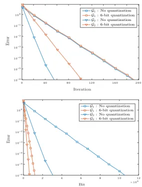
Figure 2.Comparison of the proposed algorithm for the gossip problem and the push-sum protocol using exact-communication based on iteration (Top) and total number of bits communicated between two neighbor nodes (Bottom) over the graphsG1andG2.
formly distributed random variables. Moreover we initialize the auxiliary parametersxbi =0andyi = 1for alli∈[n]. In Figure2(Top) we compare the performance of Algorithm
1with the push-sum protocol with exact-communication for both networksG1andG2. While Algorithm1has almost the same performance as push-sum overG1, it is outperformed by push-sum overG2.
However the superiority of exact-communication methods compared in each iteration could be predicted. In order to compare the two methods based on time spent to reach a specific level of error, we compare their performances based on the number of bits that each worker communicates. In Figure2(Bottom) the number of bits required to reach a certain error performance is illustrated for both methods. For the graphs G1 andG2 we observe up to 10x and 6x reduction in the total number of bits, respectively.
Decentralized optimization experiments.Next, we study the performance of Algorithm2for decentralized stochastic optimization using convex and non-convex objective func-tions. First, we consider the objective
f(x) = 1 2nm n X i=1 m X j=1 x−ζji 2 ,
where we setm=n= 10andd= 256. Thus each node i has access to its local data-set{ζi
1, ζ2i,· · ·, ζ10i } and is using one sample at random in each iteration to obtain the
0 20 40 60 80 100 10-2 10-1 100 101 0 1 2 3 4 5 6 7 8 9 10 105 10-1 100 101
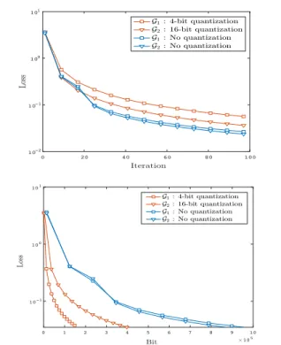
Figure 3.Comparison of the proposed method and exact-communication push-sum method using least-square as objective, based on the iteration number (Top) and total number of communi-cated bits over the graphsG1andG2.
stochastic gradient of its own local function. Here we use the data-set generated according to
ζjii.i.d.∼ ζ?+N(0,I256), for alli, j,
whereζ?is a fixed vector initialized asUniform[0,100]256. The step sizeαfor each setting, is fine-tuned up to iter-ation 50 among 20values in the interval [0.01,3]. The Loss at iterationTis presented by1dkez1(T)−ζoptk, where
e
z1(T) := T1 P T
t=1ez1(t)is the time-average of the model
of worker1andζoptis the optimal solution.
The results of this experiment are in Figure3(Top) which illustrates the convergence of Algorithm 2based on the number of iterations for different levels of quantization and over the two graphsG1andG2. The non-quantized method outperforms the quantized methods based on iteration. This is due to the quantization noise injected in the flow of in-formation over the graph which depends on the number of bits each node uses for encoding and the structure of graph. However this error asymptotically vanishes resulting in small overall quantization noise. This implies that with less quantization noise (i.e., using more bits to encode) the loss decay based on iteration number gets smaller. However as we observe in Figure3(Bottom), more quantization lev-els will result in larger number of bits required to achieve a certain level of loss. Consequently, the push-sum protocol
0 40 80 120 160 200 1 2 3 3.5 0 1 2 3 4 5 6 107 1.5 2 2.5 3 3.5
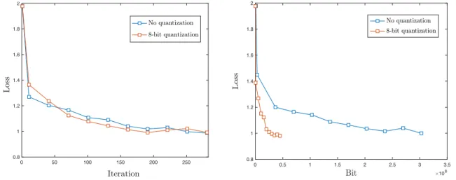
Figure 4.Comparison of the proposed method and exact-communication push-sum method in training a neural network with MNIST data-set, based on the iteration number (Top) and total number of communicated bits (Bottom).
with exact communication for optimization over directed graphs is not communication-efficient as we demonstrated that using smaller number of bits with Algorithm2results in5x reduction in transmitted bits.
As we showed in Theorem5.3in Section5, our proposed method guarantees convergence to a stationary point for non-convex and smooth objective functions. In order to illustrate this, we train a neural-network with10hidden units with sigmoid activation function to classify the MNIST data-set into10 classes. We use the graphG1 with10 nodes where each node has access to1000samples of data-set and uses a randomly selected mini-batch of size 10 for computing the local stochastic gradient descent. For each setting, the step-sizeαis fine-tuned up to iteration200and over15values in the interval[0.1, 3]. Figure4illustrates the results for training loss of two aforementioned methods based on number of iteration (Top) and total number of bits communicated between two neighbor nodes (Bottom). We note the close gap in each iteration between the loss decay of our proposed method with8bits quantization, and the push-sum with exact communication. However since our method uses significantly less bits in each iteration, it reaches the same training loss in fewer iterations. In particular Figure4
(Bottom) demonstrates5x reduction in total number of bits communicated using our proposed method.
7. Conclusion and Future Work
In this paper, we proposed a scheme for communication-efficient decentralized learning over directed graphs. We showed that our method converges at the same convergence rate as non-quantized methods for both gossip and decentral-ized optimization problems. As we demonstrated in Section
6, the proposed approach results in significant improve-ments in communication-time of the push-sum protocol. An interesting future direction is extending these results to algo-rithms that achieve linear convergence for strongly-convex problems (e.g., (Xi & Khan,2017)). Another direction is extending our results to asynchronous decentralized opti-mization over directed graphs.
Acknowledgements
This work was supported by National Science Foundation (NSF) under grant CCF-1909320 and UC Office of President under Grant LFR-18-548175.
References
Alistarh, D., Grubic, D., Li, J., Tomioka, R., and Vojnovic, M. Qsgd: Communication-efficient sgd via gradient quan-tization and encoding. InAdvances in Neural Information
Processing Systems, pp. 1709–1720, 2017.
Assran, M. and Rabbat, M. Asynchronous gradient-push.
IEEE Transactions on Automatic Control, 2020.
Assran, M., Loizou, N., Ballas, N., and Rabbat, M. Stochas-tic gradient push for distributed deep learning. arXiv
preprint arXiv:1811.10792, 2018.
Bernstein, J., Wang, Y.-X., Azizzadenesheli, K., and Anand-kumar, A. signsgd: Compressed optimisation for non-convex problems. arXiv preprint arXiv:1802.04434, 2018.
Blondel, V. D., Hendrickx, J. M., Olshevsky, A., and Tsit-siklis, J. N. Convergence in multiagent coordination, consensus, and flocking. InProceedings of the 44th IEEE
Conference on Decision and Control, pp. 2996–3000.
IEEE, 2005.
Doan, T. T., Maguluri, S. T., and Romberg, J. Accel-erating the convergence rates of distributed subgradi-ent methods with adaptive quantization. arXiv preprint
arXiv:1810.13245, 2018.
Jadbabaie, A., Lin, J., and Morse, A. S. Coordination of groups of mobile autonomous agents using nearest neigh-bor rules. IEEE Transactions on automatic control, 48 (6):988–1001, 2003.
Karimireddy, S. P., Rebjock, Q., Stich, S. U., and Jaggi, M. Error feedback fixes signsgd and other gradient compres-sion schemes.arXiv preprint arXiv:1901.09847, 2019. Kempe, D., Dobra, A., and Gehrke, J. Gossip-based
com-putation of aggregate information. In44th Annual IEEE Symposium on Foundations of Computer Science, 2003.
Proceedings., pp. 482–491. IEEE, 2003.
Koloskova, A., Stich, S. U., and Jaggi, M. De-centralized stochastic optimization and gossip algo-rithms with compressed communication.arXiv preprint
arXiv:1902.00340, 2019.
Lian, X., Zhang, C., Zhang, H., Hsieh, C.-J., Zhang, W., and Liu, J. Can decentralized algorithms outperform central-ized algorithms? a case study for decentralcentral-ized parallel stochastic gradient descent. InAdvances in Neural
Infor-mation Processing Systems, pp. 5330–5340, 2017.
Nedi´c, A. and Olshevsky, A. Distributed optimization over time-varying directed graphs. IEEE Transactions on
Au-tomatic Control, 60(3):601–615, 2014.
Nedic, A. and Ozdaglar, A. Distributed subgradient meth-ods for multi-agent optimization. IEEE Transactions on
Automatic Control, 54(1):48–61, 2009.
Nedic, A., Olshevsky, A., Ozdaglar, A., and Tsitsiklis, J. N. On distributed averaging algorithms and quantization ef-fects. IEEE Transactions on automatic control, 54(11): 2506–2517, 2009.
Nedic, A., Olshevsky, A., and Shi, W. Achieving geomet-ric convergence for distributed optimization over time-varying graphs. SIAM Journal on Optimization, 27(4): 2597–2633, 2017.
Pu, S., Shi, W., Xu, J., and Nedic, A. Push-pull gradient methods for distributed optimization in networks. IEEE
Transactions on Automatic Control, 2020.
Reisizadeh, A., Taheri, H., Mokhtari, A., Hassani, H., and Pedarsani, R. Robust and communication-efficient col-laborative learning. InAdvances in Neural Information
Processing Systems, pp. 8386–8397, 2019.
Saber, R. O. and Murray, R. M. Consensus protocols for networks of dynamic agents. 2003.
Shi, W., Ling, Q., Wu, G., and Yin, W. Extra: An exact first-order algorithm for decentralized consensus optimization.
SIAM Journal on Optimization, 25(2):944–966, 2015.
Stich, S. U. Local sgd converges fast and communicates little. arXiv preprint arXiv:1805.09767, 2018.
Tsianos, K. I., Lawlor, S., and Rabbat, M. G. Push-sum distributed dual averaging for convex optimization. In
2012 ieee 51st ieee conference on decision and control
(cdc), pp. 5453–5458. IEEE, 2012.
Wang, J., Tantia, V., Ballas, N., and Rabbat, M. Slowmo: Improving communication-efficient distributed sgd with slow momentum. arXiv preprint arXiv:1910.00643, 2019.
Xi, C. and Khan, U. A. On the linear convergence of dis-tributed optimization over directed graphs.arXiv preprint
arXiv:1510.02149, 2015.
Xi, C. and Khan, U. A. Dextra: A fast algorithm for op-timization over directed graphs. IEEE Transactions on
Automatic Control, 62(10):4980–4993, 2017.
Xi, C., Wu, Q., and Khan, U. A. On the distributed opti-mization over directed networks.Neurocomputing, 267: 508–515, 2017.
Xi, C., Mai, V. S., Xin, R., Abed, E. H., and Khan, U. A. Linear convergence in optimization over directed graphs with row-stochastic matrices.IEEE Transactions on
Au-tomatic Control, 63(10):3558–3565, 2018.
Xiao, L. and Boyd, S. Fast linear iterations for distributed averaging.Systems & Control Letters, 53(1):65–78, 2004. Xin, R. and Khan, U. A. A linear algorithm for optimization
over directed graphs with geometric convergence. IEEE
Control Systems Letters, 2(3):315–320, 2018.
Yuan, K., Ling, Q., and Yin, W. On the convergence of decentralized gradient descent. SIAM Journal on
Opti-mization, 26(3):1835–1854, 2016.
Zeng, J. and Yin, W. Extrapush for convex smooth decentral-ized optimization over directed networks. arXiv preprint
Appendix
In this section, we first provide further numerical experiments as well as presenting the hyper-parameters of all methods used in the experiments. We then continue with presenting proofs of the Theorems5.1-5.3.
7.1. Neural Network Training on CIFAR-10 dataset
We train a neural network of 20 hidden-units with sigmoid activation functions for binary classification of the CIFAR-10 dataset. We use the topology ofG1as in Figure1with the corresponding weight matrix constructed according to Example1. The value of step sizeαis fine-tuned among 15 values ofαuniformly selected in[0.1,3]and up to iteration 300 for both algorithms. 0 50 100 150 200 250 0.8 1 1.2 1.4 1.6 1.8 2 0 0.5 1 1.5 2 2.5 3 3.5 108 0.8 1 1.2 1.4 1.6 1.8 2
Figure 5.Comparison of the proposed method and exact-communication push-sum method in training a neural network with CIFAR-10 data-set, based on the iteration number (Left) and total number of bits communicated between two neighbor nodes (Right).
Figure5illustrates the performance of the proposed algorithm based on iteration number (Left) and number of bits commu-nicated between two neighbor nodes (Right), and compares the vanilla push-sum method and the proposed communication-efficient method with 8 bits for quantization. We use SGD with mini-batch size of 100 samples for each node in both methods. We highlight the close similarity in training loss of the two methods for a fixed number of iteration. More importantly the proposed method uses remarkably smaller number of bits implying faster communication while reaching the same level of training loss.
7.2. Details of the Numerical Experiments
The step-sizes of the algorithms used in Section6are fine tuned over the interval[0.01,3], so that the best error achieved by each method is compared. In Table1we present the fine-tuned step sizes as well as model size (i.e. dimension of parameteres) and the mini-batch size of the algorithms that are used throughout the numerical experiments.
Table 1.Details on the hyper-parameters of the vanilla push-sum algorithm with no quantization and the proposed quantized push-sum algorithm.
OBJECTIVE ITERATION MODEL SIZE MINI-BATCH SIZE GRAPH STEP SIZE
SQUARE LOSS 50 256 1 G1 1.7
SQUARE LOSS 50 256 1 G2 1.1
NN, MNIST 200 7960 10 G1 2.2
NN, CIFAR-10 300 20542 100 G1 1.1
SQUARE LOSS(4-BITS) 50 256 1 G1 1.1
SQUARE LOSS(16-BITS) 50 256 1 G2 1.1
NN, MNIST (8-BITS) 200 7960 10 G1 1.9
Proofs
NotationThroughout this section we set the following notation. For variables, stochastic gradients and gradients, we concatenate the row vectors corresponding to each node to form the following matrices:
Z(t) := [z1(t) ; z2(t) · · · zn(t)]∈Rn×d,
∂F(Z(t), ζt) := [∇F1(z1(t), ζ1,t) ; ∇F2(z2(t), ζ2,t) · · · ∇Fn(zn(t), ζn,t)]∈Rn×d, ∂f(Z(t)) := [∇f1(z1(t)) ; ∇f2(z2(t)) · · · ∇fn(zn(t))]∈Rn×d.
8. Proof of Theorem
5.1
: Quantized Gossip over Directed Graphs
First we write the iterations of Algorithm1in matrix notation to derive the following: Q(t) =QX(t)−Xb(t) b X(t+ 1) =Xb(t) +Q(t) X(t+ 1) =X(t) + (A−I)Xb(t+ 1) y(t+ 1) =Ay(t) zi(t+ 1) = xi(t+1) yi(t+1) (11)
Based on this, we can rewrite the update rule forX(t+ 1)as follows:
X(t+ 1) =AX(t) + (A−I)(Xb(t+ 1)−X(t)).
By repeating this forX(t), ..., X(1), the update rule forX(t+ 1)takes the following shape:
X(t+ 1) =AtX(1) +
t−1
X
s=0
A(A−I)(X(t−s+ 1)−X(t−s)). (12) Multiplying both sides by1T and recalling that1TA=1T, yields that
1TX(t+ 1) =1TX(1). (13)
With this and (12) we have for allt≥1:
X(t+ 1)−φ1TX(1) = AtX(1) + t−1 X s=0 As(A−I)(Xb(t−s+ 1)−X(t−s))−φ1TX(1) 6Cλt X(1) + 2C t−1 X s=0 λs b X(t−s+ 1)−X(t−s) . (14)
Furthermore by the iterations of Algorithm11as well as the assumption on quantization noise in Assumption3we find that E X(t+ 1)−Xb(t+ 2) =E X(t+ 1)−Xb(t+ 1)−Q(t+ 1) ≤ω X(t+ 1)−Xb(t+ 1) =ω X(t) + (A−I)Xb(t+ 1)−Xb(t+ 1) ≤ω X(t)−Xb(t+ 1) +ω (A−I)Xb(t+ 1) .
Next, we add and subtract(A−I)X(t)to the RHS and also use the fact thatAφ=φ( (Zeng & Yin,2015)) to conclude that E X(t+ 1)−Xb(t+ 2) ≤ω X(t)−Xb(t+ 1) +ω (A−I)(Xb(t+ 1)−X(t)) +ω (A−I)X(t)−φ1TX(1) . (15)
Letγ:=kA−Ik, λ1:=ω(1 +γ)andλ01:=ωγ, then we conclude that
E X(t+ 1)−Xb(t+ 2) =λ1 b X(t+ 1)−X(t) +λ01 X(t)−φ1TX(1) . Denoting byR(t) :=E X(t)−φ1TX(1) andU(t) =E b X(t+ 1)−X(t)
, we derive the next two inequalities based on (14) and (15):
(
ER(t+ 1)≤C·λtkX(1)k+2CPt−s=01λsU(t−s) EU(t+ 1)≤λ1U(t) +λ01R(t)
(16)
Lemma 8.1. The iterates ofU(t)satisfy for all iterationst≥1
U(t)≤ξ1λt/2,
whereξ1= max{4λCλ1kX(1)k, λ1kXλ1/(1)2 k}and for the values ofλ1chosen such thatλ1≤
1 2( 1 λ1/2 + 2C λ−λ3/2) −1.
Proof. Noting thatλ01≤λ1, we have by (16) for allt≥1:
U(t+ 1)≤λ1U(t) + 2C·λ1 λt−1kX(1)k+ t−2 X s=0 λsU(t−s−1) ! . (17)
The proof is based on induction on the inequality in (17). LetU(t)≤ξ1·λt/2, then by (17)
U(t+ 1)≤λ1·ξ1·λt/2+ 2Cλ1 λt−1kX(1)k + 2Cλ1·ξ1· λt−21 1−λ1/2 = λ1·ξ1 λ1/2 λ t+1 2 + 2Cλ1 kX(1)k·λt−23 λt+12 +2C·λ1·ξ1 λ−λ3/2 λ t+1 2 ≤λ1ξ1 1 λ1/2 + 2C λ−λ3/2 λt+12 +2C·λ1kX(1)k λ ·λ t+1 2 ≤ 1 2ξ1+ 2C·λ1kX(1)k λ ·λt+12 ≤ξ1λ t+1 2 ,
where the last two steps follow by the assumptions of the lemma onξ1andλ1. Moreover forU(1)we follow the inequalities similar to (15) to find that
U(1)≤ωkX(1)k≤ξ1λ1/2,
where we usedω≤λ1in the last inequality. This completes the proof of the lemma.
Lemma8.1implies that the quantization errorU(t)is decaying with the rateλt/2. As we will see shortly, this results in total error, decaying with the same rate. From the update rule in Algorithm11, we obtain the following for allt≥0:
Since by assumptiony(1) =1it yields that
y(t+ 1) =At1=At−φ1T1+φ1T1
=At−φ1T1+φn. Therefore for alli∈[n]
yi(t+ 1) =
h
At−φ1Ti i
+φin. Furthermore, based on Algorithm11the parameterzi(t+ 1)satisfies:
zi(t+ 1) = xi(t+ 1) yi(t+ 1) = h AtX(1) +Pt−1 s=0A s(A−I) b X(t−s+ 1)−X(t−s)i i h At−φ1T1i i +φin . (18)
Using this, we find the following expression for the vector representing error of nodei:
zi(t+ 1)− 1TX(1) n = h AtX(1) +Pt−1 s=0A s(A−I)( b X(t−s+ 1)−X(t−s))i i nh(At−φ1T)1i i +φin − 1TX(1)hAt−φ1T1i i +φin nh(At−φ1T)1i i +φin = nhAt−φ1Ti i X(1) +nPt−1 s=0[A s(A−I)] i(Xb(t−s+ 1)−X(t−s))−1TX(1) h (At−φ1T)i i 1 nhAt−φ1Ti i 1+φin .
By Proposition2.1it holds thatAt1≥δand
[A t−φ1T ]i ≤Cλ
tfor allt≥1; thus, we derive the following for the error of parameter of nodei:
E zi(t+ 1)− 1TX(1) n ≤ C δ ·λ t X(1) + C δ t−1 X s=0 λs·ξ1·λ t−s 2 + C nδλ t 1 T X(1) ≤ C δ ·λ t X(1) + C nδλ t 1 TX(1) · √ n+C δξ1· λt/2 1−λ1/2. Note thatk1TX(1)k≤ kX(1)k·√n. Thus,
E zi(t+ 1)−1 T X(1) n ≤2C δ λ t X(1) + C δ · ξ1 1−λ1/2λ t/2.
Rewriting the condition onλ1in Lemma8.1based onω, we derive the inequality in the statement of Theorem5.1.
9. Proof of Theorem
5.2
: Quantized Push-sum with Convex Objectives
First we write the iterations of Algorithm2in matrix notation to derive the following:
Q(t) =QX(t)−Xb(t) b X(t+ 1) =Xb(t) +Q(t) W(t+ 1) =X(t) + (A−I)Xb(t+ 1) y(t+ 1) =Ay(t) zi(t+ 1) = wi(t+1) yi(t+1) X(t+ 1) =W(t+ 1)−α ∂F(Z(t+ 1), ζt+1) (19)
Similar to (14), we can rewrite the iterations ofX(t)to obtain the following expression: (20) X(t+ 1)−φ1 T X(t) 2 ≤3C2λ2t X(1) 2 + 3C2α2 t X s=0 λs ∂F(Z(t−s+ 1), ζt−s+1) 2 + 3C2 t−1 X s=0 λs Xb(t−s+ 1)−X(t−s) 2
For the last term, we expand the summation as well as simplifying the resulting expressions to obtain:
t−1 X s=0 λs Xb(t−s+ 1)−X(t−s) 2 = t−1 X s=0 λ2s Xb(t−s+ 1)−X(t−s) 2 +X s6=s0 λs·λs0 Xb(t−s+ 1)−X(t−s) Xb(t−s 0+ 1)−X(t−s0)
Using the relationx·y≤x2/2 +y2/2for allx, y∈
R, as well as the inequalityλ2s≤ λ
s
1−λ, from the equation above the following yields: t−1 X s=0 λs Xb(t−s+ 1)−X(t−s) 2 ≤ t−1 X s=0 λ2s Xb(t−s+ 1)−X(t−s) 2 + 1/2X s6=s0 λs+s0 Xb(t−s+ 1)−X(t−s) 2 + 1/2X s6=s0 λs·λs0 Xb(t−s 0+ 1)−X(t−s0) 2 ≤ t−1 X s=0 λ2s+ λ s 1−λ Xb(t−s+ 1)−X(t−s) 2 ≤ t−1 X s=0 2λs 1−λ Xb(t−s+ 1)−X(t−s) 2 .
Using a similar approach as above, we can bound the second term in the RHS of (20) as follows:
t X s=0 λs ∂F(Z(t−s+ 1), ζt−s+1) 2 ≤ t X s=0 2λs 1−λ ∂F(Z(t−s+ 1), ζt−s+1) 2 .
Thus from (20) with the assumption thatX(1) = 0(as in Assumption4) we find that
E X(t+ 1)−φ1 T X(t) 2 ≤6C2E t−1 X s=0 λs 1−λ Xb(t−s+ 1)−X(t−s) 2 + 6C2α2 t−1 X s=0 λs 1−λE ∂F(Z(t−s+ 1), ζt−s+1) 2 ≤6C2 t−1 X s=0 λs 1−λE Xb(t−s+ 1)−X(t−s) 2 +6C 2α2nD2 (1−λ)2 , (21)
(15) derived for Algorithm11, we derive the following inequality here in the presence of stochastic gradients: E X(t+ 1)−Xb(t+ 2) 2 ≤3ω2 1 +γ2E X(t)−Xb(t+ 1) 2 + 3ω2γ2E X(t)−φ1 T X(t−1) 2 + 3ω2α2E ∂F(Z(t+ 1), ζt+1) 2 . (22) Letλ2 :=ω2(1 +γ2). Then, from (22) as well as bounding stochastic gradients according to Assumption6, it directly follows that E X(t+ 1)−Xb(t+ 2) 2 ≤3λ2 E X(t)−Xb(t+ 1) 2 +E X(t)−φ1 T X(t−1) 2 +nα2D2 . (23) LetR(t+ 1) :=E X(t+ 1)−φ1 T X(t) 2 andU(t+ 1) :=E X(t+ 1)−Xb(t+ 2) 2
. Then noting (21) and (23), we can rewrite the corresponding errors as follows:
( ER(t+ 1)≤ 6C 2nα2D2 (1−λ)2 + 6C2 1−λ Pt−1 s=0λ sU(t−s), EU(t+ 1)≤3λ2 U(t) +R(t) +nα2D2 . (24) Next, we state the following lemma which shows that the error of quantization i.e.U(t)decays proportionately withα2. Lemma 9.1. Under Assumption4, the inequalities in(24)satisfy the following for allλ2 ≤ (16 + C
2 (1−λ)2)−1and all iterationst≥1 U(t)≤ξ2α2, (25) whereξ2= 6λ2 nD2+6(1nC−λ2D)22 .
Proof. First we write the inequalities in (24) based onU(·)to obtain:
U(t+ 1)≤3λ2 U(t) +nα2D2+6nC 2α2D2 (1−λ)2 + 6C2 1−λ t−2 X s=0 λsU(t−s−1).
Thus, by the assumption of induction we obtain the following forU(t+ 1):
U(t+ 1)≤3λ2 ξ2α2+nα2D2+ 6C2α2nD2 (1−λ)2 + 6C2ξ 2α2 (1−λ) t−2 X s=0 λs ! ≤3λ2α2ξ2 1 + 6C 2 (1−λ)2 + 3λ2α2 nD2+6nC 2D2 (1−λ)2 ≤ξ2α 2 2 + 3λ2α 2 nD2+6nC 2D2 (1−λ)2 =ξ2α2, (26)
where the last two steps follow from the assumptions forλ2andξ2, respectively. Note that based on iterations of the algorithm and Assumption4we conclude thatkU(1)k= 0. This completes the proof of the lemma.
Lemma 9.2. Under Assumptions1-7, ifλ2 ≤(16 + C
2
(1−λ)2)−
1, the following relation holds for the consensus error of
Algorithm2for allt≥1:
E zi(t+ 1)− 1TX(t) n 2 ≤ 6C 2α2 δ2(1−λ)2(2nD 2+ξ 2), whereξ2= 6λ2 nD2+6nC2D2 (1−λ)2 .
Proof. Using the update rule in Algorithm19and similar to (18) we derive the following for the vector corresponding to consensus error of nodei:
zi(t+ 1)− 1TX(t) n = h Pt−1 s=0A s(A−I)( b X(t−s+ 1)−X(t−s))−αPt s=0A s∂FZ(t−s+ 1), ζt−s +1 i i h (At−φ1T) 1i i +φin + α1TPt−1 s=0∂F Z(t−s+ 1), ζt−s+1 h At−φ1T1i i +φin nh(At−φ1T)1i i+φin .
Note that by Proposition2.1for allt≥1we have[(At−φ1T)1]
i+φin= [At1]i ≥δ, which yields the following for squared norm of consensus error:
E zi(t+ 1)− 1TX(t) n 2 ≤ 3 δ2E t X s=0 h As(A−I)i i b X(t−s+ 1)−X(t−s) 2 +3α 2 δ2 E t X s=0 h As−φ1Ti i ∂FZ(t−s+ 1), ζt−s+1 2 +3α 2 n2δ2E 1T t−1 X s=0 h At−φ1Ti i ∂FZ(t−s+ 1), ζt−s+1 ! 2 . (27)
By expanding the first term in the RHS of (27) we derive
t X s=0 h As(A−I)i i b X(t−s+ 1)−X(t−s) 2 = t X s=0 h As(A−I)i i b X(t−s+ 1)−X(t−s) 2 + t X s6=s0 h As(A−I)i i b X(t−s+ 1)−X(t−s),hAs(A−I)i i b X(t−s0+ 1)−X(t−s0) ≤ t X s=0 h As(A−I)i i 2 b X(t−s+ 1)−X(t−s) 2 + t X s6=s0 h As(A−I)i i b X(t−s+ 1)−X(t−s) h As(A−I)i i b X(t−s0+ 1)−X(t−s0) .
Using the relationx·y≤x2/2 +y2/2for allx, y∈
R, this inequality reduces to the following:
t X s=0 h As(A−I)i i b X(t−s+ 1)−X(t−s) 2 ≤ t X s=0 h As(A−I)i i 2 b X(t−s+ 1)−X(t−s) 2 +1 2 t X s6=s0 h As(A−I)i i h As0(A−I)i i b X(t−s+ 1)−X(t−s) 2 + b X(t−s0+ 1)−X(t−s0) 2! .
Next we use Proposition2.1to yield that t X s=0 h As(A−I)i i b X(t−s+ 1)−X(t−s) 2 ≤ C2 t X s=0 λ2s b X(t−s+ 1)−X(t−s) 2 +C2 t X s6=s0 λs+s0 b X(t−s+ 1)−X(t−s) 2 ≤C2 t X s=0 λ2s+ λ s 1−λ b X(t−s+ 1)−X(t−s) 2 ≤ 2C 2 1−λ t X s=0 λs b X(t−s+ 1)−X(t−s) 2 , where we usedλ2s≤ λs
1−λ to derive the last inequality. Using the same approach for the second term in the RHS of (27), we derive the following upper bound:
E t X s=0 h As−φ1Ti i∂F Z(t−s+ 1), ζt−s+1 2 ≤ 2C 2 1−λ t X s=0 λsE ∂F(Z(t−s+ 1), ζt−s+1) 2 .
To bound the third term in the RHS of (27), we use the same method,as well as the fact thatkAt−φ1Tk≤λt≤λsfor all s≤tto deduce that E 1T t−1 X s=0 h At−φ1Ti i ∂FZ(t−s+ 1), ζt−s+1 ! 2 ≤ 2nC 2 1−λ t X s=0 λsE ∂F(Z(t−s+ 1), ζt−s+1) 2 .
Replacing these back in (27) gives
E zi(t+ 1)− 1TX(t) n 2 ≤ 6C 2 δ2(1−λ) t X s=0 λsE b X(t−s+ 1)−X(t−s) 2 + 6α2C2 δ2(1−λ)+ 6α2C2 nδ2(1−λ) t X s=0 λsE ∂F(Z(t−s+ 1), ζt−s+1) 2 . (28) Note thatU(t−s) :=E b X(t−s+ 1)−X(t−s) 2
≤ξ2α2by Lemma9.1. Also by bounded stochastic gradient property in Assumption6, we haveE ∂F(Z(t−s+ 1), ζt−s+1) 2
≤nD2.Therefore we conclude the following from (28):
E zi(t+ 1)− 1TX(t) n 2 ≤ 6ξ2C 2α2 δ2(1−λ)2 + 6α2C2 δ2(1−λ)2 + 6α2C2 nδ2(1−λ)2 nD2. (29) Simplifying relations with1 + 1/n≤2, yields the desired inequality in the statement of the lemma.
We continue with proving the next lemma which relates the consensus error as stated in Lemma9.2to the error of global objective functionfevaluated at the average of parametersxi(t)of all nodes.
Lemma 9.3. For allt≥1, iterations of Algorithm19satisfy:
E ¯ X(t+ 1)−z? 2 ≤E ¯ X(t)−z? 2 − 2α−8α 2L n E(f X¯(t))−f(z?) +2αL+ 4L 2α2 n n X i=1 E zi(t+ 1)− ¯ X(t) + 2σ2α2 n .
Proof. First we recall thatAis column stochastic; thus, it yields that1T(A−I) = 0. Therefore, iterations of Algorithm19 yield that ¯ X(t+ 1) = ¯X(t)−α n n X i=1 ∇Fi(zi(t+ 1), ζi,t+1). Thus, EX¯(t+ 1)−z ? 2 =E X¯(t)−z ? 2 −2α n n X i=1 E D ∇fi(zi(t+ 1)),X¯(t)−z? E +α2E 1 n n X i=1 ∇Fi(zi(t+ 1), ζi,t+1) 2 . (30)
We derive an upper bound for the third term by adding and subtracting 1nPn
i=1∇fi(zi(t+ 1)): E 1 n n X i=1 ∇Fi(zi(t+ 1), ζi,t+1) 2 ≤2E 1 n n X i=1 (∇Fi(zi(t+ 1), ζi,t+1)− ∇fi(zi(t+ 1))) 2 + 2E 1 n n X i=1 ∇fi(zi(t+ 1)) 2 ≤ 2 n2 n X i=1 E ∇Fi(zi(t+ 1), ζi,t+1)− ∇fi(zi(t+ 1)) 2 + 2E 1 n n X i=1 ∇fi(zi(t+ 1)) 2 ≤ 2σ 2 n + 2E 1 n n X i=1 ∇fi(zi(t+ 1)) 2 . (31)
For the last term in (31) we have
E 1 n n X i=1 ∇fi(zi(t+ 1)) 2 ≤2E 1 n n X i=1 (∇fi(zi(t+ 1))− ∇fi( ¯X(t))) 2 + 2E 1 n n X i=1 (∇fi( ¯X(t))− ∇fi(z?)) 2 ≤ 2 n n X i=1 E ∇fi(zi(t+ 1))− ∇fi( ¯X(t)) 2 + 2E ∇f( ¯X(t))− ∇f(z?) 2 ≤2L 2 n n X i=1 E zi(t+ 1)− ¯ X(t) 2 +4L n (Ef( ¯X(t))−f(z ?)).
Replacing this back in (31) we have
E 1 n n X i=1 ∇Fi(zi(t+ 1), ζi,t+1) 2 ≤ 2σ 2 n + 4L2 n n X i=1 E zi(t+ 1)− ¯ X(t) 2 +8L n (Ef( ¯X(t))−f(z ?)). (32)
Next, we will achieve a bound for the second term in the RHS of (30). By adding and subtractingzi(t+ 1)we have E D ∇fi(zi(t+ 1)),X¯(t)−z? E =E D ∇fi(zi(t+ 1)),X¯(t)−zi(t+ 1) E +E D ∇fi(zi(t+ 1)),zi(t+ 1)−z? E , (33) where after usingL-smoothness of the functionfifor the first term and convexity of the functionfifor the second term of (33) we deduce that E D ∇fi(zi(t+ 1)),X¯(t)−z? E ≥Efi( ¯X(t))−Efi(zi(t+ 1))− L 2E ¯ X(t)−zi(t+ 1) 2 +Efi(zi(t+ 1))−fi(z?) =Efi( ¯X(t))−fi(z?)−L 2E ¯ X(t)−zi(t+ 1) 2 .
Using this and recalling thatf(·) = n1Pn
i=1fi(·), we derive the following:
−2α n n X i=1 E D ∇fi(zi(t+ 1)),X¯(t)−z? E ≤ −2α(Ef( ¯X(t))−f(z?)) + 2αL n n X i=1 E ¯ X(t)−zi(t+ 1) 2 .
By replacing this result and (32) in (30) we derive the desired inequality in the statement of the lemma. We continue with rearranging and summing both sides of Lemma9.3fort= 1,· · ·, T to find the following:
2α−8α 2L n T X t=1 (Ef( ¯X(t))−f(z?)) ≤ ¯ X(1)−z? 2 +2αL+ 4α 2L2 n T X t=1 n X i=1 E zi(t+ 1)− ¯ X(t) 2 + T X t=1 2σ2α2 n . Scaling both sides, as well as noting the Assumption4i.e.X(1) = 0, we find that
1 T T X t=1 (Ef( ¯X(t))−f(z?)) ≤ 1 2T α(1−4αL n ) kz?k2+ 2αL 2+L nT(1−4αL n ) T X t=1 n X i=1 E zi(t+ 1)− ¯ X(t) 2 + ασ 2 n(1−4αL n ) .
Using convexity off(·), the above inequality simplifies to the following:
Ef 1 T T X t=1 ¯ X(t) ! −f(z?) ≤ 1 2T α(1−4αL n ) kz?k2+ 2αL 2+L nT(1−4αL n ) T X t=1 n X i=1 E zi(t+ 1)− ¯ X(t) 2 + ασ 2 n(1−4αL n ) ,
which after replacing the consensus error from Lemma9.2, further simplifies into
Ef 1 T T X t=1 ¯ X(t) ! −f(z?) ≤ 1 2T α(1−4αL n ) kz?k2+6α 2C2(2nD+ξ 2) δ2(1−λ)2 · 2αL2+L 1−4αL n + ασ 2 n(1−4αL n ) . (34)
The inequality in (34) guarantees the convergence of time average of X¯(t) = 1 n
Pn
i=1xi(t)to the optimal pointz?. However computing the average ofxi(t)between workers in every iteration is time consuming since it can not be done in the decentralized setting. Next we show that the time average of the local variables,zi(t)converges to an optimalz?, for every nodei. First, ByL-smoothness of the functionf(·)as well as the inequalityhx,yi ≤1
2kxk 2+1
2kyk
2, we derive for alli∈[n]it holds that
f 1 T T X t=1 zi(t+ 1) ! −f 1 T T X t=1 ¯ X(t) ! ≤ * 1 T T X t=1 zi(t+ 1)−X¯(t),∇f 1 T T X t=1 ¯ X(t) !+ + L 2T2 T X t=1 zi(t+ 1)−X¯(t) 2 ≤ 1 2T2 T X t=1 zi(t+ 1)−X¯(t) 2 +1 2 ∇f 1 T T X t=1 ¯ X(t) ! 2 + L 2T2 T X t=1 zi(t+ 1)−X¯(t) 2 . (35)
Note that for the optimal solutionz? it holds thatk∇f(x)k2= k∇f(x)− ∇f(z?)k2≤2L(f(x)−f(z?)). Using this inequality for the second term in (35) we conclude that
Ef 1 T T X t=1 zi(t+ 1) ! −Ef 1 T T X t=1 ¯ X(t) ! ≤ 1 2T + L 2T T X t=1 E zi(t+ 1)− ¯ X(t) 2 +L Ef 1 T T X t=1 ¯ X(t) ! −f(z?) ! . (36)
By replacing the consensus error as derived in (29) and combining the inequalities (34) and (36), we get the convergence error of the time average of local variableszi:
Ef 1 T T X t=1 zi(t+ 1) ! −f(z?) ≤ L+ 1 2T α(1−4αL n ) kz?k2+ (2αL 2+L)(L+ 1) 1−4αL n +1 +L 2 ! 6α2C2(2nD+ξ 2) δ2(1−λ)2 +ασ 2(L+ 1) n(1−4αL n ) . (37) We chooseα= √ n 8L√T in (37), which results in 1− 4αL n −1
≤2for allT ≥1andn≥1. Furthermore,
Ef 1 T T X t=1 zi(t+ 1) ! −f(z?) ≤ 8L√(L+ 1) nT kz ?k2 +σ 2(L+ 1) 4L√nT + C2n(L+ 1)L√n 2√T +L+ 1 ξ2+ 2nD2 10T δ2(1−λ)2L2 . (38) Replacingξ2and rewriting the condition onλ2withω(as required by Lemmas9.1and9.2) completes the proof.
10. Proof of Theorem
5.3
: Quantized Push-sum with Non-convex Objectives
Using theL-smoothness of the global objective function which is implied by Assumption5, we have for allt≥1:
Ef 1 TX(t+ 1) n ! =Ef 1 TX(t) n −α 1T∂F(Z(t+ 1, ζt+1)) n ! =Ef 1 TX(t) n ! −αE * ∇f 1 TX(t) n ! ,1 T∂f(Z(t+ 1)) n + +α 2L 2 E 1T∂F(Z(t+ 1, ζt+1)) n 2 . (39)
For the last term in the RHS of (39) we add and subtract 1nT∂f(Z(t+ 1))to yield
E 1T∂F(Z(t+ 1), ζt+1) n 2 =E 1T n ∂F(Z(t+ 1), ζt+1)−∂f(Z(t+ 1)) +1 T n ∂f(Z(t+ 1)) 2 =E 1T n ∂F(Z(t+ 1), ζt+1)−∂f(Z(t+ 1)) 2 +E 1T n ∂f(Z(t+ 1)) 2 + 2E * 1T n ∂F(Z(t+ 1), ζt+1)−∂f(Z(t+ 1)) ,1 T n∂f(Z(t+ 1)) + .
Since stochastic gradients of all nodes are unbiased estimators of the local gradients, the last term is zero in expectation. Thus, E 1T∂F(Z(t+ 1), ζt+1) n 2 ≤E 1T n ∂F(Z(t+ 1), ζt+1)−∂f(Z(t+ 1)) 2 +E 1T n∂f(Z(t+ 1)) 2 +2E * Eζt+1 1T n ∂F(Z(t+ 1), ζt+1)−∂f(Z(t+ 1)) ,1 T n ∂f(Z(t+ 1)) + =E 1T n ∂F(Z(t+ 1), ζt+1)−∂f(Z(t+ 1)) 2 +E 1T n ∂f(Z(t+ 1)) 2 . Next, by expanding and using the fact that stochastic gradients are computed independently among different nodes, we show that the first term in the equation above is bounded:
E 1T n ∂F(Z(t+ 1), ζt+1)−∂f(Z(t+ 1)) 2 = 1 n2E n X i=1 ∇Fi(zi(t+ 1), ζi,t+1)− ∇fi(zi(t+ 1)) 2 = 1 n2E n X i=1 ∇Fi(zi(t+ 1), ζi,t+1)− ∇fi(zi(t+ 1)) 2 + 1 n2E X i6=i0 ∇Fi(zi(t+ 1), ζi,t+1)− ∇fi(zi(t+ 1)),∇Fi0(zi0(t+ 1), ζi0,t+1)− ∇fi0(zi0(t+ 1)) = 1 n2E n X i=1 ∇Fi(zi(t+ 1), ζi,t+1)− ∇fi(zi(t+ 1)) 2 + 1 n2E X i6=i0
Eζi,t+1∇Fi(zi(t+ 1), ζi,t+1)− ∇fi(zi(t+ 1)),∇Fi0(zi0(t+ 1), ζi0,t+1)− ∇fi0(zi0(t+ 1))
= 1 n2E n X i=1 ∇Fi(zi(t+ 1), ζi,t+1)− ∇fi(zi(t+ 1)) 2 ≤ σ 2 n ,
where we recall Assumption7in the last inequality. Next, we rewrite (39) using the new terms as follows: Ef 1TX(t+ 1) n ! ≤Ef 1 TX(t) n ! −αE * ∇f 1 TX(t) n ! ,1 T∂f(Z(t+ 1)) n + +α 2L 2 σ2 n +E 1T n ∂f(Z(t+ 1)) 2 . (40)
Moreover, using the relationhx,yi=1 2kxk
2+1 2kyk
2−1
2kx−yk
2, we find the following for the second term in the RHS of (40): E * ∇f 1 TX(t) n ! ,1 T∂f(Z(t+ 1)) n + =1 2E ∇f 1 TX(t) n ! 2 +1 2E 1T∂f(Z(t+ 1)) n 2 −1 2E ∇f 1 TX(t) n ! −1 T∂f(Z(t+ 1)) n 2 . (41)
UsingL-lipschitz assumption of local gradients (Assumption5), the last term in (41) reduces to
E ∇f 1 T X(t) n ! −1 T ∂f(Z(t+ 1)) n 2 ≤1 n n X i=1 E ∇fi 1 T X(t) n ! − ∇fi(zi(t+ 1)) 2 ≤L 2 n n X i=1 E 1TX(t) n −zi(t+ 1) 2 ,
where we used∇f(x) = 1nPn
i=1∇fi(x)in the first step. Replacing this in (41) and finally substituting the resulting expression of (41) in (40) yields Ef 1 T X(t+ 1) n ! ≤Ef 1 T X(t) n ! +α 2σ2L 2n +α 2L−α 2 E 1T∂f(Z(t+ 1)) n 2 −α 2 E ∇f 1 T X(t) n ! 2 +αL 2 n n X i=1 E zi(t+ 1)− 1TX(t) n 2 . (42)
By replacing the value of consensus error from Lemma9.2in (42), we obtain the following:
Ef 1TX(t+ 1) n ! ≤Ef 1 TX(t) n ! +α 2σ2L 2n +α 2L−α 2 E 1T∂f(Z(t+ 1)) n 2 −α 2 E ∇f 1 T X(t) n ! 2 + 6α 3C2L2 δ2(1−λ)2 nD 2+D2+ξ 2. (43)
Thus by rearranging terms in (43) and averaging both sides fromt= 1tot=Twe conclude that
1−αL T T X t=1 E 1T∂f(Z(t+ 1)) n 2 + 1 T T X t=1 E ∇f 1 TX(t) n ! 2 ≤ 2 f 1T X(1) n −f? αT + ασ2L n + 12α2L2C2 δ2(1−λ)2 ξ2+nD 2+D2 . (44) By choosingα= √ n
L√T and noting thatX(1) = 0we derive the desired statement of the theorem. Note thatT ≥4nimplies that 1−αLT ≥ 1
2T guaranteeing that the first term in the LHS of (44) is positive. The consensus error in (10) is concluded from Lemma9.2with the given choice of step-size as in the statement of the theorem. This completes the proof of the theorem.