Automated Image Forgery Detection through
Classification of JPEG Ghosts
Fabian Zach, Christian Riess and Elli Angelopoulou
Pattern Recognition Lab University of Erlangen-Nuremberg
{riess,elli}@i5.cs.fau.de
Abstract. We present a method for automating the detection of the so-called JPEG ghosts. JPEG ghosts can be used for discriminating single-and double JPEG compression, which is a common cue for image manip-ulation detection. The JPEG ghost scheme is particularly well-suited for non-technical experts, but the manual search for such ghosts can be both tedious and error-prone. In this paper, we propose a method that au-tomatically and efficiently discriminates single- and double-compressed regions based on the JPEG ghost principle. Experiments show that the detection results are highly competitive with state-of-the-art methods, for both, aligned and shifted JPEG grids in double-JPEG compression.
1
Introduction
The goal of blind image forensics is to determine the authenticity of an im-age without using an embedded security scheme. With the broad availability of digital images and tools for image editing, it becomes increasingly important to detect malicious manipulations. Consequently, image forensics has recently gained considerable attention. Most existing methods fall into two categories: a) detecting traces of a particular manipulation operation and b) verifying the “rationality” of expected image artifacts. Good surveys on such methods are [10, 4]. For instance, methods for copy-move forgery detection search for duplicated contentwithin the same image (see e. g. [3]). However, traces from such a copy-ing operation may be visible to the eye. If a manipulator is careful, he might hide such visible traces using post-processing operations. To counter a careful, yet not technically educated forger, a number of researchers focused on invisible cues for image manipulation. One of the most widely used invisible indicators are JPEG artifacts. Their use in image forgery detection is based on the following key observation: every time that a JPEG image is recompressed, the statistics of its compression coefficients slightly change.
Consider, for example, the case where a manipulator takes a JPEG image, alters part of the image, and saves it again as a JPEG image. Then, the (un-altered) background is compressed twice, while the repainted area appears to be compressed only once in JPEG format — because the JPEG artifacts of the initial compression were destroyed by the painting operation.
first and second compression are exactly aligned. This holds for image regions in the background, as in the previous example. In more general scenarios, so-called “shifted double-JPEG (SD-JPEG) compression” can be detected. For instance, Qu et al. [8] developed a method for handling arbitrary block grid alignments using independent component analysis. Barni et al. [1] proposed a method that purely relies on non-matching grids. All these methods assume different quan-tization matrices for the first and second compression. Huang et al. [6] showed how to detect recompression with the same quantization matrices by exploiting numerical imprecisions of the JPEG encoder.
While the majority of the presented approaches rely on statistics, Farid [5] re-cently presented a perception-oriented SD-JPEG method, called “JPEG ghost” detection. It assumes that the first compression step was conducted on a lower quality level than the second step. Then, it suffices to recompress the image dur-ing analysis with various lower quality levels.Difference imagesare subsequently created by subtracting the original image from the recompressed versions (see Sec. 2). For approximately correct recompression parameters, the double com-pressed region appears as a dark “ghost” in the difference image.
The simplicity of this approach has several advantages: it is easy to imple-ment, its validity can be simply explained, visually verified and demonstrated to non-technical experts. However, an important drawback is the lack of automa-tion for JPEG ghost detecautoma-tion. It is currently infeasible for a human expert to visually examine the difference images for all possible parameters.
The goal of this paper is to address this drawback. We present a method that fully automates the detection of JPEG ghosts. A human expert can still make use of the JPEG ghost scheme, but is relieved from the requirement of manually analyzing hundreds of images. We designed 6 features that operate on the difference images to distinguish between single and double-compressed regions in the JPEG images. A comparison to the method of Lin et al. [7], as well as to results reported by other authors, shows that our JPEG ghost detection has very competitive performance.
2
JPEG Ghost Observation
We briefly restate Farid’s ghost observation [5]. LetIq1 be an input image that
has been compressed with JPEG qualityq1. Assume that a region of the image
has been previously compressed with JPEG qualityq0, whereq0< q1. To detect
this doubly compressed region, define a set of quality factors Q={q2|0< q2<
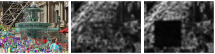
Fig. 1.Example JPEG ghost. Left: a rectangular region has been double-compressed
with primary compression rateq0= 60. Middle and right: in the difference images∆75
and ∆65 a “ghost” gradually appears as a darker region. Note also the noise in ∆75
and∆65due to the image texture.
Iq1,q2. The difference imageDq2 ofIq1 andIq1,q2 is defined as
Dq2(x, y) = 1 3 X i∈{R,G,B} (Iq1(x, y, i)−Iq2(x, y, i)) 2 , (1)
where x and y denote the pixel coordinates, andi ∈ {R, G, B} the red, green and blue color channels.
If a region of the image has previously been compressed with a compression factor q0, q0 < q1, the squared differences become smaller for this part of the
image as q2 approaches q0. This local region, termed “ghost”, appears darker
than the remaining image. This comes from the fact that if the coefficients ofq2
become more similar to the coefficients of (the unknown)q0, similar artifacts are
introduced in the image. For robustness to texture,Dq2(x, y) is averaged across
small windows of sizew. Thus, the differences are computed as
∆q2(x, y) = 1 3w2 X i w−1 X wx=0 w−1 X wy=0 (Iq1(x+wx, y+wy, i)−Iq2(x+wx, y+wy, i)) 2 , (2)
and normalized to lie in the range between 0 and 1.
Fig. 1 shows an example of such a ghost. A rectangular double compressed region has been embedded with q0 = 60 (left). Two difference images∆75 and
∆65 are also shown. The resulting ghost can be clearly seen in ∆65. This can
directly be forensically exploited by examining a number of difference images∆q2
for varyingq2. If a dark region appears, it is considered as doubly compressed.
However, in practice, the amount of human interaction is extremely time-consuming for two reasons. First, one has to closely examine every image, as a ghost can be visually hard to distinguish from noise [2]. Second, the number of difference images can become very large: a ghost appears, if the JPEG grid of∆q2
is exactly aligned with the JPEG grid of the first compression using q0. Thus,
all possible 64 JPEG grid alignments must be visually examined. Ultimately, a human expert has to browse 64·|Q|images, where|Q|is the number of difference images withq2< q1. In practice, there are often more than 300 difference images.
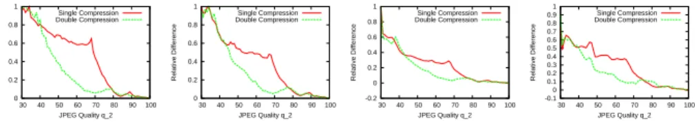
Fig. 2.Difference curves from example JPEG ROIs. The same ROI has been single-and double-compressed single-and is plotted in a joint diagram. In red, the difference curves for single compression are shown, in green for double compression.
3
Feature Extraction
The information about a JPEG ghost is contained in the differences of a single
w×w window over different quality levels. Consider ROIs which have been single- or double-compressed. Example difference curves for this case are shown in Fig. 2. Here, the differences are computed over four different windows of an image with compression qualityq1= 84, over 70 quality levels 30≤q2≤100 on
a window size w= 16. All differences are normalized between 0 and 1. The red curves denote the differences for single compressed windows. The green curves show the same ROIs, but this time double compressed with q0= 69. The green
curve exhibits a second minimum and rapid decay at (the unknown)q0. Due to
differences in image texture, this effect is stronger for the left graphs, than the right graphs.
Our method is based on the analysis of these difference curves. We estimate the quality level q1 as the global minimum over the curves derived from all
windows in the image. We then proceed as follows. Let c(x) be the value of the difference curve for quality levelx. We extracted six features that are defined on
c(x) for 30≤x≤q1. Note that this range implies that we can not detect ghosts
withq0<30. However, this is mainly an engineering decision, as we considered
cases ofq0 <30 as very unlikely. Let, furthermore,w1(x) = (x−30)/(q1−30)
denote a weighting function that puts more emphasis on high JPEG qualities, andw2(x) = 1−w1(x) a weighting function that emphasizes low JPEG qualities.
We employ the following features:
1. The weighted mean value of the curve,
f1= 1 Pq1 x=30w1(x) q1 X x=30 w1(x)·c(x) . (3)
2. The median of all values c(x) for 30≤x≤q1, i. e.f2=µ1/2where
P(c(x)≤µ1/2)≥ 1 2 ∧ P(c(x)≥µ1/2)≥ 1 2 , (4)
andP(c(x)≤x) denotes the cumulative distribution function ofc(x). 3. f3 is the slope of the regression line throughc(x) for 30≤x≤q1.
0 0.2 0.4 0.6 0.8 1 30 40 50 60 70 80 relative difference JPEG quality q2 c(x) lc(x) = 0.5 0 0.2 0.4 0.6 0.8 1 30 40 50 60 70 80 relative difference JPEG quality q2 c(x) regression line 0 0.2 0.4 0.6 0.8 1 30 40 50 60 70 80 relative difference JPEG quality q2 c(x) l(x) l(x) - c(x) 0 0.2 0.4 0.6 0.8 1 30 40 50 60 70 80 relative difference JPEG quality q2 c(x) lc(x) = 0.5 0 0.2 0.4 0.6 0.8 1 30 40 50 60 70 80 relative difference JPEG quality q2 c(x) regression line 0 0.2 0.4 0.6 0.8 1 30 40 50 60 70 80 relative difference JPEG quality q2 c(x) l(x) l(x) - c(x)
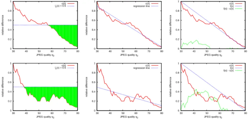
Fig. 3.Visualization of the proposed features. Top: a single-compressed window,
bot-tom: a double-compressed window. Left: area below a normalized error of 0.5. Middle:
regression line on the error curve. Right: squared distance of the curve to the line
between (30,1) and (q1,0).
4. f4is they-axis intercept of the regression line throughc(x) for 30≤x≤q1.
5. The weighted number of points of c(x) withc(x)< t= 0.5,
f5= q1 X x=30 w2(x) −1 · q1 X x=30 w2(x)·g5(x) ,whereg5(x) = 1 if c(x)< t 0 otherwise (5)
6. The average squared distance between the actual curve and the linear func-tionl(x) = 1−(x−30)/(q1−30), i. e. the line connecting (30, 1) and (q1,
0). More formally, f6= q1 X x=30 g6(x) ,whereg6(x) = (l(x)−c(x))2 ifl(x)> c(x) 0 otherwise (6)
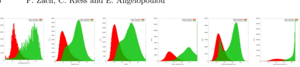
The feature computation is well parallelizable, as every feature depends only on a spatially isolated window. The core idea of this feature set is to identify the steeper decay of the double-compression difference curve (see Fig. 2). Figure 3 illustrates the decision for the feature set on an example window. For each fea-ture, we computed a histogram based on 2.5·106image windows, see Fig. 4. The
compression quality levels of these windows were randomly chosen between 50 and 95, with a fixed distance q0−q1= 20. Feature values of single-compressed
windows are plotted in green, while features of double-compressed windows are shown in red. From left to right, the distributions for f1 to f6 are shown.
Al-though several blocks overlap within a feature, the majority of blocks exhibits good separation between single- and double-compression.
Fig. 4.Histograms of each of the six features,f1,f2, . . . ,f6, shown from left to right.
Red histograms are from double-compressed windows. Green ones correspond to single-compressed windows.
4
Classification
Every block was classified separately, solely based on its features. We evalu-ated different classification algorithms: thresholding, Neural Networks, Random Forests, AdaBoost and Bayes. TheopenCVimplementations of these algorithms were used. The values for thresholding were determined by computing the mean values of the feature distributions for single- and double-compressed areas. The actual threshold was then determined as the mean of means for each feature. A block was considered double-compressed, if at least three quarters of the feature values exceeded their respective threshold. The Neural Network was a Multilayer Perceptron with a 10-node hidden layer. The activation function is a sigmoid function withα=β= 1. For the Random Forests, we used 50 trees for classifi-cation, while for Discrete AdaBoost 100 trees. The cost functions of all classifiers were set to a balanced state of false positive and false negative rates.
5
Experiments
We used the Uncompressed Colour Image Database (UCID) [9] for evaluating our method. It consists of 1338 images of size 512×384. For each image, we created a single-compressed version, and two versions with single- and double-compression, where a randomly chosen 192×192 pixels region is differently compressed than the background. In total, this yields twice as many single- as double-compressed pixels. Per image, we randomly selectedq1∈[50; 95], and set
q0=q1−δ, where 5≤δ≤20. We varied the lengthwof a window between 8 and
64 pixels. Following [5], we excluded very smooth image regions, i. e. windows with an intensity variance below 5 points. For the training of the classifiers, we used 10% of the images from all three classes. Note that the test- and training sets are still weakly correlated due to the high variability of the dataset.
As a quality measure, we used specificity and sensitivity. Let sc and dc denote “single-compressed” and “double-compressed”, respectively. Then, let
TP =P(dc|dc) , TN =P(sc|sc) , FP =P(dc|sc) , FN =P(sc|dc) (7) be the true positives, true negatives, false positives and false negatives, respec-tively. Then, specificity and sensitivity are defined as
specificity = TN
TN + FN , sensitivity = TP
Table 1.Experiments on the UCID database for shifted ghost detection on misaligned DCT grids at a per-window level.
δ w Thresh. MLP RF Boost. Bayes
5 8 0.798/0.702 0.866/0.826 0.804/0.889 0.834/0.886 0.469/0.984 16 0.805/0.704 0.855/0.880 0.811/0.901 0.841/0.893 0.483/0.983 32 0.816/0.717 0.865/0.891 0.838/0.925 0.847/0.919 0.505/0.981 64 0.840/0.596 0.897/0.833 0.889/0.890 0.907/0.870 0.562/0.976 10 8 0.815/0.728 0.865/0.864 0.831/0.901 0.852/0.896 0.479/0.986 16 0.821/0.730 0.869/0.873 0.834/0.914 0.858/0.910 0.497/0.984 32 0.833/0.745 0.835/0.935 0.850/0.941 0.865/0.934 0.520/0.983 64 0.837/0.755 0.917/0.847 0.908/0.893 0.924/0.869 0.579/0.979 20 8 0.844/0.778 0.888/0.910 0.865/0.938 0.895/0.934 0.506/0.985 16 0.849/0.783 0.895/0.906 0.864/0.937 0.902/0.938 0.520/0.984 32 0.857/0.796 0.865/0.935 0.879/0.935 0.912/0.957 0.553/0.983 64 0.861/0.804 0.925/0.892 0.931/0.913 0.938/0.916 0.622/0.977
Note that two other popular measures, the false positive rate and the false neg-ative rate, additively complement specificity and sensitivity to 1. All results in the tables are presented as specificity/sensitivity pairs.
5.1 Experiments on Individual Image Windows
Tab. 1 shows the results for the evaluation perw×wwindow. Here, “Thresh.”, “MLP”, “RF”, “Boost.” and “Bayes” denote classification by thresholding, multi-layer perceptron, random forests, discrete AdaBoost and the Bayesian classifier, respectively. The difference in the quality levels of primary and secondary com-pression is denoted asδ=q1−q0. In order to have a relatively balanced number
of single and double compressed pixels, we only evaluated the performance on the correct shift of the doubly-compressed region. However, when we evaluated the whole pipeline, we tested all 64 shifts of the JPEG grid.
The best performance per classifer (considering the sum of specificity and sensitivity) on all combinations of δand the region size is printed in italics. As expected, typically the highest tested compression distance of δ= 20, together with the largest examined window size 64×64 yields best results. Note that AdaBoost performed best below the maximum windows size. Note also that for
δ = 10 and δ = 5, boosting, followed by neural networks (MLP) and random forests (RF) all provide very strong results. Furthermore, the performance of these three methods degrades gracefully for smaller windows. Thus, as a pre-processing step for guiding a human expert towards a JPEG ghost location, we consider these three classifiers highly suitable. Additionally, the good discrimina-tion for small values ofδimproves over the results reported in [5], which reports
δ≥20 as a good quality distance for detection. In [7], detection rates forδ≤10 vary between 50% and 70%.
32 - 0.812/0.755 0.749/0.889 0.726/0.949 0.811/0.883 0.742/0.822 64 - 0.830/0.481 0.963/0.355 0.978/0.375 0.982/0.378 0.882/0.606 10 8 0.658/0.597 0.820/0.759 0.774/0.874 0.913/0.857 0.918/0.880 0.594/0.892 16 - 0.827/0.758 0.777/0.870 0.897/0.873 0.916/0.899 0.772/0.815 32 - 0.830/0.737 0.776/0.857 0.882/0.883 0.916/0.895 0.840/0.845 64 - 0.852/0.439 0.946/0.377 0.968/0.416 0.989/0.412 0.938/0.684 20 8 0.705/0.605 0.832/0.880 0.864/0.941 0.905/0.960 0.997/0.939 0.533/0.997 16 - 0.858/0.883 0.892/0.957 0.904/0.973 0.996/0.956 0.647/0.997 32 - 0.867/0.868 0.865/0.947 0.908/0.972 0.993/0.960 0.839/0.988 64 - 0.933/0.484 0.866/0.517 0.959/0.519 0.997/0.507 0.960/0.955
5.2 Experiments on Automated Tampered Image Detection
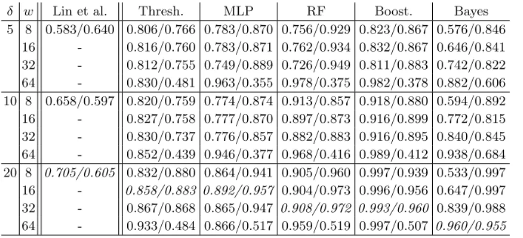
For comparison to other methods, we implemented a straightforward tampered image classifier based on the recognition of partially double-compressed JPEG images. To remove outliers on the marked windows from the previous section, we applied a 3×3 pixels morphological opening with a cross-topology on these markings. We considered an image tampered, if 10% of the windows are marked. Note that an embedded foreground-ghost contains about 20% double-compressed pixels, a background-ghost about 100%−20% = 80%. As before, we created three images from every UCID image. Once completely single-compressed, once with an embedded foreground-ghost, and once with an embedded background-ghost. Tab. 2 shows the result for JPEG ghosts that were exactly aligned with the JPEG grid. We used the same notation as in the previous Subsection.
For comparison, we evaluated the method of Lin et al. [7] on our test set. As this method operates on 8×8 windows, only these results are presented. The approach of Lin et al. is more general, in the sense that it can also detect double-compression where q0 > q1. However, this comes at the expense of the
accuracy in the presence of very small differences in the compression parameters. Thus, if the initial assumptionq0< q1for JPEG ghosts is fulfilled, the proposed
method provides much higher specificity and sensitivity rates.
The best success rates do not occur at the larger window sizes. This is due to the fact that the embedded foreground ghosts of 192×192 pixels are com-parably small. When applying morphological opening on the windows that have been marked as double-compressed, more accurate detectors lose too many win-dows on the boundary of the marked region. This renders very large window sizes less successful. One notable exception is the Bayesian classifier. As can be seen from Tab. 1, Bayesian classification exhibits very low specificity, i. e. creates many erroneously marked regions. The morphological operator removes a large
Table 3. Experiments on UCID database for shifted ghost detection on misaligned DCT grids on image level.
δ w Thresh. MLP RF Boost. Bayes
5 8 0.742/0.772 0.982/0.904 0.923/0.960 0.990/0.955 0.907/0.981 16 0.755/0.708 0.993/0.934 0.940/0.952 0.987/0.944 0.919/0.982 32 0.750/0.698 0.973/0.915 0.969/0.952 0.984/0.947 0.923/0.983 64 0.763/0.468 0.967/0.765 0.992/0.843 1.000/0.809 0.951/0.983 10 8 0.762/0.794 0.978/0.932 0.938/0.957 0.978/0.951 0.923/0.983 16 0.779/0.733 0.975/0.913 0.955/0.954 0.984/0.948 0.945/0.983 32 0.791/0.728 0.981/0.968 0.961/0.957 0.986/0.950 0.951/0.983 64 0.795/0.646 0.984/0.755 0.993/0.803 0.998/0.775 0.966/0.986 20 8 0.784/0.836 0.977/0.955 0.969/0.972 0.993/0.971 0.987/0.985 16 0.802/0.795 0.963/0.939 0.978/0.972 0.995/0.969 0.993/0.987 32 0.806/0.786 0.862/0.953 0.948/0.963 0.995/0.971 0.995/0.988 64 0.810/0.659 0.988/0.833 0.994/0.806 0.999/0.818 0.997/0.988
Fig. 5.Two example markings on individual windows. Green and red are single- and double compressed, respectively. Gray denotes low contrast regions. Left: the rectan-gular double compression region could only in the high-contrast windows be recovered. Right: the double compression region is clearly visible. In a classification on image level, the left example is a false negative case, the right example true positive.
number of these false positive markings, and makes detection with larger win-dow sizes possible. In comparison, the remaining classifiers exhibit their peak performance at window sizes around 16×16 pixels. Again, discrete Adaboost clearly outperforms the other methods.
In shifted double-compression, the grid of the inserted region is not required to properly align with the JPEG grid of the background. To detect such tampered images, we computed all 64 shifts and selected the one with the highest response of double-compressed blocks (see Tab. 3 for the results). A surprising result is that shifted double JPEG compression can be slightly better discriminated than the non-shifted version: while the overall best result in Tab. 2 is 0.997/0.939, several results in Tab. 3 perform better, e. g. the Bayesian classifier on a 64×64 grid for δ= 20 with 0.997/0.988. During shifted double-compression,q1 = 100
is often (wrongly) estimated. Interestingly, the increased gap betweenq0 andq1
6
Conclusions
We proposed a JPEG-based forensic algorithm to automatically distinguish single-compressed and double-compressed image regions. We presented a clas-sification scheme that exploits the JPEG-ghost effect, but completely removes the requirement of browsing the images. Best results were achieved by training a boosted classifier on 6 specially designed features. The classification perfor-mance is encouraging. The best specificity and sensitivity are 0.912 and 0.957, respectively. For tampering detection, the difference in primary and secondary compression may be as small asδ= 5.
References
1. Barni, M., Costanzo, A., Sabatini, L.: Identification of Cut & Paste Tampering by Means of Double-JPEG Detection and Image Segmentation. In: International Symposium on Circuits and Systems. pp. 1687–1690 (May 2010)
2. Battiato, S., Messina, G.: Digital Forgery Estimation into DCT Domain — A Critical Analysis. In: Multimedia in Forensics, Security and Intelligence. pp. 37–42 (Oct 2009)
3. Bayram, S., Sencar, H.T., Memon, N.: A survey of copy-move forgery detection techniques. In: IEEE Western New York Image Processing Workshop (2009) 4. Farid, H.: A Survey of Image Forgery Detection. Signal Processing Magazine 26(2),
16–25 (Mar 2009)
5. Farid, H.: Exposing Digital Forgeries from JPEG Ghosts. IEEE Transactions on Information Forensics and Security 1(4), 154–160 (2009)
6. Huang, F., Huang, J., Shi, Y.Q.: Detecting Double JPEG Compression With the Same Quantization Matrix. IEEE Transactions on Information Forensics and Se-curity 5(4), 848–856 (Dec 2010)
7. Lin, Z., He, J., Tang, X., Tang, C.K.: Fast, Automatic and Fine-grained Tampered JPEG Image Detection via DCT Coefficient Analysis. Pattern Recognition 52(11), 2492–2501 (Nov 2009)
8. Qu, Z., Luo, W., Huang, J.: A Convolutive Mixing Model for Shifted Double JPEG Compression with Application to Passive Image Authentication. In: International Conference on Acoustics, Speech and Signal Processing. pp. 1661–1664 (Mar 2008) 9. Schaefer, G., Stich, M.: UCID - An Uncompressed Colour Image Database. In: SPIE Storage and Retrieval Methods and Applications for Multimedia. pp. 472– 480 (Jan 2004)
10. Sencar, H., Memon, N.: Overview of State-of-the-art in Digital Image Forensics. Algorithms, Architectures and Information Systems Security pp. 325–344 (2008)