Development of Construction Projects Scheduling with Evolutionary Algorithms
Mehdi Tavakolan
Submitted in partial fulfillment of the
Requirements for the degree of
Doctor of Philosophy
in the Graduate School of Arts and Sciences
COLUMBIA UNIVERSITY
2011
© 2011 Mehdi Tavakolan All rights reserved
ABSTRACT
Development of Construction Projects Scheduling with Evolutionary Algorithms Mehdi Tavakolan
Evolutionary Algorithms (EAs) as appropriate tools to optimize multi-objective problems have
been applied to optimize construction projects in the last two decades. However, studies on
improving the convergence ratio and processing time in the most applied algorithms such as
Genetic Algorithm (GA), Particle Swarm Optimization (PSO) and Ant Colony Optimization
(ACO) in construction engineering and management domains remain poorly understood.
Furthermore, hybrid algorithms such as Hybrid Genetic Algorithm-Particle Swarm Optimization
(HGAPSO) and Shuffled Frog Leaping Algorithm (SFLA) have been presented in computational
optimization and water resource management domains during recent years to prevent pitfalls of
the aforementioned algorithms. In this dissertation, I present three studies on hybrid algorithms
to show that our proposed hybrid approaches are superior than existing optimization algorithms
in finding better project schedule solutions with less total project cost, shorter total project
duration, and less total resources allocation moments. In the first, I present a HGAPSO approach
to solve complex, TCRO problems in construction project planning. Our proposed approach uses
the fuzzy set theory to characterize uncertainty about the input data (i.e., time, cost, and
resources required to perform an activity). In the second, I present the SFLA algorithm to solve
TCRO problems using splitting allowed during activities execution. The third study involves the
evaluation of the inflation impact on resources unit price during execution of construction
projects. This research presents the comprehensive TCRO model by comparing two hybrid
six different examples in terms of the structure of projects, construction assumptions and kinds
of Time-Cost functions. Each of the three studies helps overcome parts of EAs problems and
contributes to obtaining optimal project schedule solutions of total project duration, total project
cost and total resources allocation moments of construction projects in the planning stage. The
ii
TABLE OF CONTENTS
Chapter 1. Introduction and Background………...…1
1.1 Genetic Algorithm (GA)………..……….…3
1.2 Particle Swarm Optimization (PSO) …….……….……..4
1.3 Ant Colony Optimization (ACO) ……...………..………7
1.4 Hybrid Genetic Algorithm- Particle Swarm Optimization (HGAPSO)…………...12
1.5 Shuffled Frog Leaping Algorithm (SFLA)..…..………...13
1.6 Constraints of the Current Methodology………..………...13
1.7 Format and Flow of this Dissertation………..………14
Chapter 2. Time-Cost-Resource Optimization in Construction Project Planning: A Fuzzy Enabled Hybrid Genetic Algorithm-Particle Swarm Optimization (HGAPSO) Approach………..17
Abstract………...………...17
2.1 Introduction….…………..………...…18
2.2 Research Background…….………..………...…………19
2.3 Mathematical Formulation of a Time-Cost-Resource Optimization (TCRO) Problem in Construction Project Planning.………...…...…23
2.4 Fuzzy Enabled Hybrid Genetic Algorithm-Particle Swarm Optimization (HGAPSO) Algorithm.………...…...25 2.5 Application of the Proposed Fuzzy Enabled HGAPSO Algorithm…...………..30 i
iii 2.5.1 Example 2.1 ……….30 2.5.2 Example 2.2……….………...…….….36 2.5.3 Example 2.3………..41 2.6 Discussion………...……….45 2.7 Conclusions..……….………..…….46
Chapter 3. Applying the Shuffled Frog-Leaping Algorithm to Time-Cost-Resource Optimization Problems with Activity Splitting Allowed………..………....49
Abstract………...……….………..………....49
3.1 Introduction……….……….50
3.2 Research Background……….………...……….….51
3.3 Mathematical Formulation of Time-Cost-Resource Optimization (TCRO) Problems with Activity Splitting Allowed in Construction Project Planning……...54
3.3.1 Objective Functions…….………..………...57
3.3.2 Constraints of the Model………….………..58
3.4 Shuffled Frog Leaping Algorithm (SFLA) Algorithm to Solve TCRO Problems in Construction Project Planning…………...……….………...…...……….60
3.5 Application of the Proposed SFLA Algorithm.………...…...……….65
3.5.1 Example 3.1…….………...……...………….…………..65
3.5.2 Example 3.2…….………...………..73
iv
Chapter 4. Comparison of Evolutionary Algorithms in Non-dominated Solutions of
Time-Cost-Resource Optimization Problems with Evaluation of Inflation Impact….……...…..84
Abstract………...………...….………84
4.1 Introduction….……….85
4.2 Research Background…….………...…………...…….88
4.3 Computation of Inflation.………...……….……….……91
4.4 Application of the Proposed Hybrid Algorithms with Inflation rate of Resources Unit Price ………...………..….91
4.4.1 Example 4.1……….………...……...………….………..92
4.4.2 Example 4.2………….…………..………...……..103
4.5 Comparison of Significant Parameters of Evolutionary Algorithms.…………...….114
4.6 Conclusions…….…………...………..……...…..115
Chapter 5. Conclusions and Future Works………..…………...117
v
LIST OF FIGURES
Figure 1.1 Schematic of PSO Algorithm………...………7
Figure 1.2 Schematic of ACO algorithm………...…………..………8
Figure 1.3 The flowchart of the ACO Algorithm………...……….…...…..….10
Figure 2.1 Flowchart of the proposed TCRO model………...…..……23
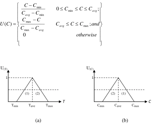
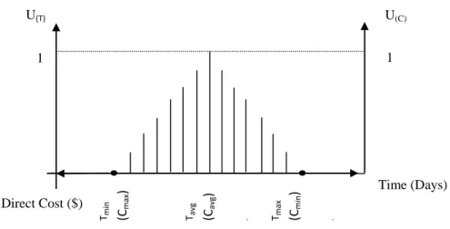
Figure 2.2 Fuzzy membership function for duration (a) and direct cost (b) of activities….…….27
Figure 2.3 An overview of our proposed HGAPSO algorithm….….…………...………29
Figure 2.4 AON diagram of project activities in Example 2.1….………...…..31
Figure 2.5 Discretized membership functions for duration and direct cost of activities………...31
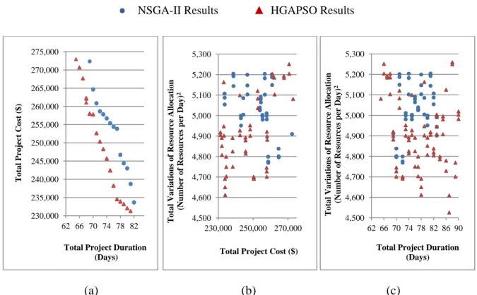
Figure 2.6 Optimal project schedule solutions in the 2-dimensional space of total project cost and total project duration found by our proposed HGAPSO, and Zahraie and Tavakolan’s algorithms in Example 2.1……….………...……...………33
Figure 2.7 Optimal project schedule solutions in the 3-dimensional space of total project cost, total project duration and total variations of resource allocation found by (a) NSGA-II approach; and (b) our proposed HGAPSO algorithm in Example 2.1……..………….……….…...34
Figure 2.8 Optimal project schedule solutions in the 2-dimensional space of (a) total project cost and total project duration; (b) total project cost and total variations of resource allocation; and (c) total project duration and total variations of resource allocation found by the NSGA-II approach and our proposed HGAPSO algorithm in Example 2.1……….35
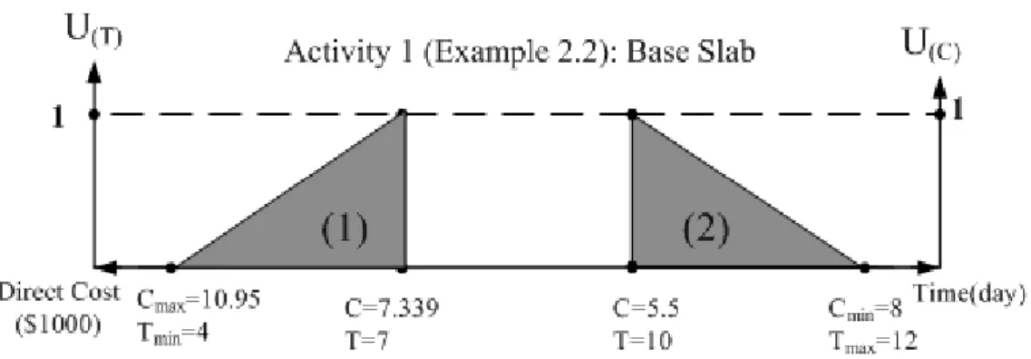
Figure 2.9 AON diagram of project activities in Example 2.2.………...…..36
Figure 2.10 Continuous membership functions for duration and direct cost of activities……...37
Figure 2.11 Optimal project schedule solutions in the 2-dimensional space of total project cost and total project duration by our proposed HGAPSO algorithm, and Zahraie and Tavakolan’s NSGA-II algorithm in Example 2.2………...………40
vi
Figure 2.12 Optimal project schedule solutions in the 3-dimensional space of total project cost, total project duration and total variations of resource allocation found by (a) NSGA-II approach;
and (b) our proposed HGAPSO algorithm in Example 2.2………...41
Figure 2.13 Optimal project schedule solutions in the 2-dimensional space of (a) total project cost and total project duration; (b) total project cost and total variations of resource allocation; and (c) total project duration and total variations of resource allocation found by the NSGA-II approach and our proposed HGAPSO algorithm in Example 2.2……….…....42
Figure 2.14 AOA diagram of project activities in Example 2.3….………...…43
Figure 2.15 Optimal project schedule solutions in the 2-dimensional space of total project cost and total project duration by our proposed HGAPSO algorithm in Example 2.3………...………44
Figure 2.16 Optimal project schedule solutions in the 3-dimensional space of total project cost, total project duration and total variations of resource allocation found by our proposed HGAPSO algorithm in Example 2.3………...…45
Figure 3.1 Occupying positions of activity i based on ESi (without Splitting)…..………….…55
Figure 3.2 Occupying positions of activity i (with splitting).……….……...…..….…56
Figure 3.3 Example of a relationship constraint.………. ……….……59
Figure 3.4 The memeplex partitioning process.………....….…………..…..61
Figure 3.5 The flowchart of the SFLA algorithm.….………... ………64
Figure 3.6 Optimal project schedule solutions in the 2-dimensional space of total project cost and total project duration found by our proposed SFLA algorithm (before and after splitting allowed), and Zahraie and Tavakolan’s algorithms in Example 3.1.……….……67
Figure 3.7 Optimal project schedule solutions in the 3-dimensional space of total project cost, total project duration and total variations of resource allocation found by (a) NSGA-II approach; and (b) our proposed SFLA algorithm before splitting allowed; and (c) our proposed SFLA algorithm after splitting allowed in Example 3.1………...….…...………69
Figure 3.8 Optimal project schedule solutions in the 3-dimensional space of total project cost, total project duration and total time utilizations of resource allocation found by (a) NSGA-II approach; and (b) our proposed SFLA algorithm before splitting allowed; and (c) our proposed SFLA algorithm after splitting allowed in Example 3.1………..…..70
vii
Figure 3.9 Optimal project schedule solutions found by the NSGA-II approach and our proposed SFLA algorithm (before and after splitting allowed) in the 2-dimensional space of total project cost and total project duration; (a) in space of total variations of resource allocation; and (b) in space of total time utilizations of resource allocation in Example 3.1………..71 Figure 3.10 Optimal project schedule solutions found by the NSGA-II approach and our proposed SFLA algorithm (before and after splitting allowed) in the 2-dimensional space of (a) total project duration and total variations of resource allocation; (b) and total project duration and total time utilizations of resource allocation in Example 3.1……….72 Figure 3.11 Optimal project schedule solutions found by the NSGA-II approach and our proposed SFLA algorithm (before and after splitting allowed) in the 2-dimensional space of (a) total project cost and total variations of resource allocation; (b) and total project cost and total time utilizations of resource allocation in Example 3.1………..….……..72 Figure 3.12 Activity on Node (AON) Network of Example 3.2………...74
Figure 3.13 Optimal project schedule solutions in the 2-dimensional space of total project cost and total project duration found by our proposed SFLA algorithm before and after splitting allowed in Example 3.2………..…………..…...…….77 Figure 3.14 Optimal project schedule solutions in the 3-dimensional space of total project cost, total project duration and total variations of resource allocation found by (a) our proposed SFLA algorithm before splitting allowed; and (b) our proposed SFLA algorithm after splitting allowed in Example 3.2………...………...……….78 Figure 3.15 Optimal project schedule solutions in the 3-dimensional space of total project cost, total project duration and total time utilizations of resource allocation found by (a) our proposed SFLA algorithm before splitting allowed; and (b) our proposed SFLA algorithm after splitting allowed in Example 3.2……….………...………..79 Figure 3.16 Optimal project schedule solutions found by the NSGA-II approach and our proposed SFLA algorithm (before and after splitting allowed) in the 2-dimensional space of total project cost and total project duration; (a) in space of total variations of resource allocation; and (b) in space of total time utilizations of resource allocation in Example 3.2………..…….……..80 Figure 3.17 Optimal project schedule solutions found our proposed SFLA algorithm (before and after splitting allowed) in the 2-dimensional space of (a) total project duration and total variations of resource allocation; (b) and total project duration and total time utilizations of resource allocation in Example 3.2………...…..…….81 Figure 3.18 Optimal project schedule solutions found by our proposed SFLA algorithm (before and after splitting allowed) in the 2-dimensional space of (a) total project cost and total variations of resource allocation; (b) and total project cost and total time utilizations of resource allocation in Example 3.2………..………81 Figure 4.1 The evolution process of three EAs (GA, PSO, ACO)………..…..89
viii
Figure 4.2 Activity on Node (AON) Network of Example 4.1………..…...93
Figure 4.3 Optimal project schedule solutions before applying inflation in the 2-dimensional space of total project cost and total project duration found by our proposed hybrid algorithms, our proposed GA and PSO in Example 4.1……….….….96 Figure 4.4 Optimal project schedule solutions after applying inflation in the 2-dimensional space of total project cost and total project duration found by our proposed hybrid algorithms, and our proposed GA and PSO in Example 4.1……….…….97 Figure 4.5 Optimal project schedule solutions found by the (a) NSGA-II, (b) PSO, (c) SFLA, and (d) HGAPSO algorithms after applying inflation in the 3-dimensional space of total project cost, total project duration and total resource allocation (Z3) in Example 4.1………...………..99 Figure 4.6 Optimal project schedule solutions found by the (a) NSGA-II, (b) PSO, (c) SFLA, and (d) HGAPSO algorithms after applying inflation in the 3-dimensional space of total project cost, total project duration and total resource allocation (Z4) in Example 4.1………..….……100
Figure 4.7 Optimal project schedule solutions found by the (a) NSGA-II, (b) PSO, (c) SFLA, and (d) HGAPSO algorithms after applying inflation in the 3-dimensional space of total project cost, total project duration and total resource allocation (Z5) in Example 4.1………...…101 Figure 4.8 Optimal project schedule solutions found by the NSGA-II, PSO, SFLA, and HGAPSO algorithms (after applying inflation) in the 2-dimensional space of total project cost and total project duration; (a) in space of total variations of resource allocation; and (b) in space of total time utilizations of resource allocation; and (c) in resource allocation space; (d) total project duration and total variations of resource allocation; (e) and total project duration and total time utilizations of resource allocation; and (f) total project duration and total resources allocation; (g) total project cost and total variations of resource allocation; (h) and total project cost and total time utilizations of resource allocation; and (i) total project cost and total resources allocation in Example 4.1………...……….…103 Figure 4.9 Activity On Arrow (AOA) Network of Example 4.2...………...105
Figure 4.10 Optimal project schedule solutions found by the NSGA-II, PSO, SFLA, and HGAPSO algorithms in the 2-dimensional space of total project cost and total project duration, (a) before applying inflation, and (b) after applying inflation with indirect cost= $1,500 in Example
4.2……….………..…..107 Figure 4.11 Optimal project schedule solutions found by the (a) NSGA-II, (b) PSO, (c) ACO, (d) SFLA, and (e) HGAPSO algorithms after applying inflation in the 3-dimensional space of total project cost, total project duration and total variations of resources allocation (Z3) with indirect cost= $1,500 in Example 4.2 ……….………...………..110
ix
Figure 4.12 Optimal project schedule solutions found by the (a) NSGA-II, (b) PSO, (c) ACO, (d) SFLA, and (e) HGAPSO algorithms after applying inflation in the 3-dimensional space of total project cost, total project duration and total time utilizations of resource allocation (Z4) with indirect cost= $1,500 in Example 4.2………..………111 Figure 4.13 Optimal project schedule solutions found by the (a) NSGA-II, (b) PSO, (c) ACO, (d) SFLA, and (e) HGAPSO algorithms after applying inflation in the 3-dimensional space of total project cost, total project duration and total resource allocation (Z5) with indirect cost= $1,500 in Example 4.2……….………...……..…...112
x
LIST OF TABLES
Table 1.1 Selected important studies of time-cost tradeoff concepts with application of
Evolutionary Algorithms……….…… ………...…...…11
Table 1.2 Selected important studies of resource management concepts with application of Evolutionary Algorithms.………...……….……....12
Table 2.1 Feasible project schedule options to perform Activity 1 in Example 2.1…….…...…..33
Table 2.2 Cost-Time functions to perform project activities in Example 2.2………….….……..38
Table 2.3 Examples of feasible project schedule options to perform Activity 1 in Example 2.2..39
Table 2.4 Feasible project schedule options to perform project activities in Example 2.3….…..43
Table 2.5 Comparison of processing time (in minutes) to solve Examples 2.1 and 2.2 using our proposed Hybrid Genetic Algorithm-Particle Swarm Optimization approach and existing optimization algorithms………...………..46
Table 3.1 Details of Example 3.1……….………..66
Table 3.2 The fixing unit price of resources in Example 3.2……….75
Table 3.3 Different options for the first activity in Example 3.2…….…...………...…75
Table 3.4 The detailed information of activities in Example 3.2………….………..76
Table 4.1 Recent Values of Inflation of Resources (ENR)…….………...87
Table 4.2 Details of Calculation of Inflation Rate…….………91
Table 4.3 Details of Example 4.1……….………..94
xi
Table 4.5 Feasible project schedule options to perform Activity 1 in Example 4.2….……...…106
Table 4.6 The increases of cost solutions when indirect cost= $3,000 against $1,500 in Example 4.2………...…..………113 Table 4.7 The comparison of required iteration numbers by Evolutionary Algorithms in Examples: 4.1, and 4.2….……...…………..………...……114 Table 4.8 The values of significant parameters of EAs in both Examples………...…...115
xii
ACKNOWLEDGMENTS
First of all I am deeply grateful to Professor Raimondo Betti for all his great recommendations
and financial support during my last year of Ph.D. experience. He has also been very dedicated,
helpful, and considerate mentor for me. I would also like to express my respectful gratitude to
my principle co-advisor Professor Baabak Ashuri for all his great recommendations to complete
this research. Without him, the accomplishment of these papers would otherwise have remained
a castle in the air.
Thanks are also extended to the rest of defense committee, Professor Rene B. Testa,
Professor Soulaymane Kachani, and Professor Andrew W. Smyth for reviewing this dissertation
and giving precious advice.
Sincere thanks also go to Professor Nicola Chiara for his great support during my first year
at Columbia University. I also gratefully acknowledge all great recommendations of Professor
Tehranizadeh who motivated me and helped me endure the sometimes frustrating obstacle that
arises in the pursuit of a Ph.D.
On the personal side, I want to thank my father, my mother, my wife’s parent, and my
brothers for all their great support. I have no word to express my sincere appreciation and love
for all that to my wife, Setareh, gave up to make this research possible. Furthermore, I would like
to express my gratitude to my aunt, Mrs. Monir Almassi, and her husband, Dr. Hossein Almassi
for all their great support. I also want to thank Mrs. Negin Almassi for her editing help.
Mehdi Tavakolan
xiii
Dedicated
To
My Respected Father, Mohammadhadi,
My Beloved Mother, Batool,
And
Chapter 1
Introduction and Background
Time, cost and resource management are three dimensions of project management in
concepts of project control (PMBOK 2008). The Critical Path Method (Abraham et al. 1998;
Shi et al. 2000; Lu and AbouRizk 2000; Galloway et al. 2006; Ibbs et al. 2007; and
El-Rayes et al. 2009), Program Evaluation and Review Technique (Cottrell et al. 1999;
AbouRizk et al. 2000; Lu et al. 2002 and; and Lee et al. 2006), and Graphical Evaluation and
Review Technique (Pena-Mora and Park 2001) are three seminal methods for controlling the
structure of projects including activities with various durations and budgets.
In the last two decades, much effort has focused on the optimization of scheduling by
considering the impact of various activities of construction projects. Time-Cost Optimization
(TCO), resource leveling, and resource allocation are the three most important problems that
have been evaluated in construction engineering and management concepts. The increasing
acceptance of different project delivery systems allows greater flexibility in construction
duration, to the mutual benefit of both client and contractor. This also means that both
construction time and cost should be considered concomitantly in the estimation and planning
stages (Zheng et al. 2005). TCO is a process used to identify suitable construction activities for speeding up, and for deciding “by how much” so as to attain the best possible savings in both total duration and cost of projects (Zheng and Ng 2005). Resource allocation is used to
assign available resources in an economic way or to schedule activities and the resources
the project time (PMBOK 2008). In addition, resource leveling is a project management
process used to examine unbalanced use of resources over time, and for resolving
over-allocations or conflicts (PMBOK 2008). However, the increase of project control importance
in construction project makes it such that clients, contractors, and sponsors seek to improve
their estimates and forecasting evaluations of project problems in the planning stage.
Software packages such as Microsoft Project and Primavera and searching tools such as
mathematical programming, heuristic models and evolutionary algorithms have been
extensively applied to optimize the scheduling of construction projects. However, most of the
construction projects scheduling software packages do not have the capability to set a
limitation on resources for each activity over the duration of the project (Kim and Ellis 2010).
Furthermore, the difficulties associated with using mathematical optimization on large-scale
engineering problems have contributed to the development of alternative solutions (Elbeltagi
et al. 2005). In addition, heuristic models quite possibly could provide good solutions, but do
not guarantee optimality (Hegazy 1999). Since Evolutionary Algorithms (EAs) have greater
capabilities in optimizing complex problems with widespread solutions, we apply EAs to
construction problems. The main motivation for using EAs to solve multi-objective
optimization problems is due to its capability for searching simultaneously with a set of
possible solutions to find the optimal Pareto front with a fewest runs of algorithm. Moreover,
EAs are less susceptible to the shape or continuity of the Pareto front (Coello Coello 2002).
EAs can be applied as multi-objective optimization tools to obtain the most appropriate
solutions. In multi-objective problems, the decision maker is required to select a solution
from a Pareto front solution by making compromises, which provide for acceptable
performance over all objectives (Lamont et al. 2002). Cohon and Marks (1975) classified
multi-objective methods in three categories: generating techniques with a posteriori
techniques which rely on progressive articulation of preferences. Genetic Algorithm (GA),
Particle Swarm Optimization (PSO), and Ant Colony Optimization (ACO) have been
extensively applied in optimization of construction problems. We briefly describe the
algorithms in the following Sections:
1.1 Genetic Algorithm (GA)
As the first introduced evolutionary algorithm, GA has been used widely in various aspects of
engineering problems such as constrained or unconstrained optimization, scheduling and
reliability optimization. GA is a searching and optimization tool based on natural evolution. It
directs the initial population toward the global optimum points according to the objective
function. This method is presented by John Holland in 1997 and then developed by one of his
students, David Goldberg, in 1989 for solving problems in controlling gas piping line
transfers. A solution to a given problem is represented in the form of a string, called
chromosome, consisting of a set of elements called genes that hold a set of values for the
optimization variables (Goldberg 1989). In general, GA includes four important steps: (1)
Generation of an initial population; (2) selection of the best chromosomes based on their
fitness value; (3) crossover of the old chromosome to produce new chromosome in the next
generation; (4) mutation of new chromosomes to extend the scope of searching. Usually some
of the best chromosomes called an elitism genes go directly to the next generation. Based on
the GA process, four important parameters including population size, Pcrossover ,Pmutation and
size of crowding distance have significant impact on the convergence ratio and quality of
Pareto front solution (Goldberg 1989; Konak et al. 2006). Figure 1.1 shows GA optimization
processes.
Some multi-objective algorithms initially have been applied to genetic algorithms.
method of genetic algorithm to optimize Pareto front with non-dominated solutions. Hajela
and Lin (1992) introduce Weighted Based Genetic Algorithm (WBGA) with normalization of
objective functions. Coello and Montes (2004) suggest the Niched Pareto Genetic Algorithm
(NPGA) and Lu and Yen (2003) propose the Pareto Evolutionary Selective Algorithm
(PESA) as genetic algorithms developed. Based on Deb’s research (2000), each of the
mentioned algorithms is suitable for the specific case studies; meanwhile, they have related
problems in convergence speed to the final solution. However, the most applied
multi-objective algorithm is the Non-dominated Sorting Genetic Algorithm (NSGA). The NSGA
algorithm is first suggested by Goldberg (1989) and then implemented by Srinivas and Deb
(1994). This algorithm uses the crowding technique to ensure diversity among non-dominated
solutions. This method is computationally efficient and is capable of finding a good spread of
Pareto optimal solutions (Deb et al. 2000). El-Rayes et al. (2006) improve multi-objective
genetic algorithms to optimize resource utilization in large-scale construction projects.
GA has several limitations. Fogel (1995) present some deficiencies in GA performance,
including premature convergence or a slow convergence process (requiring a large number of
generations) have been also identified. Ng and Zheng (2008) state that despite the benefit of
GA, the time taken by a GA model to generate a near-optimum solution can be excessive.
Another major drawback of GAs has to do with genetic drift which is typified by the
existence of multiple peaks of equal height. When genetic drift occurs, it will converge to a
single peak due to stochastic errors during processing, which is undesirable for any
multi-objective problems (Zheng et al. 2005).
1.2Particle Swarm Optimization (PSO)
In comparison with GA, Particle Swarm Optimization (PSO) is a newer algorithm which is
of flight of a flock of birds. A large number of birds flock synchronously, change direction
suddenly, and scatter and regroup together (Yin et al. 2005). Each particle adjust its flying
from the experience of its own and that of the other members of the swarm during the search
for food (Yin et al. 2005). Like the evolutionary algorithm, PSO search operates through
updating swarms (population) of particle. There are some similarities between PSO and GA
(Grosan et al 2005):
Both techniques use a population of solutions from the search space which are initially randomly generated;
Solutions belonging to the same population interact with each other during the search process;
Solutions are evolved (their quality is improved) using techniques inspired from the real world.
On the basis of classical PSO, the algorithm maintains an elite set of non-dominated
solutions and redefines the selections of guides during the optimization process (Yang 2007).
In contrast to GA, PSO has the advantage of keeping the continuity between individuals to
converge faster although it may easily get into the local optimum (Shahgholi et al 2006). In
PSO, each particle corresponds to a candidate solution of the underlying problem. Unlike a
GA that reproduces chromosomes of the next generation from unclassified survivals, PSO
updates a population of particles with the internal velocity and attempts to profit from the
discoveries of themselves and previous experiences of other companions.
In PSO, a population of particles is randomly initialized with position and velocities. A
particle i is treated as a point in a multi-dimensional space
j
and status of the particle is characterized by its position and velocity (Kennedy and Eberhart 1995). During each PSOdimension
j
by referring to, with random multipliers, the personal best vector(
pbest
ij)
and the swarm’s best vector(
gbest
j)
. The updated functions for particle flying can be formulated as (Eberhart and Shi 1998):)) ( ) ( ( )) ( ) ( ( ) ( ) 1
(t v t c1r1 pbest t particle t c2r2 gbest t particle t
vij iteration ij ij ij j ij (1.1) ) 1 ( ) 1 ( ) ( ) 1 (t particle t v t t when t particle ij ij iteration ij (1.2)
where
is inertia coefficient, which has an important role in balancing a global (a large value of
) and local search (a small value of
);c
1 andc
2 are the cognitive coefficients ;1
r
andr
2 are the uniform random real numbers in (0,1), and the symbol iteration is used to show the updated values from iterationt
to next iterationt
1
. The parameters that have the most considerable impact on the convergence ratio and Pareto front arec
1,c
2 and
. The inertia weight
can be constant or varying with iteration. Varying inertia weight (from larger to smaller) use to be recommended to enhance global exploration for early iterationsand to facilitate local exploration for last iterations (Zhang et al. 2006).
The basic PSO algorithm consists of three steps: generating particles’ positions and
velocities, velocity updating and position updating. Equation (1,1) is used to calculate a
particle’s new velocity according to its previous velocity and the distances of its current
position from its local best and the global best. Equation (1,2) is used to calculate the new
position of a particle by utilizing its previous experience (i.e., local best) and the experience
for all particles (i.e., global best). These two equations also reflect the unique mechanism of
operator PSO (Zhang et al. 2006).
The selection of pbest(t)simply replaces the previous best experience by the current position if the former does not strongly dominate the latter. The selection of gbest(t) is
altered to promote population diversity without overlooking the edges and sparse areas (Yang
2007). Figure 1.1 shows the PSO concept in a 3D search space. Particle 1 moves to new
position based on previous best experience (particle 6) and the best among the swarm
(particle 5). In multi-objective PSO, multiple non-dominated solutions are usually sought.
The main difference in the multi-objective approach is how the pbestandgbestvectors are defined (fitness evaluation), and given that these vectors are not unique anymore, what values
of pbest and gbest are selected to be used in equation (1.1) are important (Baltar et al.
2008). 1 2 3 5 4 6 pbest(t) particle (t) V(t+1) gbest(t) particle (t+1)
Figure 1.1 Schematic of the PSO Algorithm
1.3Ant Colony Optimization (ACO)
Ant Colony Optimization (ACO) is proposed by Colorni (1991), which Dorigo and Maniezzo
(1997) apply to travelling sales problems. Similar to PSO, ACO algorithm evolves not in
their genetics but in their social behavior. As Figure 1.2 shows, ants can find the shortest path
from their nest to food by laying pheromones on the ground as they move. The pheromone
dissipates over time but it is strengthened when other ants travel on the same trail again.
Those arriving subsequently choose the trails with denser pheromones, and they further
eventually be abandoned, such that all the ants will converge to the same trail, which is in
turn the shortest path from the nest to the food source (Dorigo and Gambardella 1996).
Figure 1.2 Schematic of the ACO algorithm
Based on Ng and Zhang’s research (2008), ACO algorithm consists of three steps: (1)
Generation of random solutions (initial population) that represent the travel of an ant from the
first to last node so as to cover the whole network; (2) Selection probability corresponding to
the pheromone is the basis for the different nodes selected by an ant. The ant k in node i selects an option
j
using the pseudorandom proportional action choice rule as follows:(Gambardella and Dorigo 1996)
) , 1 ( , , , , , ) ( ) ( ) , ( ni j j i j i j i j i j i t t t k P (1.3)where Pi,j(k,t)represents the probability that Optioni,jis chosen by Ant kfor node i at iteration
t
; i,j(t)is the total pheromone deposited on Optioni,jin ant kat iteration t; i,j changes with the iteration and is intended to indicate how useful it is to choose Optioni,j; i,j is the heuristic function, which evaluates the utility of choosing Optioni,j. Usually, theheuristic values will help the first generations of ants finding good solutions. Moreover,
and
are weightings which show the relative importance of i,jandi,j. Parameter
controls the relative influence of the heuristic values.(3) Update Pheromone rule: After one solution is completed, pheromones will be added to the
options of different nodes as selected by the ant during its journey as follows for local
updating: j i j i iteration j i, (t 1)
, (t)
,
(1.4)where
(0,1) is a parameter that regulates the evaporation rate. Parameter
determines the convergence speed of the algorithm. In general, when the algorithm has time to generate alarge number of solutions, a low value of
is profitable since the algorithm will explore different regions of the search space and does not focus the search too early on a small region(Merkle et al 2002).
Also i,j represents the updating value of pheromone. After all ants have completed their travels, the pheromone value in options belonging to the best solution in that iteration are
changed according the following global updating rule:
otherwise ant best the by traversed is option if f R bestiteration ij j i , , 0 (1.5)
where Ris the constant representing the pheromone reward factor; and fbestiteration is the best value of objective function (the best ant) in each iteration.
Once the pheromone is updated after an iteration, the next iteration starts by changing the ants’ paths (i.e. associated variable values) in a manner that respects pheromone
concentration and also some heuristic preference (Elbeltagi et al. 2005). Figure 1.3
Start
Initialize the parameters
Is this the last ant ? Evaluate all the solutions in this
iteration and find the best one and put it in the solution box If the terminate
criteria met ?
Output the Pareto front
Solutions End
Traveling from node 1 to node i,
select options according rules and
so build a solution Generation of new Ants Pheromone local update Pheromone local update New iteration Yes No Yes No
Figure 1.3 The flowchart of the ACO Algorithm
Two different approaches are usually used to terminate EAs iterations as for stopping criteria
of searching: The lack of improvement of the best solutions over several generations; and the
maximum number of iterations without any changes which is used in the proposed EAs due
to its convenience and popularity.
In general, GA, PSO and ACO have been applied as three important evolutionary
algorithms to solve multi-objective Time Cost Resource Optimization (TCRO) problems in
construction project planning. Following Tables present some of important studies (Table 1.1
in time-cost tradeoff ; and Table 1.2 in resource management techniques) of optimization
Table 1.1 Selected important studies of time-cost tradeoff concepts with application of Evolutionary Algorithms Previous Studies Main Approach Problem
Type Pre-Required Data
Selection Criterion Optimal Solution Feng et al. (1997) GA and distance method Deterministic
Crisp data for each option within each activity
Least cost & least time
Group of non-dominated
solutions
Li & Love
(1997) Improved GA Deterministic Manually crafted linear time–cost curves Least cost Best solution
Zheng et al. (2004)
GA & adaptive
weights Deterministic
Crisp data for each option within each activity
Least cost & least time
Group of non-dominated
solutions
Hegazy (1999)
GA Deterministic Crisp data for each option within each
activity Least cost Best solution
Feng (2000)
Simulation
techniques & GAs Stochastic
Historical data to establish probability distribution of duration and cost
Least cost & least time
Group of non-dominated solutions Leu et al. (2001) Fuzzy logic
& GAs Stochastic
Experts’ estimation of time in crash and normal situations; crisp unit cost in crash
and normal situations.
Least cost Best solution
Zheng et al. (2005)
Fuzzy logic
& GAs Stochastic
Crisp data for each option within each activity.
Least cost & least time
Group of non-dominated
solutions
Yang (2007) PSO Deterministic Continuous & Discrete Time-Cost Functions.
Least cost & least time
Group of non-dominated solutions Rahimi & Iranmanesh (2008)
PSO Deterministic Crisp data for each option within each activity with Time-Cost-quality
Least cost & least time
&best quality
Best solution
Zhang & Li
(2010) PSO Deterministic
Crisp data for each option within each activity
Least cost
& least time Best solution
Ng & Zhang
(2008) ACO Deterministic
Crisp data for each option within each activity
Least cost & least time
Group of non-dominated
solutions
Xiong & Yaping (2008)
ACO Deterministic Crisp data for each option within each activity
Least cost & least time
Group of non-dominated
solutions
Christodoulou
(2010) ACO Stochastic
Crisp data for each activity in resource-
Table 1.2 Selected important studies of resource management concepts with application of Evolutionary Algorithms
Previous Studies Main Approach Pre-required Data Selection Criterion Optimal Solution Matilla & Abraham
(1998) Linear Programming Allocated Resources Leveling
Best solution Hegazy (1998) GA Priority Assigned to
resources Leveling & Allocation
Best solution Leu & Yang (1999) GA Allocated Resources Leveling , Least Time,
Least Cost
Best solution Hiyassat (2001) Minimum Moment
Method Allocated Resources Leveling
Best solution Senouci &Eldin
(2004) GA Pre-Required Data Leveling &Least Cost
Best solution Vaziri et al. (2007) Simulated annealing Pre-Required Stochastic
Data Leveling & Allocation
Optimized solution El-Rayes & Jun
(2009) GA
Priority Assigned to
resources Leveling &Least Cost
Best solution
Judging from the progress of past research, it is necessary to develop more efficient
algorithms to obtain better solutions with faster convergence (Konak et al. 2006). The
concept of hybrid algorithms is presented in the last decades with computational optimization
techniques. Two Hybrid Algorithms which are superior than existing optimization algorithms
in finding better project schedule solutions with less total project cost, less total project
duration, and less total variations of resource allocation have been applied in current research
are introduced in the following Sections:
1.4Hybrid Genetic Algorithm- Particle Swarm Optimization (HGAPSO)
Juang (2004) presents a new evolutionary learning algorithm based on a hybrid of GA and
PSO called HGAPSO. In this hybrid algorithm, solutions in a new generation are created, not
only by crossover and mutation operations as in GA, but also by PSO. The concept of elite
population are regarded as elites. However, instead of being reproduced directly in the next
generation, these elites are first enhanced. The group constituted by the elites is regarded as a
swarm, and each elite corresponds to a particle within it. In this regard, the elites are
enhanced by PSO, an operation which mimics the maturing phenomenon in nature. These
enhanced elites constitute half of the population in the new generation, whereas the other half
are generated by performing crossover and mutation operation on these enhanced elites.
1.5Shuffled Frog Leaping Algorithm (SFLA)
The SFLA combines the benefits of the genetic-based Memetic Algorithm (MA) and the
social behavior-based PSO (Elbeltagi et al. 2005). Instead of using genes in GA, SFLA uses
memes to improve spreading and convergence ratio. In the SFLA, the population consists of a
set of frogs (represent solution) that is partitioned into subsets referred to as memeplexes.
SFLA, in essence, combines the benefit of the local search tool of PSO and the idea of
mixing information from parallel local searches, to move toward a global solution which is
called a Shuffled Complex Solution (SCE). The philosophy behind SCE is to treat the global
search as a process of natural evolution (Duan et al 1992). The Equations (1.1), and (1.2)
from PSO are applied in SFLA. After a defined number of memetic evolutionary steps, frogs
are shuffled among memeplexes, enabling frogs to exchange messages among different
memplexes and ensuring that they move to an optimal position, similar to particles in PSO
(Eusuff and Lansey 2006).
1.6Constraints of the Current Methodology
This research presents multi-objective optimization with evolutionary algorithms as previous
studies have been applied. Our results show that our proposed hybrid optimization algorithms
appropriate methods to deal with project network problems including several activities with
several temporal and logical relationships among activities. Our approaches can deal with the
inherent complexity in these problems. These project planning problems are
Time-Cost-Resource Optimization (TCRO) problems that require time-cost-resource tradeoff analysis.
There are three objectives in these multi-objective optimization problems: minimize the
project duration; minimize the total project cost; and minimize one of the total resource
allocation moments. These problems are special kinds of complex, NP-hard problems. Our
results show that our approach can provide better solutions (i.e., a frontier of optimal
scheduling solutions) compared to existing optimization methods that are available for
construction project planning problems.
The following limitations are identified for our proposed optimization methods:
Our approach assumes that resources are available throughout the entire project duration. Interruptions in the availability of different resources are not considered in
our optimization approach.
Our approach assumes that resources are not prioritized. There is no weight considered for project resources when they are deployed to conduct project activities.
Our method assumes that there is no priority in the execution of project activities. In addition to the above limitations, our proposed algorithm cannot be used to solve
stochastic optimization problems. For instance, our approach cannot be used to solve project
planning problems under uncertainty, which have stochastic critical paths.
1.7 Format and Flow of this Dissertation
This dissertation is based on three journal papers. Chapters 2, 3 and 4 are each written
In Chapter 2 of this dissertation, the first paper presents a fuzzy enabled Hybrid Genetic
Algorithm-Particle Swarm Optimization approach to develop Time-Cost-Resource
Optimization in construction projects. Discretized and continuous fuzzy set theory are applied
in three examples adopted from previous studies in GA, PSO, and fuzzy GA respectively to
validate and compare the capabilities of proposed optimization approaches. The results have
shown that processing time and optimal project schedule solutions will be improved with the
proposed fuzzy enabled HGAPSO algorithm.
In Chapter 3 of this dissertation, the second paper presents applying the Shuffled
Frog-Leaping Algorithm to the Time-Cost-Resource Optimization problems with activity splitting
allowed. We present resources allocation while taking into account splitting during activities
execution, in order to finish the project within budget and on time from the standpoints of
contractors, sponsors, and the project client. Two examples have been used to demonstrate
the impact of SFLA and splitting on the optimal project schedule solutions and to compare
with previous algorithms.
In Chapter 4 of this dissertation, the third paper presents comparison of Evolutionary
Algorithms in optimal project schedule solutions of the TCRO problems with evaluation of
inflation impact. In this paper, we compare the results of three recent significant EAs:
Genetic Algorithm (GA), Particle Swarm Optimization (PSO), Ant Colony Optimization
(ACO), and two hybrid algorithms (which have been applied in the previous two chapters)
such as HGAPSO and SFLA on the TCRO problem. The algorithms are compared in terms of
convergence ratio (number of required iterations to obtain optimal project schedule solutions
and processing time) and quality of Pareto front in two examples. In addition, the inflation
rate of resources unit price has been evaluated in the TCRO problems. Our results
demonstrate that considering inflation has an important impact on the final solution and
Chapter 5 summarizes the contribution of the three papers of this dissertation and
Chapter 2
Time-Cost-Resource Optimization in Construction Project Planning:
A Fuzzy Enabled Hybrid Genetic Algorithm-Particle Swarm Optimization
(HGAPSO) Approach
Abstract
One of the most challenging tasks of a construction project planner is to simultaneously
minimize the total project cost and total project duration while considering issues related to
optimal resource allocation and resource leveling. Therefore, project planners face
complicated multivariate, Time-Cost-Resource Optimization (TCRO) problems that require
time-cost-resource tradeoff analysis. We present a Hybrid Genetic Algorithm Particle Swarm
Optimization (HGAPSO) approach to solve complex, TCRO problems in construction project
planning. Our proposed approach uses the fuzzy set theory to characterize uncertainty about
the input data (i.e., time, cost, and resources required to perform an activity) in this hybrid
approach. We apply our fuzzy enabled HGAPSO approach to solve three optimization
problems, which are found in the construction project planning literature. It is shown that our
proposed fuzzy enabled HGAPSO approach is superior than existing optimization algorithms
in finding better project schedule solutions with less total project cost, less total project
duration, and less total variations of resource allocation. The results also show that our
proposed approach is faster than existing methods in processing time for solving complex
2.1 Introduction
One of the most challenging tasks of a construction project planner is to simultaneously
minimize the total project cost and total project duration while considering issues related to
optimal resource allocation and resource leveling. Project planners face complicated
multivariate, Time-Cost-Resource Optimization (TCRO) problems that require
time-cost-resource tradeoff analysis. Also, construction management decisions about time, cost, and
required resources for conducting activities are made during the early planning stage of
projects, yet many possible scenarios should be considered during the construction stage
(Castro-Lacouture et al. 2009). This means that construction time, cost, and resources should
be considered simultaneously in project planning and scheduling stages (Zheng and Ng
2005).
Three interrelated tasks should be performed as part of construction project planning: (1)
time-cost tradeoff analysis; (2) constrained resource allocation; and (3) resource leveling
(Leu and Yang 1999). It is found that the proper project planning through efficient project
scheduling and appropriate resource allocation can significantly increase the possibility that a
construction project is completed on time, within the budget, consistent with specifications,
and with fewer problems (Mattila and Abraham 1998). Therefore, construction project
scheduling should be performed under resource constraints with considering the flexibility
for time and cost savings through the proper resource leveling. However, the conventional
project scheduling methods and the most notably, Critical Path Method (CPM) has the
limitation that they do not consider assigning resource constraints to project activities or the
possibility of time and cost savings through changing project schedule and resource
adjustments (Kim and Ellis 2010). The major problem is that the focus of these tools is on the
local optimality at the activity level and not on the global optimality at the project level. Also,
Evolutionary algorithms such as Genetic Algorithm (GA) and Particle Swarm
Optimization (PSO) have been applied as advanced, computational optimization methods to
overcome the above limitations of conventional methods and solve simultaneous TCRO
problems in construction project planning. The Hybrid Genetic Algorithm Particle Swarm
Optimization (HGAPSO) algorithm has been developed in computer science (Juang 2004) to
utilize the strength of both GA and PSO algorithm in an integrated framework to solve
complex optimization problems. In this chapter, we present a HGAPSO approach to solve
TCRO problems in construction project planning. Our proposed approach also uses the fuzzy
set theory to characterize uncertainty about the input data (i.e., time, cost, and resources
required to perform an activity). Our objective is to create a superior optimization method
than existing optimization algorithms to find better project schedule solutions with less total
project costs, less total project durations, and less total variations of resource allocation.
In order to achieve this objective, this chapter is structured as follows. Research
Background on existing optimization algorithms to solve TCRO problems in construction
project planning is described in Section 2.2. The mathematical formulation of TCRO
problems in construction project planning is presented in Section 2.3. Our fuzzy enabled
HGAPSO approach is described in Section 2.4. In Section 2.5, we apply our proposed
approach on three construction project planning problems, which are taken from the
optimization literature in construction engineering and management. We compare the
performance of our proposed approach with existing optimization algorithms in this Section.
Conclusions are summarized at the end.
2.2 Research Background
TCRO problems in construction project planning are special kinds of general optimization
computational complexity theory (Colorni and Dorigo 1991; Merkle et al. 2002; Konak et al.
2006; Zavala 2008). NP-hard problems are one of the most difficult optimization problems.
Typically there are three methods to solve these complex optimization problems:
(1) Heuristic approaches: these approaches are experience-based techniques that rely on the
rules of thumb of decision-makers (Zheng et al. 2004). For instance, Moselhi (1993) develops
a heuristic technique for construction project scheduling under time-cost constraints. Moselhi
uses the least impact algorithm to allocate resources to a set or a group of activities
simultaneously.
(2) Mathematical programming methods: these methods are mathematical techniques, which
are applied to solve optimization problems where one seeks to minimize or maximize a real
function by systematically choosing the values of real or integer variables within allowable
sets (Avriel 2003). For instance, linear programming is used to solve TCRO problems
through building time-cost linear relationships for activities in a construction project
(Pagnoni 1990; Hendrickson and Au 1989). Also, Pena-Mora and Park (2001) use dynamic
planning to develop Graphical Evaluation and Review Technique (GERT) in design-build,
fast-track construction projects.
(3) Evolutionary algorithms: these algorithms are stochastic search methods that mimic the
natural biological evolution and social behavior of species (Elbeltagi et al. 2005). GA (See
Goldberg 1989 for a comprehensive review of GA techniques) and PSO (See Kennedy and
Eberhart 1995 for a comprehensive review of PSO techniques) are two common evolutionary
algorithms that have been used to solve TCRO problems in construction project planning. For
instance, Kandil and El-Rayes (2006) apply multi-objective genetic algorithm to optimize
resource allocation in a large-scale construction project. Also, Zahraie and Tavakolan (2009)
harbor construction project. In addition, Yin (2005) applies the PSO algorithm for finding the
optimal task assignment in distributed systems. Further, Yang (2007) modifies the PSO
algorithm to facilitate the time-cost tradeoff analysis in construction project planning.
Heuristic approaches have been proven to be useful to solve complex, Time-Cost
Optimization (TCO) problems. However, these methods just optimize a single objective
function and cannot provide good solutions with the guaranteed optimality (Zheng et al.
2004; Ng et al. 2008). Mathematical programming, on the other hand, is applicable to
constrained-resource, optimization problems. However, these methods are not able to
generate a wide range of feasible solutions (Elbeltagi et al. 2005). Compared with heuristic
and mathematical methods, evolutionary algorithms have a greater capability to optimize
complex problems resulting in widespread solutions (Deb 2002; Zheng et al. 2004; Zitzler
2004; Konak 2006). For example, it is shown that GA can improve the convergence ratio in
optimization processing and enhance the quality of solutions through considering the entire
domain of feasible project schedule solutions (Srinivas 1995; El-Rayes 2001; Shi 2004;
Senouci 2005; Zheng and Ng 2005; Ng et al. 2008).
Evolutionary algorithms like GA and PSO are proper methods to solve inherently
complex TCRO problems in construction project planning. However, these methods are not
without limitations. Ng et al. (2008) states that despite the benefit of GA, the time taken by
GA to generate a near-optimum solution can be excessive. In addition, it may converge to a
single peak due to stochastic errors during processing. These limitations are undesirable for
solving multi-objective TCO problems (Zheng and Ng 2005).
To overcome the above limitations, Kandil and El-Rayes (2006) apply the
multi-objective genetic algorithm to optimize the resource utilization in large-scale construction
to find optimization solutions for complex projects without guaranteeing the optimality of
solutions. Zahraie and Tavakolan (2009) present the TCRO optimization algorithm using the
NSGA-II to solve TCRO problems in construction project planning. This algorithm obtains
non-dominated solutions with the most desirable configurations of total project cost, total
project duration, and total variations of resource allocation computed by the resource moment
function. However, their model is unable to solve TCRO problems with limited resources.
Also, their algorithm is relatively slow.
In comparison with GA, PSO is a newer algorithm based on an analogy with the
choreography of the flight of a flock of birds. Although the PSO provides faster convergence,
it does not perform well due to the early convergence and local optimal issues. In this
chapter, we apply GA and PSO in a hybrid algorithm to solve TCRO problems in
construction project planning. We use HGAPSO algorithm – developed by Juang (2004) in
computer science to solve complex optimization problems – to solve TCRO problems in
construction project planning. Our approach also utilizes the fuzzy set theory to characterize
uncertainty about the input data (i.e., time, cost, and resources required to perform an
activity) in this hybrid approach. Our fuzzy enabled HGAPSO approach improves the
convergence ratio and facilitates the identification of Pareto front of optimal project schedule
solutions in TCRO problems. Next, we describe the mathematical formulation of TCRO
problems in construction planning, for which we develop the fuzzy enabled HGAPSO
2.3 Mathematical Formulation of a Time-Cost-Resource Optimization (TCRO) Problem in Construction Project Planning
Consider a typical project planning problem consisting of N related activities: A1,A2,...,AN. There are several options to allocate Stypes of project resources R1,R2,...,RSto perform an activity. Each project schedule option represents the time and cost of performing an activity
with a combination of project resources. The values and ranges of time and direct cost for
each activity are dependent variables based on Time-Cost function and defined by the project
planners. Suppose Oi,jrepresents the set of entire feasible schedule options that a project
planner can choose from optionjto perform activity i1,2,...,N:
i j s j j j i j i i j j i i Activity Perform to sources and Cost Time of ions Configurat Feasible R R R C T Activity Perform to sources Cost Dircet Time for Option O O i i i i Re , , )) ,..., , ( , , ( Re ,& , ~ 1 1 1 2, , , 1 , , , This feasible option set of time and direct cost might be discrete or continuous depending
on the number of possible alternatives available to perform an activity. Furthermore, direct
cost is dependent on the resource allocation in each feasible schedule options (Oi) and is calculated based on the product of number of resources and fixed (without any interest or
inflation) unit price of multiple resources. The proposed TCRO problem is also capable of
considering two different modes of having non-limited and limited resources. The choices of
time and cost for each activity in the later case are accepted only if the limited resources
condition is satisfied. Figure 2.1 shows the flowchart of the proposed TCRO model.
Data gathering:
Range of expected duration of each activity
Required resource for each activity
Precedential relations of activities
Indirect cost of project
Estimation of range of expected direct cost of each activity based on
required resource and inherent relation between time and cost
Defining options for each activity
The project planner’s problem is how to allocate project resources and schedule activities to minimize the total project cost and total project duration while maintaining daily resource limitations. Therefore, project planner’s decision variables in this optimization problem are: (1) Start dates of project activities: SD1,SD2,...,SDN; and (2) Resource allocation options to perform project activities:
N
j N j
j O O
O1,1, 2,2,..., , . We assume that an activity cannot be split.
Also, the resource allocation to an activity remains unchanged while the activity is in progress. The project planner’s objective functions in this TCRO problem can be formulated as the simultaneous minimization of the total project cost, total project duration, and total
variations of resource allocation as summarized below:
1
Z =Minimize total project cost (TC). The total project cost consists of total direct costs to
perform project activities and indirect cost to complete the project. The total direct cost of the
project is equal to the total costs of activities of a project which are proportional with the
duration of activities. The indirect cost is usually considered to be equal to the summation of
constant daily cost of project over the total time of project execution:
) (
1 Min TC
Z (2.1)
2
Z =Minimize total project duration (TD). The total duration of the project is the time that it
takes to complete critical activities that are on the critical path of project activity network:
) (
2 Min TD
Z (2.2)
3
Z =Minimize the total variations of resource allocation. One of the most common indicators (i.e., moments) to measure variations of resource allocation is the Sum of Squares of