The Longer-Term Effects of Quantitative Easing on Yields and Asset Prices

Persistent link:

http://hdl.handle.net/2345/bc-ir:108019

This work is posted on

eScholarship@BC

,

Boston College University Libraries.

Boston College Electronic Thesis or Dissertation, 2018

Copyright is held by the author, with all rights reserved, unless otherwise noted.

The Longer-Term Effects of Quantitative

Easing on Yields and Asset Prices

The Longer-Term Effects of Quantitative Easing on Yields and Asset Prices

John D. Hennig Senior Honors Thesis Department of Economics

Boston College Advisor: Peter Ireland, Ph.D.

ABSTRACT

Upon reaching the effective end of conventional monetary policy, the Zero-Lower Bound, the Federal Reserve Board began to utilize a non-conventional expansionary monetary policy involving Large Scale Asset Purchases. Under this policy, large quantities of agency and federal debt is purchased using the reserves of the Federal Reserve Bank’s balance sheet. This policy is frequently referred to as Quantitative Easing or, more simply, QE. This paper considers the effects and sustainability of the Federal Open Market Committee’s use of Large Scale Asset Purchases on the prices and yields of financial assets within the U.S. Financial Markets. Our analysis presents evidence that while QE was initially effective in lowering the yields of agency and federal debt, the downward pressure on yields was not sustainable over time. Additionally, we find that the effects of QE spilled-over into additional asset classes within the financial markets including corporate fixed-income and equities.

I. Introduction

In December 2007, the United States entered the most severe financial downturn since the Great Depression of 1929. By December 2008, the Federal Reserve (Fed) had reached the “Zero-Lower Bound” (ZLB) having exhausted all conventional monetary policy options to little avail1_. On November 25, 2008, the Federal Reserve Open Market Committee (FOMC) announced that the FOMC was prepared to purchase debt securities of government-sponsored enterprises (GSEs) and mortgage backed securities (MBS) on the open market (Federal Reserve Board, 2008)2_{. This} non-conventional monetary policy is known as Quantitative Easing (QE) and is conducted using Large-Scale Asset Purchases (LSAPs). By employing this type of monetary policy, the FOMC effectively began to apply downward pressure on longer-term interest rates which, under conventional monetary policy, would otherwise not be influenced to the same extent.

The ability of a central bank to apply this downward pressure stems from the inverse relationship between the price and yield of a fixed-income security. By using the Fed’s balance sheet to purchase both Treasury Securities and MBSs, the Fed effectively reduced the supply of these instruments available to private investors on the open market thereby resulting in a higher market clearing price. In doing so, the price of the securities being purchased was pushed up causing the yield-to-maturity to fall. Since these securities were of long-term maturities, this effectively drives down long-term interest rates – this effect is frequently referred to as the

1 _{Bernanke, et al. (2004) explain the ZLB as the effective end of conventional monetary policy.} This is the point at which a central bank can no longer effect change by lowering the Federal Funds Rate (FFR). It holds true under the assumption that cash – being a perfectly liquid and risk-free asset – offers a nominal return of 0%. Thus, if short-term interest rates set by the FOMC were to turn negative and fall below the ZLB, investors would hold only cash and the negative interest rate policy would be moot.

2 _{The FOMC announced on November 25, 2008 that they were prepared to purchase up to $100bn} of Agency Debt and up to $500bnof Agency MBS.

“portfolio balance effect” and will be discussed in further detail later (Greenwall, 2018). Thus, a central bank would now be theoretically able to alter long-term as well as short-term interest rates in an attempt to stimulate the economy.

Figure I: Federal Reserve Balance Sheet January 1, 2008 – December 31, 2013

Data Source: FRED Federal Reserve Bank of St. Louis

Throughout the course of the Great Recession3_{, the FOMC employed a series of four LSAPs} on the open market. They are known as Quantitative Easing 1 (QE1)4_{, Quantitative Easing 2} (QE2)5_{, the Maturity Extension Program (Operation Twist)}6_{, and Quantitative Easing 3 (QE3)}7_. Spanning the course of four years, the FOMC’s LSAPs increased the Fed’s balance sheet to a sum

3 _{December 2007 – June 2009}

4 _{Quantitative Easing 1 (QE1) was announced on November 25, 2008 with a second purchase} announcement on March 18, 2009. (Rosengren)

5 _{Quantitative Easing 2 (QE2) was announced on November 3, 2010. (Rosengren)}

6 _{The Maturity Extension Program (Operation Twist) was announced on September 21, 2011 with} a second purchase announcement on June 20, 2012. (Rosengren)

7 _{Quantitative Easing 3 (QE3) was announced on September 13, 2012 with a second purchase} announcement on December 12, 2012. (Rosengren)

0 500000 1000000 1500000 2000000 2500000 3000000 3500000 4000000 4500000 200 8-01 200 8-04 200 8-07 200 8-10 200 9-01 200 9-04 200 9-07 200 9-10 201 0-01 201 0-04 201 0-07 201 0-10 201 1-01 201 1-04 201 1-07 201 1-10 201 2-01 201 2-04 201 2-07 201 2-10 201 3-01 201 3-04 201 3-07 201 3-10 US D (m ill io ns ) Date

Federal Reserve Balance Sheet

of approximately $4 trillion – an almost $3 trillion increase from the beginning of 2008 (see Figure I). While initially announced as a monetary policy action to purchase Government-Sponsored Enterprises (GSEs) and MBS, the FOMC’s QE purchases ultimately included Agency Debt, Agency MBS, Shorter-Term U.S. Treasury Securities8_{, and Longer-Term U.S. Treasury Securities} (Gagnon, 2011). These assets have remained on the Fed’s balance sheet since the beginning of the LSAPs and, until recently, have been replaced upon maturity by the same type of security. Then, after almost a decade, in June 2017, the FOMC announced that they intended to begin the unwinding and normalization of the Federal Reserve Balance Sheet in the coming months (Federal Reserve Board, June 2017). Just three months later at the September 2017 FOMC Meeting, it was announced that the balance sheet normalization would begin in October 2017 (Federal Reserve Board, September 2017).

The use of this non-conventional, accommodative monetary policy has extended beyond the borders of the U.S. Financial System. Throughout the course of the recession, the central banks of the United Kingdom, the European Union, and Japan all employed – and continue to employ9 – QE. In the United Kingdom, QE has totaled £435bn since they began their non-conventional policy in March of 2009 having reached lower bound of their short-term interest rate policy set by the Bank of England (BOE) at 50bps. The BOE’s and the European Central Bank’s (ECB) LSAP policies included the purchases of both public and private debt securities on the open market (see

8 _{The Fed’s acquisition and holding of short-term securities would be phased out in 2011 during} the Fed’s Maturity Extension Program (Operation Twist).

9 _{The European Central Bank (ECB), Bank of England (BOE), and the Bank of Japan have} continued to employ LSAPs to the present day. However, over the past few months, all three of these central banks have indicated that they will be slowing the rate of purchases with the ECB, under Mario Draghi’s leadership has already begun to greatly decrease asset purchases. In the same period of time, however, the Fed has begun to unwind the holdings on its balance sheet. (Joyce, 2011; The Economist, 2017; Partington, 2017)

Appendix Figures I-II). The effect of this policy was addressed by Joyce (2011) to which they found that over the course of the first year of the BOE’s LSAPs, yields on medium- and long-term government securities (gilts) fell by a cumulative amount of approximately 100bps. They accredit this primarily to the portfolio balance effect and claim that the signaling channel had a lesser effect (Joyce, 2011). Further research by Breedon, Chadha, and Waters (2012) find a similar result surrounding government bond yields but do not find a significant effect of the policy rolling-over into other asset classes.

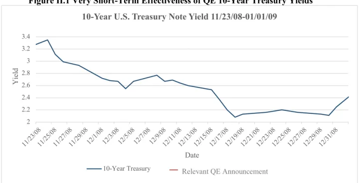
In this paper, we will assess the effects of quantitative easing over three time-periods on medium- and longer-term yields and the prices of financial assets within the U.S. Financial Markets. We will illustrate this via a time series analysis that will consider each relevant quantitative easing announcement10 _{from the FOMC during the Great Recession. Previous} literaturehas largely considered the immediate and short-term effects of signaling and the portfolio balance effect from the FOMC regarding LSAPs. Figure II.1 illustrates how this very short-term effect follows theory. A general consensus exists amongst the literature that, in the short-run, the FOMC’s QE policy lowered interest rates on longer-term securities by approximately 100bps. However, we agree with Greenwall (2018) that this overstates the true effect – especially over an extended period of time.

The short-run analysis from previous literature overlooks what we see to be a critical consideration in assessing the effectiveness of FOMC policy – its longevity. In order to form a comprehensive picture of the effectiveness of quantitative easing, a consideration of the long-run sustainability of the effect over a larger time period is necessary. In the longer term, additional

exogenous market factors likely alter the ability of QE policies to persist (see Figure II.2, Table II). In fact, the initial downward shift in the yield curve is often reversed or begins to reverse within

Figure II.1 Very Short-Term Effectiveness of QE 10-Year Treasury Yields

Data Source: FRED Federal Reserve Bank of St. Louis

Figure II.2 Longer-Term Effectiveness of QE on 10-Year Treasury Yields

Data Source: FRED Federal Reserve Bank of St. Louis 2 2.2 2.4 2.6 2.8 3 3.2 3.4 11/23 /08 11/25 /08 11/27 /08 11/29 /08 12/1/0812/3/0812/5/0812/7/0812/9/08_12/11 /08 12/13 /08 12/15 /08 12/17 /08 12/19 /08 12/21 /08 12/23 /08 12/25 /08 12/27 /08 12/29 /08 12/31 /08 Yi el d Date

10-Year U.S. Treasury Note Yield 11/23/08-01/01/09

10-Year Treasury 1 1.5 2 2.5 3 3.5 4 4.5 1/1/08 7/1/08 1/1/09 7/1/09 1/1/10 7/1/10 1/1/11 7/1/11 1/1/12 7/1/12 1/1/13 7/1/13 Yi ed Date

10-Year U.S. Treasury Note Yield 2008-2013

10-Year Treasury RelevantQEEventsAnnoucements

–

Figure III: Movement of Yield Curves Around Relative QE Announcements

Data Source: U.S. Department of the Treasury Table I: 1 Day Changes in Yields and Prices

Date 2-Year Treasury 10-Year Treasury 10-2 Treasury Spread BoAML BBB

Index S&P 500 VIX

11/25/08 -0.06 -0.12 -0.06 -0.05 $30.29 -5.98 12/1/08 0.00 -0.04 -0.04 0.06 $32.60 -5.53 3/18/09 0.05 0.10 0.05 0.07 -$10.31 3.62 11/3/10 -0.01 -0.14 -0.13 -0.11 $23.10 -1.04 9/21/11 -0.01 -0.16 -0.15 0.04 -$37.20 4.03 6/20/12 0.00 -0.02 -0.02 -0.03 -$30.18 2.84 9/13/12 0.03 0.13 0.10 0.00 $5.78 0.46 12/12/12 0.02 0.02 0.00 0.01 -$9.03 0.61 12/18/13 0.03 0.05 0.02 0.02 -$1.05 0.35

Table II: 1 Week Changes in Yields and Prices

Date Treasury 2-Year Treasury 10-Year 10-2 Treasury Spread BoAML BBB Index S&P 500 VIX

11/25/08 -0.25 -0.91 -0.66 -0.44 $10.76 -16.69 12/1/08 -0.15 -0.61 -0.46 -0.44 $74.43 -26.88 3/18/09 0.09 0.35 0.26 -0.29 $70.95 -4.27 11/3/10 0.15 0.36 0.21 0.35 $26.75 -1.55 9/21/11 0.07 0.32 0.25 0.28 $48.63 -2.54 6/20/12 -0.10 -0.11 -0.01 -0.28 $20.82 -1.79 9/13/12 0.03 -0.06 -0.09 -0.26 -$31.40 2.09 12/12/12 0.01 0.17 0.16 -0.06 $43.57 -2.59 0 0.5 1 1.5 2 2.5 3 3.5 4 4.5 1 Mo 3 Mo 6 Mo 1 Yr 2 Yr 3 Yr 5 Yr 7 Yr 10 Yr 20 Yr 30 Yr Yi el d to M at ur ity Time to Maturity

Yield Curves Pre & Post 11/3/2010 QE Announcement

a month of a QE Announcement (see Figure III)11_{. Thus, our objective is to investigate not just} whether or not LSAPs are effective but also as to whether or not a non-conventional monetary policy of this sort is sustainable over time.

II. Background II.1 Previous Literature

In 2004, then Federal Reserve Governors Ben S. Bernanke and Vincent R. Reinhart, and macroeconomist Brian P. Sack authored a paper entitled, “Monetary Policy Alternatives at the Zero Bound: An Empirical Assessment”. This paper addressed the policy options available to a central bank when nominal interest rates reach zero – or the “Zero-Lower Bound”. The zero-lower bound is the effective end of conventional monetary policy as the central bank can no longer utilize short-term interest rate changes to meet their monetary policy goals12_{. To this end, Bernanke} (2004) raised the question of whether or not unconventional monetary policies – specifically, LSAPs – would be effective in a modern, industrialized economy. While, at the time the paper was written, there was little likelihood of arriving at the zero-lower bound (with the exception of Japan), just four short years later, the authors’ work would be put to test in the open market.

While Bernanke, Reinhart, and Sack’s analyses are theoretically sound, their 2004 conclusions could not be tested until after the FOMC employed a non-conventional monetary policy during the Great Recession. Joseph Gagnon, Matthew Raskin, Julie Remache, and Brian Sack offer an empirical analysis of the FOMC’s LSAPs in their 2011 paper, “The Financial Market

11 _{See Appendix Figure III for the yield curves around each of the relevant QE Announcements.} 12 _{This holds true under the assumption that cash – being a perfectly liquid and risk-free asset –} offers a nominal return of 0%. Thus, if interest rates set by the FOMC were to turn negative and fall below the ZLB, investors would hold only cash and the negative interest rate policy would be moot.

Effects of the Federal Reserve’s Large-Scale Asset Purchases”. The authors provide extensive analysis on the short-run effects of QE. They conclude that the FOMC was largely successful in their objective13_.

Gagnon (2011) explains that the primary channel through which QE effected the financial markets to be the “portfolio balance” effect. Gagnon describes the portfolio balance effect’s mechanism as follows:

By purchasing a particular asset, a central bank reduces the amount of the security that the private sector holds, displacing some investors and reducing the holdings of others, while simultaneously increasing the amount of short-term, risk-free bank reserves held by the private sector. In order for investors to be willing to make those adjustments, the expected return on the purchased security has to fall. Put differently, the purchases bid up the price of the asset and hence lower its yield. (Gagnon, 6)

Gagnon explains that not only would this mechanism result in the yields of the securities being purchased by the central bank to fall, the effect would roll over into other similar securities via the substitution of similar financial assets. The intuition behind this comes from an investor’s tendency to purchase assets they see as a substitute for a given level of risk and liquidity when the expected return on the original asset falls14 _{(Gagnon, 8). Thus, the FOMC should be able to effectively} narrow the yields of various other debt instruments and change prices within the equity markets.

13 _{Gagnon says that in “reducing the net supply of assets with long duration, the Federal Reserve’s} LSAP programs appear to have succeeded in reducing the term premium…The overall size of the reduction in the ten-year term premium appears to be somewhere between 30 and 100 basis points, with most estimates in the lower and middle thirds of this range.” (Gagnon, 38).

14 _{We illustrate this effect via an analysis of the yields on the Bank of America Merrill-Lynch BBB} Corporate Bond Index.

Most recently, David Greenwall, James D. Hamilton, Ethan S. Harris, and Kenneth D. West’s 2018 paper, “A Skeptical View of the Impact of the Fed’s Balance Sheet”, argues that previous literature tends to overstate and actual effectiveness of the FOMC’s LSAP policy and that the use of conventional monetary policy to alter the FFR is more reliable. Greenwall’s analysis focuses on the effect of LSAPs on 10-year Treasuries using an event study approach. Greenwall observes that while yields do move as would be expected in the very short run, the effect is not lasting. To this, the authors explain that “possible explanations include initial market overreaction and the failure of the Fed to meet market expectations” and “that Treasury actions offset Fed purchases” (Greenwall, 2018). This gives way to their overall conclusion that LSAPs effect yields only modestly – and certainly less than what previous literature claims.

II.2 The Longer-Term

The mechanism described by Bernanke (2004) and Gagnon (2011) seems to be very effective in the immediate to short-run (as is illustrated in Figure I.1 and Table I). The supply of debt securities available to investors on the open market does shrink upon the Federal Reserve purchase of said securities. However, this theory requires ceteris paribus of a number of exogenous variables which, in a developed economy, will not hold. Thus, what is likely to occur in reality are successful results of non-conventional monetary policy in the short-run that do not hold in the long-run.

The rationale as to why the effects of QE appear to be short-lived are twofold. First, the portfolio balance effect itself might be generally short-lived. This would occur after the initial adjustment in price from the Fed’s manipulation of supply, investors may find suitable substitute investment opportunities given their level of risk tolerance and required return. For example, when the yield on a fixed-income security decreases due to a market manipulation (e.g. a decrease in the

supply due to the FOMC’s LSAPs) without a change in risk or variance, the expected return on the security is likely to fall below the required return. When this occurs, a portfolio manager or investor will underweight that security in favor of some other substitute security that will provide their required return. This substitution of assets in this scenario would result in a lower demand in the open market for the securities the FOMC had been purchasing thereby causing a decrease in price and, therefore, an increase in yields over an extended period of time.

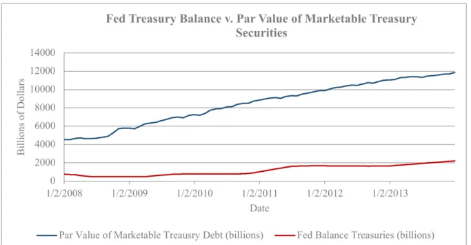
The second rationale we consider is the effect of the U.S. Treasury Department’s own agenda – specifically the Treasury’s issuance of new debt. The Bernanke (2004) model does not take changes in the overall level of marketable securities via new issues into consideration. While this may have been satisfactory in the purely theoretical analysis of pre-recession papers (e.g. Bernanke 2004), it is well known that such an assumption (constant level of supply of marketable treasury, agency debt, and MBS securities, etc.) is not characteristic of the financial markets. Especially given that throughout the course of the Great Recession, the Congress passed multiple pieces of stimulus fiscal policy. Policy actions that were at least partially funded by the issuance of new U.S. Government Debt from the U.S. Treasury. Thus, it is a known fact that the par value of marketable U.S. Treasury Securities was fluid and increasing throughout the same time period when the Fed was employing its LSAPs (see Figure IV).

Thus, move outside of a theoretical environment and the mechanism described by Bernanke (2004) and again by Gagnon (2011) begins to deteriorate. The U.S. Department of the Treasury underwrites U.S. Treasury Debt of various maturities through the course of each month. This would have little if any effect when looking at the portfolio balance effect on an intraday to one-day time-frame. However, increase the time parameter and the par-value of marketable U.S. Treasury Debt will have increased – by a potentially significant amount. This would seem to

suggest that, in the longer-term, the narrowed yields would begin to widen again as the price of debt securities is driven down by an increase in supply via new debt issues.

The discussion from Greenwall (2018) explains that throughout this time-frame, the “Treasury’s own objectives for its maturity risk15 _{led it to increase the average maturity of} outstanding Treasury debt over the 2009-2017 period, offsetting and even reversing the efforts by the Fed” (Greenwall, 2018). The resulting implications of this continuously increasing level of supply would be much the opposite of the FOMC’s desired policy effect. Our findings indicate that these implications are correct – the daily change in the par value of marketable U.S. Treasury Securities had a positive effect on the 10-year Treasury yield at a statistically significant level. Figure IV: Difference in Fed Treasury Purchases and New Issues

Data Source: Federal Reserve Bank ofNew York & the U.S. Department of the Treasury

15 _{The Maturity Risk Premium (MRP) is an added premium to a security’s yield in order to} compensate for the expected interest rate risk.

0 2000 4000 6000 8000 10000 12000 14000 1/2/2008 1/2/2009 1/2/2010 1/2/2011 1/2/2012 1/2/2013 Bi lli on s of Do lla rs Date

Fed Treasury Balance v. Par Value of Marketable Treasury Securities

This would suggest that the QE policies pursued by the FOMC did not have the sustainability of a policy that generates long-term policy results. Rather, it appears that QE is similar to ibuprofen – it reverses the symptoms for the time being, but if you wish the desired effect to continue, you must take additional doses. This is precisely what the FOMC did. After QE1 was announced on November 25, 2008, there were six additional statements16 _announcing additional LSAPs by the Fed after FOMC meetings.

That is not to say that the policy actions of the Federal Reserve had no expansionary effect on the struggling U.S. Economy. While we believe the longer-term effectiveness of the FOMC’s QE Policy was moot due to other exogenous factors, we believe that there was immediate-/short-term impact that followed the theory developed by Bernanke (2004). Furthermore, we believe this to be a statistically significant short-term effect as has been concluded by the previous literature. III. Data

The data used in this paper are readily available from the Federal Reserve Bank of St. Louis’s FRED, the Federal Reserve Bank of New York, the U.S. Department of the Treasury, and Bloomberg. The majority of the data used in our analysis was reported on a daily basis. There were, however, some key variables which were reported on different time scales. In order to use these important pieces of data in our analysis, we had to establish a method of estimating the daily value of these data. While an imperfect measure to be sure, we used a linear approximation to do this. To achieve this, the change in value from one observation to the next was calculated. This was then divided by the number of days in which the U.S. Financial Markets were open between

16 _{These statements were issued on March 19, 2009 (QE1), November 3, 2010 (QE2), September} 21, 2011 (OT), June 20, 2012 (OT), September 13, 2012 (QE3), and December 12, 2012 (QE3). Note that in most cases, there was a second purchase announcement for each program within 1 fiscal quarter of the first announcement. The exception to this was the Maturity Extension program.

the observations. Finally, in order to find the value at any given day, the estimated daily change17 was added to the initial value. This process was used for the U6 Rate of Unemployment, Personal Consumption Expenditure (PCE), Seasonally Adjusted Real GDP, and Par Value of Marketable Treasury Securities18 _data.

Given the importance of changes over time in our analysis, additional time-lagged and leading variables were generated. A lagged variable for each data was created for the previous week, and previous day; a leading variable was generated for next day, one-week, and one-month. This allowed us to control for previous prices in our model as well as to analyze whether or not the Fed’s policy changes were pre-priced into the market. The data were lagged by the number of days the financial markets were open (i.e. a one-week lag would be lagged by 5 days, etc.)

IV. Methodology & Discusssion IV.1 Econometric Models

We begin our econometric analysis by considering the immediate- and short-term effects of relevant QE announcements on five classes of financial assets – U.S. Treasury Securities (both Two-Year and Ten-Year Treasury Notes), Agency Mortgage Backed Securities, Corporate Debt Securities, and Equities.

Our econometric analysis was performed using three regressions for each security’s yield or price being tested. The first regression was conducted as a baseline which estimated the dependent variable (the yield or price of the security in question) as a function of the quantitative easing announcement dummy and the dependent variable’s price from the previous week.

17 _{It is important to note that this is not a fully accurate representation of what the actual daily} values of these variables would be. Rather, it provided us with an approximation to aid in our analysis.

18 _{The Par Value of Marketable Treasury Securities is used as the level of supply of Treasury} Securities available for purchase in the open market.

(1) y= β₁RelevantQEAnnouncement + β₂y_PriorWeek + ε

i

y = security yield/price

yPriorWeek= asset yield/price from one-week (5 business days) prior

Next, macroeconomic and market control variables were attend to control for other happenings in the financial markets and eliminate omitted variable bias in the model. The control variables used in this model were the U6 measure of unemployment, the Core Personal Consumption Expenditures Index, Seasonally Adjusted Real GDP, the value of the S&P 500 index, and the value of the CBOE VIX Volatility Index.

(2) y = β₁RelevantQEAnnouncement + β₂y_PriorWeek + β₃U6 + β₄CorePCE

+ β₅RealGDP + β₆S&P500 + β₇VIXIndex + εi

yPriorWeek = asset price/yield from one-week (5 business days) prior

U6 = U6 measure of unemployment

CorePCE = PCE prices excluding food and energy prices RealGDP = Seasonally Adjusted Real GDP

S&P500 = Price of the S&P 500 at market close

VIXIndex = Volatility as measured by the CBOE VIX Index at market close Finally, the daily change in par value of marketable U.S. Treasuries was added to the model in order to quantify the effect of changes in the supply of Treasury Securities available on the open market from the U.S. Treasury’s issuance of new Treasury debt in the financial markets.

(3) y = β₁RelevantQEAnnouncement + β₂y_PriorWeek + β₃U6 + β₄CorePCE

+ β₅RealGDP + β₆S&P500 + β₇VIXIndex + β₈ PVTresChange_PriorWeek + εi1920

yPriorWeek = asset price/yield from one-week (5 business days) prior

19 _{This regression was run in two ways: (3.1) included the Daily Change in Present Value of} Marketable Treasury Securities from the prior day and from the prior week, (3.2) included only the value from the prior week. Both the prior day and prior week present value variables illustrate the same overall effect (both show upward pressure on Treasury yields) however, the prior week variable provides a stronger effect and thus is the measure included in the main analysis. See Appendix Table II for both regressions.

20 _{The models for the one-week and one-month time-periods also include the yield/price at t = 0} in the regression model. See Appendix Equations I-II for the full regression model for these time-periods.

U6 = U6 measure of unemployment

CorePCE = PCE prices excluding food and energy prices RealGDP = Seasonally Adjusted Real GDP

S&P500 = Price of the S&P 500 at market close

VIXIndex = Volatility as measured by the CBOE VIX Index at market close PVTresChange = Daily growth rate of the par value of market treasury securities

Given that these models include the previous week’s price as an explanatory variable, we expected the r-squared values to be quite high. As such, both the r-squared values and the root mean squared error values are considered in determining the strength of each model.

Using these models, regressions for three different time frames were conducted in order to identify (1) the immediate- to short-term effect of QE announcements, from market close the prior day to market close the day of an announcement (2) the longer-term effects after one week, and (3) the longer-term effects after one month has passed. In order to better analyze the effect on the markets as a whole, regressions were run on a range of financial securities. While these securities were primarily fixed income instruments – as both the immediate effect of LSAPs and the portfolio balance effect would most easily be seen here – the price of the Standard & Poors 500 Index was also included21_.

IV.2 10-Year Treasury Note

The 10-Year Treasury Note was of particular interest as it should best reflect the effect of QE given that LSAPs target longer-term interest rates. As is consistent with previous literature, we find that there is a statistically significant immediate negative effect on yields when the FOMC makes a QE announcement. In the immediate-term, this is significant at the one-percent level for each of the

21 _{The securities used were the: 10-Year Treasury Note, 2-Year Treasury Note, 10-Year – 2-Year} Treasury Spread, Bank of America Merrill Lynch BBB Bond Index, Bloomberg MBS Index, and the S&P 500

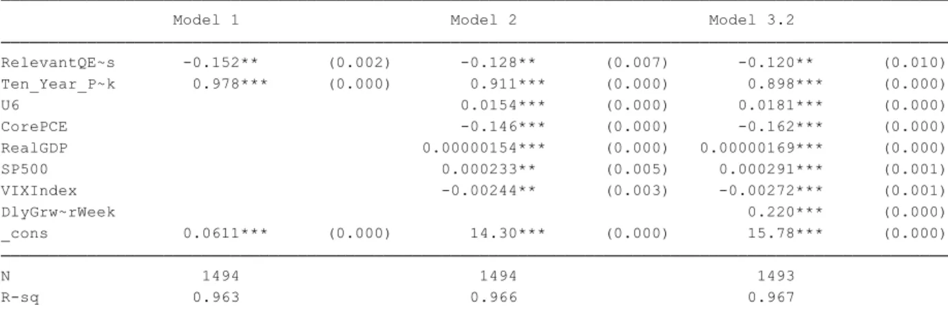
three regression models. In Model (3) – the model with the highest explanatory power22 _{– a QE} announcement would result in a decrease of 12bps (see Figure IV). That is to say, in the immediate-term, the FOMC was successful in their usage of LSAPs to lower longer-term interest rates.

Each variable in this model is significant at the one-percent level albeit the effect of some of the controls (e.g. the S&P500 Index, the VIX Index, and Real GDP have less than a 1bps effect on the 10-Year Treasury Yield). As we hypothesized, increases in the par value of marketable treasury securities does have a positive effect on yields – in this case pushing them up by approximately 22bps for every one-percent increase in the supply of Treasuries. However, this counter-effect would not be seen in the immediate term as the par value of new treasury issues would not be that large in one day. Our results from the second time-frame – one week later – provides results that are somewhat less straight forward. In this time-frame, variables were lagged by one business week (i.e. 5 days) in order to isolate the effect of a QE Announcement after the market has had a full week to fully price the policy change into prices and therefore yields. The explanatory power of the three regressions remained just about the same based on the R-Square and Root MSE values23_{. However, after one week, Model (3) estimates that when there was a QE} announcement one business week prior yields on the 10-Year Treasury would increase by 2.8bps (see Figure IV). This statistic is not, however, statistically significant. The reason behind this change in significance and value is not entirely clear though it may be due to a decrease in market demand for the asset thereby causing the price to fall and yields to rise.

22 _{Model 3 for the immediate term has an Adjusted R-Squared of 0.9667 and a Root MSE of} 0.13898 compared to Model 2’s Adjusted R-Squared of 0.9663 and Root MSE of 0.13986 and Model 1’s Adjusted R-Squared of 0.9633 and Root MSE of 0.14588.

23 _{See Appendix Table III for R-Squared, Adjusted R-Squared, and Root MSE values for each of} the three regressions in each of the three time-periods.

The time-period of greatest interest to us was the longer-term (i.e. one-month post announcement24_{) time-frame. In this time-frame we believe the market will have had sufficient} time to synthesize the initial new information from QE announcements in addition to market responses and changes in the supply of Treasury Securities. Of key interest in this set of regressions are the estimated beta values of ß1 and ß8. ß1 estimates that a QE announcement one month prior causes the 10-Year Treasury Yield to be depressed by 13.33bps and is statistically significant at the ten-percent level (see Figure IV). This is consistent with our hypothesis that, over time, the FOMC’s QE announcements had a lesser market moving effect. While there was still likely downward pressure on long-term interest rates, this value is less statistically significant than it was when considering the effect in the immediate term. Given that the supply of Treasury securities available on the open market were controlled for in our analysis, the loss of significance at both the one-week and one-month time periods is evidence that the portfolio balance effect had only a short-term negative impact on yields.

Furthermore, the hypothesis that the growth in new Treasury securities (as measured by the par value of new U.S. Treasury Issues) offset the downward effect of LSAPs on yields proved to be correct. Our model estimated a beta of approximately .58 (58bps) for the effect of the daily growth in the par value of new U.S. Treasury issues (see Figure IV). This estimate is significant at the .1% significance level. Thus, it is evident that the growth in the supply of Treasuries caused prices to fall by an amount greater than the increase in price from the FOMC’s LSAPs thereby

24 _{Admittedly, the length of time that has passed does create more variability in our model – both} the Adjusted R-Squared and the Root MSE values show that the explanatory power of the model decreased. That decrease, however, was only a slight decrease and we are still confident in the results of the model.

Figure V: 10-Year Treasury Regression Results * p<0.05, ** p<0.01, *** p<0.001 p-values in parentheses R-sq 0.963 0.966 0.967 N 1494 1494 1493 _cons 0.0611*** (0.000) 14.30*** (0.000) 15.78*** (0.000) DlyGrw~rWeek 0.220*** (0.000) VIXIndex -0.00244** (0.003) -0.00272*** (0.001) SP500 0.000233** (0.005) 0.000291*** (0.001) RealGDP 0.00000154*** (0.000) 0.00000169*** (0.000) CorePCE -0.146*** (0.000) -0.162*** (0.000) U6 0.0154*** (0.000) 0.0181*** (0.000) Ten_Year_P~k 0.978*** (0.000) 0.911*** (0.000) 0.898*** (0.000) RelevantQE~s -0.152** (0.002) -0.128** (0.007) -0.120** (0.010) Model 1 Model 2 Model 3.2 10-Year Treasury 1-Day

* p<0.05, ** p<0.01, *** p<0.001 p-values in parentheses R-sq 0.963 0.967 0.967 N 1489 1489 1489 _cons 0.0537*** (0.000) 15.27*** (0.000) 16.56*** (0.000) DlyGrwthT~ly 0.218*** (0.000) VIX_1Week -0.00308*** (0.000) -0.00335*** (0.000) SP500_1Week 0.000198* (0.020) 0.000253** (0.003) RealGDP_1W~k 0.00000172*** (0.000) 0.00000184*** (0.000) CorePCE_1W~k -0.155*** (0.000) -0.169*** (0.000) U6_1Week 0.0136** (0.002) 0.0163*** (0.000) Ten_Year_P~k 0.0831** (0.001) 0.0971*** (0.000) 0.0947*** (0.000) Ten_Year 0.897*** (0.000) 0.819*** (0.000) 0.810*** (0.000) RelevantQE~s 0.0139 (0.777) 0.0253 (0.591) 0.0282 (0.546) Model 1 Model 2 Model 3.2 10-Year Treasury 1-Week

* p<0.05, ** p<0.01, *** p<0.001 p-values in parentheses R-sq 0.897 0.918 0.921 N 1479 1479 1479 _cons 0.166*** (0.000) 35.80*** (0.000) 37.82*** (0.000) DlyGrw~1Week 0.583*** (0.000) VIX_1Month -0.00238 (0.072) -0.00370** (0.005) SP500_1Month 0.000919*** (0.000) 0.00102*** (0.000) RealGDP_1M~h 0.00000358*** (0.000) 0.00000373*** (0.000) CorePCE_1M~h -0.370*** (0.000) -0.392*** (0.000) U6_1Month 0.0507*** (0.000) 0.0548*** (0.000) Ten_Year_1~k 1.005*** (0.000) 0.834*** (0.000) 0.814*** (0.000) Ten_Year -0.0654 (0.130) -0.0829* (0.036) -0.0880* (0.023) RelevantQE~s -0.114 (0.189) -0.143 (0.066) -0.133 (0.082) Model 1 Model 2 Model 3.2 10-Year Treasury 1-Month

causing yields to rise more than QE caused them to fall. The effectiveness of the FOMC’s QE policy is therefore curtailed by exogenous market factors.

IV.3 2-Year Treasury Securities

The theory surrounding QE holds that this nonconventional monetary policy should have little effect on the yields of shorter-term securities given that the LSAP policy purchases longer-term securities from the open market. However, we are interested in the rollover effect that QE had on the yields of shorter-term securities. Given that this type of monetary policy would result in a flattening of the yield curve due to lower yields on longer-maturity instruments, relatively little should happen to the yield on the 2-Year Treasury Note in response to a QE Announcement. This is the case since the FOMC had already lowered short-term rates to the ZLB which would have had a more significant effect on the 2-Year yield than the FOMC’s purchase of Treasuries with longer maturities (see Appendix Table IV for a comparison of the 10-Year and 2-Year Treasuries).

Following this theory, we find that none of the regressions and time-periods support a statistically significant effect of a relevant QE announcement on the 2-Year Treasury Note. At best, a relevant QE announcement is only significant at the 30% level on Regression 3.2 during the 1-Week time-period (see Figure VI). Additionally, we find that new issues of Treasury Securities also did not have a statistically significant effect in the yield of 2-Year Treasuries. Therefore, we conclude that LSAPs do not have a powerful impact on the yields of 2-Year Treasury Securities.

* p<0.05, ** p<0.01, *** p<0.001 p-values in parentheses R-sq 0.974 0.977 0.977 N 1494 1494 1493 _cons 0.0142*** (0.001) -0.167 (0.919) -0.0270 (0.987) DlyGrw~rWeek 0.0225 (0.522) VIXIndex -0.00301*** (0.000) -0.00308*** (0.000) SP500 0.0000730 (0.137) 0.0000745 (0.130) RealGDP -0.000000604* (0.023) -0.000000588* (0.027) CorePCE 0.00644 (0.697) 0.00504 (0.761) U6 -0.0162*** (0.000) -0.0163*** (0.000) Two_Year_P~k 0.972*** (0.000) 0.852*** (0.000) 0.851*** (0.000) RelevantQE~s -0.0476 (0.171) -0.0322 (0.332) -0.0314 (0.344) Model 1 Model 2 Model 3.2 2-Year Treasury 1-Day

* p<0.05, ** p<0.01, *** p<0.001 p-values in parentheses R-sq 0.974 0.977 0.977 N 1489 1489 1489 _cons 0.0117** (0.005) 0.650 (0.693) 0.654 (0.692) DlyGrwthT~ly 0.00179 (0.959) VIX_1Week -0.00343*** (0.000) -0.00343*** (0.000) SP500_1Week 0.0000439 (0.370) 0.0000441 (0.370) RealGDP_1W~k -0.000000426 (0.110) -0.000000426 (0.110) CorePCE_1W~k -0.00186 (0.910) -0.00189 (0.909) U6_1Week -0.0150*** (0.000) -0.0150*** (0.000) Two_Year_P~k 0.134*** (0.000) 0.126*** (0.000) 0.126*** (0.000) Two_Year 0.840*** (0.000) 0.740*** (0.000) 0.740*** (0.000) RelevantQE~s 0.0216 (0.530) 0.0354 (0.281) 0.0355 (0.281) Model 1 Model 2 Model 3.2 2-Year Treasury 1-Week

* p<0.05, ** p<0.01, *** p<0.001 p-values in parentheses R-sq 0.934 0.950 0.950 N 1479 1479 1479 _cons 0.0282*** (0.000) 1.692 (0.484) 1.676 (0.488) DlyGrw~1Week -0.0642 (0.216) VIX_1Month -0.00725*** (0.000) -0.00704*** (0.000) SP500_1Month 0.000143* (0.046) 0.000139 (0.053) RealGDP_1M~h -0.000000988* (0.011) -0.000000974* (0.013) CorePCE_1M~h -0.00677 (0.780) -0.00674 (0.781) U6_1Month -0.0348*** (0.000) -0.0341*** (0.000) Two_Year_1~k 0.866*** (0.000) 0.646*** (0.000) 0.647*** (0.000) Two_Year 0.0709 (0.076) 0.0467 (0.197) 0.0508 (0.162) RelevantQE~s -0.0288 (0.617) -0.0398 (0.428) -0.0412 (0.413) Model 1 Model 2 Model 3 2-Year Treasury 1-Month

IV.4 Mortgage Backed Securities (MBS) – Bloomberg 30-Year Ginnie Mae Mortgage Rate

The other asset class the FOMC’s LSAPs had a direct impact on was the Mortgage Backed Security. The Fed had begun to acquire and hold MBSs on their balance sheet via LSAPs from the very onset of their QE program, even before they had begun purchasing U.S. Treasury securities25_. It should then follow that relevant QE announcements result in a statistically significant decrease in yields resulting from the Fed driving up the price of MBS decreasing the supply of Agency MBS on the open market. Our analysis proves this to be correct in the short-run though somewhat ambiguous when considering the effects over time.

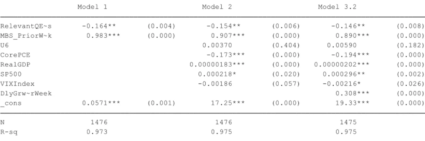
The models show that the yield on the 30-Year Ginnie Mae Mortgage Backed Security (MBS) follows the same initial trend as the yield of the 10-Year Treasury. Model (3) again has the greatest explanatory power of the three regression models used. At the one-day time-frame, a relative quantitative easing announcement has an estimated 14.6bps decrease on the yield of the MBS at the one-percent significance level (see Figure V). Unlike the 10-Year Treasury Yield, however, the macro- and market effects controlled for in the model have less influence on the MBS yield. While all but the U6 rate of unemployment are statistically significant at the five-percent level, only relative QE announcements, the previous week’s MBS yield, Core PCE, and the daily growth in new Treasury issues have an impact of at least one basis point up or down. Additionally, slightly more of the variation in the yield of the MBS is explained at the initial time-period than the 10-Year Treasury26_{. These results are consistent with both previous literature and our}

25 _{Purchases of MBS were conducted under QE1, QE2, and QE3. QE1 allowed for LSAPs of} Agency MBS to total $1.25 trillion ($500 billion from phase one and $750 billion from phase two) (Rosengren, 2015).

26 _{The R-Squared from Model (3) at the initial time-period is 0.975 compared to 0.967 for the} 10-Year Treasury

Figure V: 30-Year Mortgage Backed Security Regression Results * p<0.05, ** p<0.01, *** p<0.001 p-values in parentheses R-sq 0.973 0.975 0.975 N 1476 1476 1475 _cons 0.0571*** (0.001) 17.25*** (0.000) 19.33*** (0.000) DlyGrw~rWeek 0.308*** (0.000) VIXIndex -0.00186 (0.057) -0.00216* (0.026) SP500 0.000218* (0.020) 0.000296** (0.002) RealGDP 0.00000183*** (0.000) 0.00000202*** (0.000) CorePCE -0.173*** (0.000) -0.194*** (0.000) U6 0.00370 (0.404) 0.00590 (0.182) MBS_PriorW~k 0.983*** (0.000) 0.907*** (0.000) 0.890*** (0.000) RelevantQE~s -0.164** (0.004) -0.154** (0.006) -0.146** (0.008) Model 1 Model 2 Model 3.2 30-Year MBS 1-Day * p<0.05, ** p<0.01, *** p<0.001 p-values in parentheses R-sq 0.970 0.976 0.976 N 1469 1465 1465 _cons 0.0436* (0.013) 19.13*** (0.000) 21.19*** (0.000) DlyGrwthT~ly 0.327*** (0.000) VIX_1Week -0.00384*** (0.000) -0.00423*** (0.000) SP500_1Week 0.0000845 (0.370) 0.000158 (0.094) RealGDP_1W~k 0.00000226*** (0.000) 0.00000245*** (0.000) CorePCE_1W~k -0.190*** (0.000) -0.212*** (0.000) U6_1Week -0.00131 (0.766) 0.000780 (0.858) MBS_PriorW~k 0.197*** (0.000) 0.221*** (0.000) 0.225*** (0.000) MBS 0.789*** (0.000) 0.705*** (0.000) 0.684*** (0.000) RelevantQE~s 0.0233 (0.701) 0.0260 (0.633) 0.0278 (0.605) Model 1 Model 2 Model 3.2 30-Year MBS 1-Week * p<0.05, ** p<0.01, *** p<0.001 p-values in parentheses R-sq 0.929 0.946 0.947 N 1453 1449 1449 _cons 0.141*** (0.000) 46.57*** (0.000) 44.34*** (0.000) SP500_1Month 0.000676*** (0.000) DlyGrw~1Week 0.302*** (0.001) VIX_1Month -0.00948*** (0.000) -0.00429** (0.005) RealGDP_1M~h 0.00000568*** (0.000) 0.00000469*** (0.000) CorePCE_1M~h -0.459*** (0.000) -0.446*** (0.000) U6_1Month -0.0148*** (0.000) 0.0112 (0.090) MBS_1Week 0.961*** (0.000) 0.797*** (0.000) 0.759*** (0.000) MBS -0.00503 (0.904) 0.0240 (0.524) 0.00744 (0.843) RelevantQE~s -0.00752 (0.939) -0.0565 (0.511) -0.0457 (0.592) Model 1 Model 2 Model 3 30-Year MBS 1-Month

hypothesis. The immediate effects of QE do lower longer-term yields on securities purchased by the FOMC.

Just as occurred for the 10-Year Treasury Yield, our analysis shows that after one-week, Model (3) estimates that when there was a QE announcement one business week prior yields on the 10-Year Treasury would increase – for the MBS by 2.78bps. However, for the MBS, this is 6% less significant; the increase is significant only at the approximately 61% level. This is consistent with our hypothesis that the effects of QE start to dull with the passing of time and the changing of exogenous market forces.

In time period 3, we find that relevant QE announcements resulted in a 4.6bps decrease in yield at an insignificant level (see Figure V). This is further evidence that the portfolio balance effect, which drove the initial decrease in yields immediately following a relevant QE announcement, is a short-term effect; in the longer-term, investors and portfolio managers have sufficient time to substitute securities in their portfolio to meet their required return. Additionally, our model shows that the yield of the MBS during this time-period was driven by the growth in marketable Treasury securities far more than by the FOMC’s QE policy. For every 1% increase in the par value of marketable treasury securities, the yield on the 30-Year MBS is estimated to increase by 30.2bps. Furthermore, this is statistically significant at the 0.1% significance level. This result shows that as the time-period being considered extends in duration, the effectiveness of the FOMC’s LSAPs begins to dwindle. Likewise, this result confirms our belief that the continuous increases in the supply of treasuries would have an effect not just on treasuries, but also on the yields of other securities in the market27_.

27 _{One explanation for the rollover into MBSs is the substitution effect. As the price of Security B} (call it the 10-Year Treasury) decreases due to an increase in supply, demand for Security A (let’s

IV.5 Other Securities

Theory holds that the FOMC’s QE purchases should result in a rollover effect on the yields and prices of other related financial securities due to the portfolio balance effect. We will address two such securities – BBB corporate bonds as measured by the Bank of America Merrill-Lynch BBB Bond Index (BAML BBB) and large cap equities as measured by the S&P 500 Index. In considering the initial effects of QE on the BAML BBB, we find a lower and far less significant effect of QE on the security’s yield. Our model estimates that a relevant QE announcement would result in a same day decrease of just 2.87bps at approximately the 50% significant level – a far cry from significance. This is almost 10bps less than the effect relevant QE announcements had on the Figure VI: Daily Percent Change in BAML BBB & 10-Year Treasury Yield

10-Year Treasury note and approximately 12bps less than the effect on MBS (see Figures VI & VII). We do observe a greater effect of changes in the VIX Index on the BAML BBB than we did

say the 30-Year MBS) falls as investors move their money to the relatively less expensive Security B thereby reducing the price of Security B and resulting in an increase in yield on Security B.

-20.00 -17.50 -15.00 -12.50 -10.00 -7.50 -5.00 -2.50 0.00 2.50 5.00 7.50 3/11/09 3/18/09 3/25/09 4/1/09 4/8/09 4/15/09 Da ily P er ce nt Ch an ge in Yi el d

Daily Rate of Change March 18, 2009 QE Announcement

on the 10-Year Treasury and the MBS – an increase in the volatility in of 1 results in an estimated increase in yield by 0.7bps.

The effect of relevant QE announcements on the BAML BBB yield solidifies over-time though the estimated change in yield is still less and far less significant than the effect on the 10-Year Treasury. This confirms the theory that the FOMC’s use of QE did roll over onto other securities though the extent is far less than one-to-one. Model (2) at time 3 (1-month later) estimates that a relevant QE announcement will result in a 12.4bps decrease in BBB Corporate Bond yields at the 15% significance level. Model (2), however, does not have the most explanatory power – as in all of the other regressions in our analysis, Model (3) explains the most variation28_{. This model} estimates that a relevant QE announcement will result in an approximately 7.4bps decrease in BAML BBB yield in time period 3. This change is significant at the 35% level – 15% more significant as the first time period though not as significant as Model (2) in the third time period. Thus, it is likely that the use of QE by the FOMC did have some roll-over effect onto corporate securities in the fixed-income market. However, as is shown above, the longer the time-frame considered, the more exogenous market factors make the effect less and less significant.

That being said, throughout the entirety of our analysis of the BAML BBB, market volatility as measured by the CBOE VIX has very significant and persistent effects. Based on regression model 3, during all three time periods considered, a one-point increase in volatility results in a 0.79-2.10bps increase in BBB yield with a 0.1% significance level. The result is the strongest during the third time period at a rate of 2.10bps per 1 point of volatility. This makes sense given that investors should require additional yield on somewhat riskier fixed-income securities (such as

28 _{BAML BBB Model 2 has an R-squared value of 0.983 and a Root MSE of 0.23374 while Model} 3 has an R-squared value of 0.985 and a Root MSE of 0.21933.

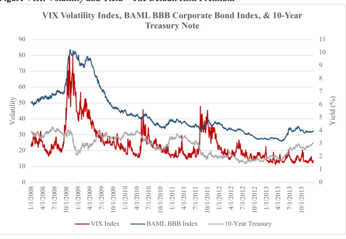
BBB corporates) when volatility in the market increases. Increased volatility in the financial markets can result in investors perceiving default to be a greater risk – especially for companies with lower credit ratings such as BBB. As a result, investors will demand more compensation for holding this perceived risk via a larger default risk premium on corporate debentures which are backed only by the general credit worthiness of the company. The same effect of volatility on yield is not observed on U.S. Treasury securities. This is likely due to the fact that Treasuries are backed by the full faith and credit of the United States Government. Thus, Treasuries are viewed as virtually risk-free assets and therefore do not pay a default risk premium. Hence, when volatility in the market increases, investors do not require more yield from Treasury securities as they do for other securities29 _{(see Figure VIII).}

Figure VIII: Volatility and Yield – The Default Risk Premium

29 _{Appendix Table V contains the correlations between the five asset classes and both the VIX} Index and Relevant QE Announcement variable to illustrate this further.

0 1 2 3 4 5 6 7 8 9 10 11 0 10 20 30 40 50 60 70 80 90 1/ 1/ 2008 4/ 1/ 2008 7/ 1/ 2008 10/ 1/ 200 8 1/ 1/ 2009 4/ 1/ 2009 7/ 1/ 2009 10/ 1/ 200 9 1/ 1/ 2010 4/ 1/ 2010 7/ 1/ 2010 10/ 1/ 201 0 1/ 1/ 2011 4/ 1/ 2011 7/ 1/ 2011 10/ 1/ 201 1 1/ 1/ 2012 4/ 1/ 2012 7/ 1/ 2012 10/ 1/ 201 2 1/ 1/ 2013 4/ 1/ 2013 7/ 1/ 2013 10/ 1/ 201 3 Yi el d (% ) Vo la til ity

VIX Volatility Index, BAML BBB Corporate Bond Index, & 10-Year Treasury Note

Figure VII: Bank of America Merrill-Lynch BBB Bond Index * p<0.05, ** p<0.01, *** p<0.001 p-values in parentheses R-sq 0.993 0.994 0.995 N 1494 1494 1493 _cons 0.00834 (0.490) 0.414 (0.865) 2.662 (0.253) DlyGrw~rWeek 0.560*** (0.000) VIXIndex 0.00956*** (0.000) 0.00791*** (0.000) SP500 0.000231** (0.001) 0.000211** (0.002) RealGDP -0.000000221 (0.551) 0.000000145 (0.682) CorePCE -0.00474 (0.844) -0.0272 (0.238) U6 -0.00848* (0.023) -0.00966** (0.007) BAMLBBB_Pr~k 0.997*** (0.000) 0.949*** (0.000) 0.948*** (0.000) RelevantQE~s -0.0220 (0.659) -0.0489 (0.276) -0.0287 (0.501) Model 1 Model 2 Model 3.2 BAML BBB 1-Day * p<0.05, ** p<0.01, *** p<0.001 p-values in parentheses R-sq 0.993 0.994 0.995 N 1489 1489 1489 _cons 0.0147 (0.215) 1.558 (0.527) 3.051 (0.194) DlyGrwthT~ly 0.566*** (0.000) VIX_1Week 0.00882*** (0.000) 0.00793*** (0.000) SP500_1Week 0.000193** (0.007) 0.000213** (0.002) RealGDP_1W~k -5.14e-08 (0.890) 0.000000191 (0.590) CorePCE_1W~k -0.0156 (0.522) -0.0311 (0.181) U6_1Week -0.00926* (0.013) -0.00997** (0.005) BAMLBBB_Pr~k -0.215*** (0.000) -0.0750** (0.003) 0.0119 (0.632) BAMLBBB 1.211*** (0.000) 1.023*** (0.000) 0.935*** (0.000) RelevantQE~s 0.0864 (0.076) 0.0583 (0.193) 0.0693 (0.105) Model 1 Model 2 Model 3.2 BAML BBB 1-Week * p<0.05, ** p<0.01, *** p<0.001 p-values in parentheses R-sq 0.973 0.983 0.985 N 1479 1479 1479 _cons 0.0696** (0.004) 13.65** (0.002) 14.00*** (0.001) DlyGrw~1Week 1.167*** (0.000) VIX_1Month 0.0240*** (0.000) 0.0210*** (0.000) SP500_1Month 0.000369** (0.004) 0.000425*** (0.000) RealGDP_1M~h 0.00000123 (0.065) 0.00000133* (0.033) CorePCE_1M~h -0.134** (0.002) -0.139*** (0.001) U6_1Month -0.0323*** (0.000) -0.0339*** (0.000) BAMLBBB_1W~k 1.680*** (0.000) 1.133*** (0.000) 0.972*** (0.000) BAMLBBB -0.696*** (0.000) -0.289*** (0.000) -0.124** (0.004) RelevantQE~s -0.235* (0.024) -0.124 (0.137) -0.0744 (0.339) Model 1 Model 2 Model 3 BAML BBB 1-Month

In addition to the roll-over effects in the corporate fixed-income market, we consider the effects in the equity market. While the effects of LSAPs in this sector of the financial markets will likely be more difficult to isolate, they are nevertheless important to consider in order to understand the overall effect of LSAPs in the U.S. Financial Markets. Since LSAPs have no direct effect on the S&P 500, Model 2 is the best model to show to what extent, if any, QE had on the equity market. While it was necessary to add all market and macroeconomic controls to the analysis of the S&P 500, adding the supply of Treasuries data was not. The par value of marketable treasuries proved to be of importance in our fixed-income analysis due to the direct or indirect influence the supply of Treasuries had on prices and yields. As no such influence existed in the equities market, we believe Model (2) to be the best model for analysis of the S&P 50030_.

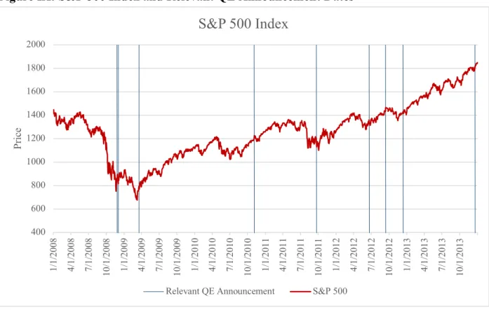
Figure IX: S&P 500 Index and Relevant QE Announcement Dates

30 _{Model 2 has an R-Squared value of 0.988 compared to 0.981 for Model 1 confirming our belief} that Model 2 is the relevant model for analysis of the equity market. Both Models 2 and 3 have the same R-Squared values, however, Model 2 has more statistical significance of each variable and a slightly lower Root MSE value (25.888 vs. 25.896).

400 600 800 1000 1200 1400 1600 1800 2000 1/ 1/ 2008 4/ 1/ 2008 7/ 1/ 2008 10/ 1/ 200 8 1/ 1/ 2009 4/ 1/ 2009 7/ 1/ 2009 10/ 1/ 200 9 1/ 1/ 2010 4/ 1/ 2010 7/ 1/ 2010 10/ 1/ 201 0 1/ 1/ 2011 4/ 1/ 2011 7/ 1/ 2011 10/ 1/ 201 1 1/ 1/ 2012 4/ 1/ 2012 7/ 1/ 2012 10/ 1/ 201 2 1/ 1/ 2013 4/ 1/ 2013 7/ 1/ 2013 10/ 1/ 201 3 Pr ic e

S&P 500 Index

Figure X: S&P 500 Index * p<0.05, ** p<0.01, *** p<0.001 p-values in parentheses R-sq 0.981 0.988 0.988 N 1494 1494 1493 _cons 2.035 (0.664) 4654.6*** (0.000) 4690.4*** (0.000) DlyGrw~rWeek 6.302 (0.484) VIXIndex -3.407*** (0.000) -3.425*** (0.000) RealGDP 0.000811*** (0.000) 0.000817*** (0.000) CorePCE -42.06*** (0.000) -42.43*** (0.000) U6 -10.35*** (0.000) -10.35*** (0.000) SP500_Prio~k 0.999*** (0.000) 0.734*** (0.000) 0.734*** (0.000) RelevantQE~s 20.60 (0.065) 18.82* (0.031) 19.05* (0.029) Model 1 Model 2 Model 3.2 S&P 500 1-Day * p<0.05, ** p<0.01, *** p<0.001 p-values in parentheses R-sq 0.981 0.989 0.989 N 1489 1489 1489 _cons -0.0893 (0.985) 4808.0*** (0.000) 4810.7*** (0.000) DlyGrwthT~ly 0.870 (0.922) VIX_1Week -3.503*** (0.000) -3.505*** (0.000) RealGDP_1W~k 0.000830*** (0.000) 0.000830*** (0.000) CorePCE_1W~k -43.72*** (0.000) -43.75*** (0.000) U6_1Week -9.803*** (0.000) -9.805*** (0.000) SP500_Prio~k 0.0961*** (0.000) 0.169*** (0.000) 0.168*** (0.000) SP500 0.905*** (0.000) 0.570*** (0.000) 0.570*** (0.000) RelevantQE~s 16.97 (0.128) 23.00** (0.007) 23.02** (0.007) Model 1 Model 2 Model 3.2 S&P 500 1-Week * p<0.05, ** p<0.01, *** p<0.001 p-values in parentheses R-sq 0.948 0.982 0.982 N 1479 1479 1479 _cons 3.753 (0.634) 7966.0*** (0.000) 7985.7*** (0.000) DlyGrw~1Week 14.16 (0.219) VIX_1Month -5.840*** (0.000) -5.888*** (0.000) RealGDP_1M~h 0.00137*** (0.000) 0.00137*** (0.000) CorePCE_1M~h -72.81*** (0.000) -73.00*** (0.000) U6_1Month -14.93*** (0.000) -14.97*** (0.000) SP500_1Week 0.946*** (0.000) 0.370*** (0.000) 0.372*** (0.000) SP500 0.0551 (0.201) 0.214*** (0.000) 0.212*** (0.000) RelevantQE~s 15.00 (0.442) -5.222 (0.648) -4.822 (0.673) Model 1 Model 2 Model 3 S&P 500 1-Month

Given that a Relevant QE announcement is likely to be perceived by the market as a positive, expansionary signal from the FOMC, a statistically significant positive increase in the price of the S&P 500 in the short-run should be the result. As we anticipated, in the short-term there is a statistically significant effect. Our model estimates a $19.05 increase in the price of the S&P 500 – significant at the 5% level (see Figure XI). However, as was observed in the yield on the BAML BBB index, changes in the VIX Volatility Index play a more significant role in the pricing of the equity market than QE announcements do. Relevant QE announcements have the strongest and most significant effect during time period 2. Here, our model estimates a $23.02 increase (significant at the 1% level) in the S&P 500 a week after a relevant QE announcement has occurred. This confirms that LSAPs did have some roll-over effect on the prices of equities – at least in the short- to medium- term.

When assessing the longer-term adjustments in the macro-economy and the financial markets, however, this effect has faltered. In the third time period, Model (2) estimates that a relevant QE announcement one month prior will result in a $4.82 decrease in the price of the S&P 500. That said, this decrease is a very statistically insignificant result – it has a p-value of 0.673 – with a p-value this high, it is likely that the actual effect is zero. To that end it can be concluded that any initial effects of LSAPs on the price of the equities as measured by the S&P 500 Index are unsustainable.

V. Conclusion

The effectiveness of Quantitative Easing as a non-conventional monetary policy instrument and its effect on the prices and yield of financial assets has been discussed and debated since its initial use nearly ten years ago. Consideration of the FOMC’s employment of QE policy cannot

be complete without thorough analysis of both its short- and longer-term effects in the financial markets. Our analysis extended previous work into the longer-term and adds additional assets classes to consideration. We find that in the short-term, the FOMC’s QE program did have a significant impact in the financial markets via the Portfolio Balance Effect. This initial effect was greatest on 30-Year Mortgage-Backed Securities and on the 10-Year Treasury Note – two of the largest asset classes purchased by the FOMC throughout the duration of their LSAPs.

This impact did not last in strength and significance as time passed, allowing for the financial markets to adjust to a new normal. As is consistent with our hypothesis, the effect of QE on prices and yields became insignificant on every asset class considered. This is not to say that QE was an ineffective and pointless program. Rather, our conclusion is that Quantitative Easing as a form of monetary policy lacks the long-run sustainability that is necessary to be a fully effective instrument of monetary policy.

References

Bernanke, Ben S., Vincent R. Reinhart, and Brian P. Sack. 2004. “Monetary Policy Alternatives at the Zero Bound: An Empirical Assessment.” Brookings Papers on Economic Activity 2004(2) 1-78.

Breedon, Francis, Jagjit S. Chadha, and Alex Waters. 2012. “The financial market impact of UK quantitative easing.” Oxford Review of Economic Policy 28(4) 702-728

D’Amico, Stefania and Thomas B. King. 2013. “Flow and stock effects of large-scale treasury purchases: Evidence on the importance of local supply.” Journal of Financial Economics 2013 425-448.

The Economist. “The Bank of Japan sticks to its guns.” September 30, 2017.

Engen, Eric M., Thomas Laubach, and David Reifschneider. “The Macroeconomic Effects of the Federal Reserve’s Unconventional Monetary Policies.” Finance and Economics Discussion Series, Federal Reserve Board, Washington, D.C., January 14, 2015.

Eser, Fabian and Bernd Schwaab. “Evaluating the impact of unconventional monetary policy measures: Empirical evidence from the ECB’s Securities Markets Program.” Journal of Financial Economics. 119 (2016) 147-167.

Federal Reserve Board. Addendum to the Policy Normalization Principle and Plans. June 14, 2017. https://www.federalreserve.gov/newsevents/pressreleases/monetary20170614c.htm

–––––. FOMC Statement. Press release, December 16, 2008.

https://www.federalreserve.gov/newsevents/pressreleases/monetary20081216b.htm

–––––. FOMC Statement. Press release, September 13, 2012.

–––––. FOMC Statement. Press release, December 12, 2012. https://www.federalreserve.gov/newsevents/pressreleases/monetary20121212a.htm

–––––. FOMC Statement. Press release, December 18, 2013.

https://www.federalreserve.gov/newsevents/pressreleases/monetary20131218a.htm

–––––. FOMC Statement. Press release, September 20, 2017.

https://www.federalreserve.gov/newsevents/pressreleases/monetary20170920a.htm Gagnon, Joseph, Matthew Rasking, Julie Remache, et.al. 2011. “The Financial Market Effects of

the Federal Reserve’s Large-Scale Asset Purchases.” International Journal of Central Banking 7(1) 3-43.

Gagnon, Joseph E. “Quantitative Easing: An Underappreciated Success.” Policy Brief No. PB16-4. Peterson Institute for International Economics, Washington, D.C. (April 2016)

Glick, Reuven and Sylvain Leduc. 2012, “Central bank announcements of asset purchases and the impact on global financial and commodity markets.” Journal of International Money and Finance 31 2078-2101.

Greenlaw, David, James D. Hamilton, Ethan S. Harris, and Kenneth D. West. 2018. “A Skeptical View of the Impact of the Fed’s Balance Sheet.” US Monetary Policy Forum. February 2018. https://research.chicagobooth.edu/igm/usmpf/usmpf-paper

Harrison, David. “Fed Officials Split Over Timing of Next Rate Increase.” The Wall Street Journal. August 16, 2017.

Joyce, Michael A.S., Ana Losaosa, Ibrahim Stevens, et.al. 2011. “The Financial Market Impact of Quantitative Easing in the United Kingdom.” International Journal of Central Banking. 7(3) 113-161.

Krishnamurthy, Arvind and Annette Vissing-Jorgensen. 2011. “The Effects of Quantitative Easing on Interest Rates: Channels and Implications for Policy.” Brookings Papers on Economic Activity Fall 2011 215-287.

Partington, Richard. “ECB to halve bond buying as it plans to scale back quantitative easing.” The Guardian, October 26, 2017. https://www.theguardian.com/business/2017/oct/26/ecb-to-halve-bond-buying-as-it-plans-to-scale-back-quantitative-easing

Rosengren, Eric S. “Lessons from the U.S. Experience with QE.” Presentation at the Joint Even on Sovereign Risk and Macroeconomics, Frankfurt, Germany, February 5, 2015.

Swanson, Eric T. 2017. “Measuring the Effects of Federal Reserve Forward Guidance and Asset Purchases on Financial Markets.” NBER Working Paper 23311. National Bureau of Economic Research, Cambridge, MA.

Appendix

Appendix Figure I: Bank of England Balance Sheet

Data Source: Bank of England

Appendix Figure II: European Central Bank Balance Sheet

Data Source: European Central Bank 0 100 200 300 400 500 2007 2008 2009 2010 2011 2012 2013 2014 GBP ( bi lli on s) Year

Bank of England Balance Sheet Assets 2007-2014

Other assets including loan to the Asset Purchase facility £ Ways and means advances to HM government

Central Bank bonds and other securities acquired via market transactions £ long-term operations with BoE

£ Short-term repo operations with BoE

0 500000 1000000 1500000 2000000 2500000 10/ 01 /14 12/ 01 /14 02/ 01 /15 04/ 01 /15 06/ 01 /15 08/ 01 /15 10/ 01 /15 12/ 01 /15 02/ 01 /16 04/ 01 /16 06/ 01 /16 08/ 01 /16 10/ 01 /16 12/ 01 /16 02/ 01 /17 04/ 01 /17 06/ 01 /17 08/ 01 /17 10/ 01 /17 12/ 01 /17 Eu ro ( m ill io ns ) Date

ECB Asset Purchase Program 2014-2018

Asset-backed securities purchase programme Covered bond purchase programme 3 Corporate Sector purchase programme Public sector purchase programme