Decomposition-Based-Sorting and
Angle-Based-Selection for Evolutionary
Multiobjective and Many-Objective Optimization
Xinye Cai, Member, IEEE, Zhixiang Yang, Zhun Fan, Senior Member, IEEE,
and Qingfu Zhang, Senior Member, IEEE
Abstract—Multiobjective evolutionary algorithm based on decomposition (MOEA/D) decomposes a multiobjective optimiza-tion problem (MOP) into a number of scalar optimizaoptimiza-tion subproblems and then solves them in parallel. In many MOEA/D variants, each subproblem is associated with one and only one solution. An underlying assumption is that each subproblem has a different Pareto-optimal solution, which may not be held, for irregular Pareto fronts (PFs), e.g., disconnected and degener-ate ones. In this paper, we propose a new variant of MOEA/D with sorting-and-selection (MOEA/D-SAS). Different from other selection schemes, the balance between convergence and diversity is achieved by two distinctive components, decomposition-based-sorting (DBS) and angle-based-selection (ABS). DBS only sorts L closest solutions to each subproblem to control the convergence and reduce the computational cost. The parameter L has been made adaptive based on the evolutionary process. ABS takes use of angle information between solutions in the objective space to maintain a more fine-grained diversity. In MOEA/D-SAS, differ-ent solutions can be associated with the same subproblems; and some subproblems are allowed to have no associated solution, more flexible to MOPs or many-objective optimization problems (MaOPs) with different shapes of PFs. Comprehensive experi-mental studies have shown that MOEA/D-SAS outperforms other approaches; and is especially effective on MOPs or MaOPs with
Manuscript received January 5, 2016; revised May 25, 2016; accepted June 15, 2016. This work was supported in part by the National Natural Science Foundation of China under Grant 61300159, Grant 61473241, Grant 61332002, Grant 61370185 and Grant 61175073, in part by the Natural Science Foundation of Jiangsu Province of China under Grant BK20130808, in part by the China Post-Doctoral Science Foundation under Grant 2015M571751, in part by the Science and Technology Planning Project of Guangdong Province of China under Grant 2013B011304002, in part by the Educational Commission of Guangdong Province of China under Grant 2015KGJHZ014, in part by the Fundamental Research Funds for the Central Universities of China under Grant NZ2013306, and in part by the Guangdong High-Level University Project “Green Technologies” for Marine Industries. This paper was recommended by Associate Editor G. G. Yen.
X. Cai and Z. Yang are with the College of Computer Science and Technology, Nanjing University of Aeronautics and Astronautics, Nanjing 210016, China (e-mail:[email protected];[email protected]).
Z. Fan is with the Guangdong Provincial Key Laboratory of Digital Signal and Image Processing and the Department of Electronic Engineering, School of Engineering, Shantou University, Shantou 515063, China (e-mail: [email protected]).
Q. Zhang is with the Department of Computer Science, City University of Hong Kong, Hong Kong, and also with the School of Computer Science and Electronic Engineering, University of Essex, Colchester CO4 3SQ, U.K. (e-mail:[email protected]).
This paper has supplementary downloadable multimedia material available athttp://ieeexplore.ieee.orgas a PDF file provided by the authors. The total size of the file is 414 KMB in size.
Color versions of one or more of the figures in this paper are available online athttp://ieeexplore.ieee.org.
Digital Object Identifier 10.1109/TCYB.2016.2586191
irregular PFs. Moreover, the computational efficiency of DBS and the effects of ABS in MOEA/D-SAS are also investigated and discussed in detail.
Index Terms—Angle-based-selection (ABS), decomposition-based-sorting (DBS), diversity, evolutionary multiobjective opti-mization, many-objective optimization.
I. INTRODUCTION
M
ULTIOBJECTIVE optimization problems (MOPs) involve the optimization of more than one objective function. Since these objectives usually conflict with each other, no single optimal solution exists to optimize all the objectives simultaneously. Instead, Pareto-optimal solutions, which are their best tradeoff candidates, can help decision makers to understand the tradeoff relationship among different objectives and choose their preferred solutions. In the field of multiobjective optimization, the set of all the Pareto-optimal solutions is usually called the Pareto set (PS) and the image of (PS) on the objective vector space is called the Pareto front (PF) [30]. Over the past decades, multiobjective evolu-tionary algorithms (MOEAs) have been recognized as a major methodology for approximating the PF [5], [9], [10], [12], [18], [36]–[38].In MOEAs, selection is of great importance for the perfor-mance of MOEAs. Usually, it is desirable to balance between convergence and diversity for obtaining good approximation to the set of Pareto-optimal solutions [4], [17]. Convergence can be measured as the distance of solutions toward the PF, which should be as small as possible. Diversity can be mea-sured as the spread of solutions along the PF, which should be as uniform as possible.
Based on the above two requirements for selec-tion, the current MOEAs can be categorized into the domination-based (see [15], [42], [44]), the indicator-based (see [2], [3], [24], [43]), and the decomposition-indicator-based MOEAs (see [20], [21], [35], [40]). A representative of decomposition-based MOEAs is MOEA based on decompo-sition (MOEA/D) [40], which can be regarded as a general-ization of cMOGA [31]. MOEA/D decomposes an MOP into a number of single objective optimization subproblems and then solves them in parallel. The objective function in each subproblem can be a linear or nonlinear weighted aggregation function of all the objective functions in the MOP in question. 2168-2267 c2016 IEEE. Personal use is permitted, but republication/redistribution requires IEEE permission.
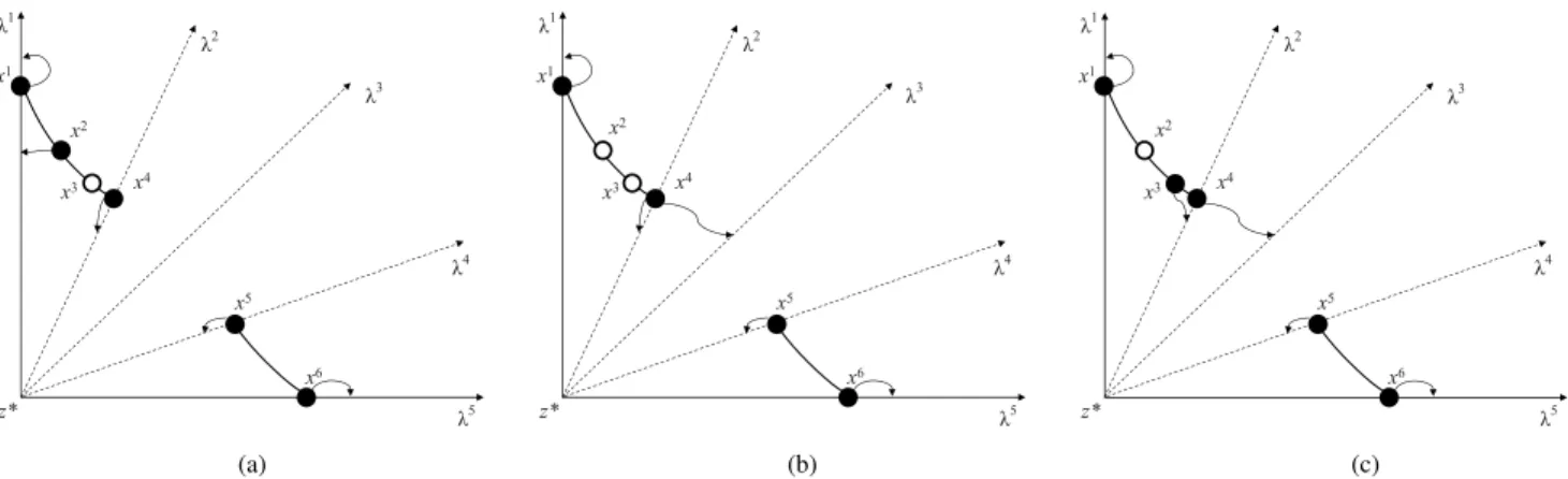
Fig. 1. Illustrative examples of different selection results. (a) Ideal selection result. Selection result obtained by (b) MOEA/D and (c) MOEA/D-STM.
In MOEA/D, each solution is associated with a subproblem, and two subproblems are called neighbors if their weight vectors are close to each other. MOEA/D explores correla-tion relacorrela-tionships among neighboring subproblems to speed up its search. The diversity is implicitly achieved by speci-fying a wide spread of the directions in the objective space. Several variants of MOEA/D have been proposed and studied (see [1], [6], [7], [19], [23], [26], [28], [29], [39]). For exam-ple, an online geometrical metric was proposed to enhance the diversity of MOEA/D in [19]. In [28], a global stable matching (STM) model is integrated into MOEA/D for suitable matches between subproblems and solutions. In MOEA/D-STM, each subproblem prefers the solution with better aggregation func-tion value, which indicates a better convergence along its search direction. Therefore, the preferences of subproblems encourage convergence. Meanwhile, each solution agent ranks all subproblems according to its distance to the weight vec-tor of these subproblems. Therefore, the preferences of the solutions can promote the diversity. The STM between sub-problems and solutions achieves an equilibrium between their mutual-preferences and thus, a balance between convergence and diversity can be achieved.
The motivations of this paper are based on the following considerations.
1) In many MOEA/D variants, e.g., MOEA/D-STM, each subproblem is allowed to associate with one and only one solution. An underlying assumption is that each subproblem leads to a diversely located Pareto opti-mal solution in PF. It could hold if the weight vectors of the subproblems are appropriately assigned priori. However, for the real-world MOPs, both shape and spread of the PFs are unknown and this assumption is not likely to be held, especially for disconnected and degenerate PFs [22]. Fig. 1 shows the ideal selection results for such a PF as well as the ones obtained by MOEA/D and MOEA/D-STM. The population diversity for both MOEA/D and MOEA/D-STM has not been well-maintained due to the above assumption. Under this circumstance, it is not reasonable to force one subprob-lem to associate with one solution. The framework of MOEA/D can be more flexible to accommodate MOPs with different shapes of PFs.
2) As a state-of-the-art variant of MOEA/D, MOEA/D-STM can usually, achieve good balance between the convergence and diversity. However, the computational cost of its selection scheme is still high [O(NM log M), where N is the population size and M is 2*N], due to the use of global STM model.1 The selection of local solutions for each subproblem can be used to reduce the computational complexity.
3) Although some advanced diversity maintenance schemes, e.g., niche-counts [14], have been adopted for MOEA/D to further increase its diversity [27]. Nevertheless, such scheme is, in some sense, very coarse-grained: it does not distinguish subproblems with the same niche-counts and it is possible that solutions associated with different subproblems may be close to each other while solutions associated with the same subproblems may be far from each other. To further increase the diversity, a more fine-grained diversity maintenance scheme is desired.
Based on the above considerations, this paper pro-poses a new variant of MOEA/D with sorting-and-selection (MOEA/D-SAS) for MOPs. Different from other selection schemes, the balance between convergence and diver-sity is achieved by two distinctive components, decomposition-based-sorting (DBS) and angle-based-selection (ABS). DBS only sorts L closest solutions to each subproblem to con-trol the convergence and reduce the computational cost. The parameter L has been made adaptive based on the evolutionary process. ABS takes use of angle information between solutions in the objective space to maintain a more fine-grained diver-sity. In addition, different solutions can be associated with the same subproblems; and some subproblems are allowed to have no associated solution, which is more flexible to MOPs with different shapes of PFs.
The rest of this paper is organized as follows. Section II introduces some preliminaries on multiobjective optimization and decomposition methods. Section III describes the pro-posed sorting-and-selection (SAS) scheme, which contains two important components, DBS and ABS. In Section IV,
1Most high computational cost originates from sorting for the preference
SAS is integrated into MOEA/D. Section V introduces the benchmark test functions and the performance indica-tors used in this paper. Experimental studies and discussion are presented in Section VI, where we compare our pro-posed algorithm with four classical MOEAs: 1) NSGA-II; 2) MOSOPS-II; 3) MOEA/D; and 4) MOEA/D-DE; and three state-of-the-art MOEA: 1) MOEA/D-STM; 2) NSGA-III; and 3) MOEA/D-AWA on MOPs or many-objective optimization problem (MaOPs). The effects of DBS and ABS are also inves-tigated and discussed in Section VI. Section VII concludes this paper.
II. PRELIMINARIES
This section first gives some basic definitions of multiob-jective optimization. Then, some basic knowledge about the decomposition methods used in this paper is also introduced.
A. Basic Definitions
An MOP can be defined as follows:
minimize F(x)=(f1(x), . . . ,fm(x))T
subject to x∈ (1)
where is the decision space, F : → Rm consists of m real-valued objective functions. The attainable objective set is
{F(x)|x∈}.
Let u,v∈Rm, u is said to dominate v, denoted by u≺ v,
if and only if ui ≤ vi for every i ∈ {1, . . . ,m} and uj <vj
for at least one index j ∈ {1, . . . ,m}.2 A solution x∗ ∈ is Pareto-optimal to (1) if there exists no solution x∈such that
F(x) dominates F(x∗). F(x∗) is then called a Pareto-optimal (objective) vector. In other words, any improvement in one objective of a Pareto-optimal solution is bound to deteriorate at least another objective.
B. Decomposition Methods
In principle, many methods can be used to decompose an MOP into a number of scalar optimization subproblems [30]. Among them, the most popular ones are weighted sum (WS), Tchebycheff (TCH), and penalty boundary intersection (PBI) approaches [40]. The mathematical definition of these decom-position methods are as follows.
1) WS Approach: This approach considers a convex com-bination of all the objectives. One single objective subproblem sk is defined as minimize gws x|λk = m i=1 λk ifi(x) subject to x∈ (2)
whereλk =(λk1, . . . , λkm)T is the direction vector of
sub-problem sk, and λki ≥0, i∈1, . . . ,m andmi=1λki =1. The optimal solution to (2) is a Pareto-optimal solution to (1). A set of different Pareto-optimal solutions can be obtained simply by using different direction vectors, to approximate the PF when it is convex.
2In the case of maximization, the inequality signs should be reversed.
2) TCH Approach: In this approach, one single objective subproblem sk is defined as minimize gte x|λk,z∗ = max 1≤i≤m |fi(x)−z∗i|/λki subject to x∈ (3)
z∗ = (z∗1, . . . ,z∗m)T is the ideal objective vector, where
z∗i < min{fi(x)|x∈ }, i ∈ 1, . . . ,m. For convenience, λk
i =0 is replaced byλki =10−6, becauseλki =0 is not
allowed as a denominator in (3).
3) PBI Approach: This approach is a variant of normal-boundary intersection approach [11]. A subproblem sk is defined as minimize gpbi x|λk,z∗ =d1+βd2 d1= F(x)−z∗ Tλk/||λk|| d2= ||F(x)−z∗− d1/||λk|| λk|| subject to x∈ (4)
where ||.|| denotes the L2-norm, and β is the penalty parameter.
III. SELECTIONOPERATORS
This section elaborates the selection operator based on the DBS and the ABS (SAS) scheme.
Given a set of N subproblems S and a set of M solutions,
Z, the goal of SAS is to select N solutions from Z to form P.
For each subproblem j that has a direction vectorλj, Pj(L)
denotes the set of the first L closest solutions toλj in Z. The “closeness” is defined by the acute angle between the solution
x and the direction vectorλj, based on anglex, λj =arccos (F(x)−z∗)Tλj F(x)−z∗ λj . (5)
The input parameter L in the current call of SAS has been adaptive, based on the value of outputαin the previous call of SAS (see step 3 of Algorithm 4). L is defined as the number of closest solutions to each subproblem and α is the number of selected solution sets, which is explained in Section III-A.
A. Framework of SAS
The pseudo-code of SAS is presented in Algorithm 1.
1) Sorting: In step 1, P is first initialized to be an
empty set. The DBS is conducted iteratively. DBS, presented in Algorithm 2, is detailed in Section III-B. In the ith iteration of DBS, L solution sets (fronts) Q(i−1)∗L+1, . . . ,
Q(i−1)∗L+j, . . . ,Qi∗L can be obtained by sorting population
Z (or part of the population Z, depending on the value of L).
Then, these sorted solution sets are added to P and eliminated from Z (lines 5–8). This process is repeated until the total number of sorted solutions|P|exceeds the population size N. After step 1, the population Z (or part of the population Z) is divided into L∗(i−1)solution sets (fronts): Q1, . . . ,QL∗(i−1), where i−1 is the total number of iterations of DBS and L is the number of closest solutions in the population Z to each subproblem. Note that possible overlapped solutions may exist
Algorithm 1: SAS(Z,z∗,L,N)
Input:
1) Z: the solution set;
2) z∗: the ideal objective vector;
3) L: the number of closest solutions to each subproblem;
4) N: the size of P.
Output:
1) the population P;
2) the number of selected frontsα.
Step 1 Sorting: 1 P= ∅; 2 i=1; 3 do 4 [Q(i−1)∗L+1, . . . ,Qi∗L] = DBS (Z,z∗,L); 5 for k=(i−1)∗L+1 to i∗L do 6 P=PQk; 7 Z =Z\Qk; 8 end 9 i=i+1; 10 while |P|<N; Step 2 Selection: 11 P= ∅; 12 k=1; 13 while |PQk| ≤N do 14 P=PQk; 15 k=k+1; 16 end 17 if |PQk|>N then 18 A=Qk\P; 19 P=ABS(A,P,z∗,N); 20 α=k; 21 else 22 α=k−1; 23 end 24 return P and α;
in different fronts Qk. The value of i (2 ≤ i ≤ (N+1)) is determined by both value of L (1≤L≤ |Z|) and evolutionary status of the algorithm. However, two extreme cases in terms of the value of L can be analyzed as follows. When L =1, only the closest solution to each subproblem is chosen, which indicates only the solution closest to the direction vector of each subproblem gets involved in sorting. In this case, the diversity is emphasized and DBS is conducted for multiple times (i>2). When L= |Z|, the whole population Z is sorted for every subproblem and Z is divided into at most|Z|fronts. In this case, convergence is emphasized and DBS is conducted for only one time (i = 2). Therefore, more convergence is likely to be emphasized with the increase of the value of L.
2) Selection: In step 2, N solutions are selected out of the L∗(i−1)solution sets (fronts) obtained from step 1, as follows.
P is initialized to be an empty set. For the kth front, if the
size of the combined set (P∪Qk) is smaller than N, then Qk is added to P and the remaining members of P are chosen
Algorithm 2: DBS(Z,z∗,L)
Input:
1) Z: the solution set;
2) z∗: the ideal objective vector;
3) L: the number of closest solutions to each subproblem. Output: 1) L solution sets: Q1, . . . ,QL; 1 Q1=Q2=. . .=QL = ∅. 2 for j=1 to N do 3 Pj(L)=Associate(Z, λj); /* Associate
subproblem j with the L closest
solutions Pj in Z, based on (5). */
4 for k=1 to L do
5 g(Pj(k)|λj,z∗); /* Computing the
aggregation function values. */
6 end
7 Pj=Sort(Pj); /* Sort Pj in an ascending
order, based on g(Pj|λj,z∗) values. */
8 end 9 for k=1 to L do 10 for j=1 to N do 11 Qk=Qk{Pj(k)}; 12 end 13 end 14 return Q1, . . . ,QL ;
from Qk+1. This procedure is continued until no more sets can be accommodated (lines 13–16). If the size of the com-bined set (P∪Qk) is larger than N and say that the set Qα is the last set beyond which no other set can be accommodated. Then the previously selected solutions in P are eliminated from
Qα (Qα\P) and stored in an intermediate set A. The ABS is
activated to select solutions from A to fill P. More details of ABS are presented in Algorithm 3 in Section III-C. The number of actually selected sets (Q1, . . . ,Qα) is saved asα.
3) Termination: The solution set P and α are returned as the outputs.
B. Decomposition-Based-Sorting
The detailed procedures of DBS is presented in Algorithm 2 as follows. At the beginning, each subproblem j chooses its closest L solutions Pj in Z, based on (5) (line 3). The chosen solutions are sorted into L solution sets (fronts),
Q1, . . . ,Qk, . . . ,QL (lines 9–13), where Qkcontains the solu-tions with the kth best g(∗|λj,z∗) values, in Pj for every subproblem j, (1 ≤ j ≤ N) (lines 4–7). Note that it is
pos-sible that|Qk| ≤N since two different subproblems may have
the same kth best solution in Qk. An illustrative example of DBS can be found in Section I of supplementary material.
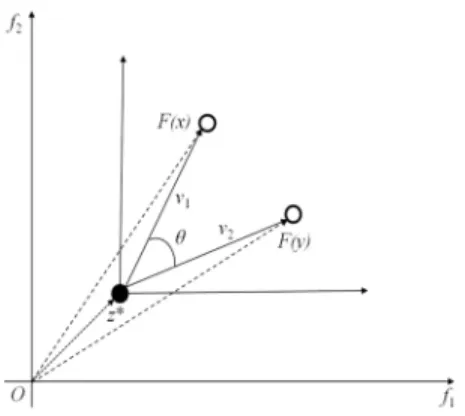
C. Angle-Based-Selection
To further improve the diversity in the population, our selec-tion scheme needs to consider the diversity relaselec-tionship between the selecting solutions and the solutions in the previously
Fig. 2. Illustration of the angle between solution x and y.
Algorithm 3: ABS(A,P,z∗,N)
Input: two populations A and P, the ideal objective
vector z∗, size of P: N
Output: the population P
1 foreach xi∈A do 2 θi←minxj∈P{angle(xi,xj)}; 3 end 4 for i←1 to |A|do 5 k←argmaxk{θk}; 6 if |P|<N then 7 A←A\ {xk}; 8 θ ←θ\ {θk}; 9 P←P{xk}; 10 foreach xj∈A do 11 θj←min{θj,angle(xk,xj)}; 12 end 13 else 14 break; 15 end 16 end 17 return P;
selected fronts. In this paper, we use acute angles between objective vectors of solutions to quantify diversity, as follows:
angle(x,y)=arccos vT1v2 v1 v2 (6) where v1=F(x)−z∗ v2=F(y)−z∗.
F(x)and F(y)are, respectively, the objective vectors of solu-tion x ∈ P and y ∈ A, and z∗ is the ideal objective vector. Fig. 2 shows the calculation of diversity, as presented in (6). The idea of ABS is that, a member is added to P if and only if its angle with elements in P is the largest.
The pseudo-code of ABS is presented in Algorithm 3. For each solution xi∈A in the selecting front, its minimum angle,
θi, to each solution in P, is calculated (lines 1–3), based on (6).
To maximize the diversity, line 5 obtains the solution (xk) with the largest angle (θk) to P. If the size of P is less than N,
it will be deleted from A and added to P (lines 7–9); and the corresponding minimum angle between xj and P is updated (lines 10–12); otherwise, the loop is terminated. Finally, P is returned as the output (line 17). An illustrative example of ABS can be found in Section II of supplementary material.
D. Computational Cost of the SAS
In DBS (Algorithm 2), the computational cost of associa-tion operators (N cycles of line 3) for all the subproblems can be easily reduced by the following two steps. The first step approximates the objective vectors of all the solutions in Z to their closest direction vectors, which requires O(mM) compu-tations, where m is the number of objectives and M=2N is the size of population Z. The second step needs O(L) compu-tations to obtain L neighboring solutions for each subproblem based on the first step. Therefore, the total computational cost of association operators for all the subproblems can be reduced to O(LN). The complexity to calculate g(∗)for all the sub-problems is O(mLN) (N cycles of lines 4–6). O(NL log L)
comparisons are used to sort g(∗)values (N cycles of line 7). So the complexity of Algorithm 2 is the larger one of O(mLN)
and O(NL log L).
In ABS (Algorithm 3), the computational cost can also be reduced if each solution in A only calculates its angle to each solution xiin S⊂P, where S is T |P|neighboring solutions of xi∈ P. Suppose that the size of solution set A is Na. The
calculation of minimum angles between each solution in A and S (lines 1–3) needs O(mNaT) computations. The cycles
from lines 4–16 are executed at most Na times. Line 11 is
executed Na∗(Na−1)/2 times. Therefore, in the worst case,
the complexity of Algorithm 3 is O(Na2)(NaN).
In SAS (Algorithm 1), at most N solutions are added to
P in step 2, so the computational cost of for-loop in step 1
is O(N log N). The computational cost of DBS in step 1 is O(mLN) or O(NL log L). At most N solutions are added to P in step 2, so the computational cost of while-loop in step 2 is also O(N log N). ABS in step 2 needs O(NaNa)
(NaN). So the computational cost of the SAS is the larger
one of O(mLN), O(NL log L) (L N) and O(N log N). On the contrary, the computational cost of the STM model is
O(NM log M). Apparently, either one of O(mLN), O(NL log L), and O(N log N) is much smaller than O(NM log M) and the computational complexity of SAS has been greatly reduced compared with STM.
IV. INTEGRATION OFSAS WITHMOEA/D In this section, SAS is integrated into MOEA/D. The pseudo-code of our algorithm, called MOEA/D-SAS, is demonstrated in Algorithm 3.
At each generation, MOEA/D-SAS maintains the following. 1) A population of N solutions, P= {x1, . . . ,xN}.
2) A set of N subproblems, S= {s1, . . . ,sN}.
3) Objective function values, FV1, . . . ,FVN, where FVi is the F-value of xi.
The algorithm works as follows. Step 1: Initialization: Initialize P.
Algorithm 4: MOEA/D-SAS Input:
1) MOP(1);
2) a stopping criterion;
3) N: the number of subproblems; the population size of
P and Y;
4) λ1, . . . ,λN: a set of N weight vectors;
5) T: the size of the neighborhood for each subproblem.
Output: population P. Step 1 Initialization:
a) Compute the Euclidean distances between any two
weight vectors and obtain T closest weight vectors to each weight vector. For each i=1, . . . ,N, set
B(i)= {i1, . . . ,iT}where λi1, . . . , λiT are the T closest
weight vectors toλi.
b) Generate an initial population P= {x1, . . . ,xN}
randomly.
c) Initialize z∗=(z∗1, . . . ,z∗m)T by setting
z∗i =min{fi(x1), . . . ,fi(xN)}.
d) Initializeα=2∗N.
Step 2 New Solution Generation:
For each i=1, . . . ,|P|, do:
a) Selection of the Mating Solutions:
1) Associate each solution xi with its closest
subproblem k based on (5).
2) If rand(0,1) < δ, then set D to the set of solutions associated with all the subproblems in B(k), else, set D=P.
b) Reproduction: Set xr1 =xi and randomly select two
indices r2 and r3 from D, and then generate a new solution yi from xr1, xr2 and xr3 by DE.
c) Evaluation yi : FVi=F(yi).
d) Update of z∗ : For each j=1, . . . ,m, if zj∗>fj(yi),
then set z∗j =fj(yi).
Step 3 Sorting-and-Selection: Set L=min{α+T,2N},
[P, α] = SAS(PY,z∗,L,N).
Step 4 Stopping Criteria: If stopping criteria is satisfied,
then stop and output P. Otherwise, go to Step 2.
Step 2: New Solution Generation: Generate a set of new solutions Y.
Step 3: Sorting and Selection: Use Y to update P. Step 4: Stopping Condition: If a preset stopping condition
is met, output P. Otherwise, go to step 2.
The pseudocode of MOEA/D-SAS is given in Algorithm 4. The details of steps 1–3 are given as follows.
A. Initialization
MOEA/D-SAS decomposes an MOP into N single objective optimization subproblems by using a decomposition approach (WS, TCH, or PBI) with N weight vectors
λk=λk
1, . . . , λkm
T
k=1, . . . ,N (7) where λk ∈ Rm+ and im=1λki = 1. The subproblem sk is
defined by (2), (3), or (4), in Section II-B.
For each k =1, . . . ,N, let B(k) be the set containing the indices of the T closest weight vectors to λk in terms of the Euclidean distance. If i ∈ B(k), subproblem i is called a neighbor of subproblem k.
Solution xi in P can be generated randomly or by using a single objective heuristic on the subproblem i. The ideal objective vector is initialized as the minimum values of all the solutions in P along each objective.αis initialized as 2N.
B. New Solution Generation
An offspring population Y (size of N) is generated in step 2. For each solution xi in P, the process for generating a new solution yi is as follows.
In step 2a, the mating pool D for solution xi is set to the set of solutions associated with all the subproblems in B(k)
with probabilityδ or the population P with probability 1−δ. In step 2b, an offspring solution is reproduced, using par-ent solutions from the mating pool D. Any genetic operator or mathematical programming technique can serve this pur-pose, although differential evolution (DE) [32] and polynomial mutation [13] are used in this paper. We set one parent solu-tion xr1 = xi. The other two parent solutions, xr2 and xr3, are randomly selected from mating pool D, for generating an offspring solution as follows:
yj= xr1 j +F× xr2 j −x r3 j , if rand≤CR or j=jrand xr1 j , otherwise (8) where j= 1, . . . ,n, rand∈ [0,1], jrand ∈ [1,n] is a random
integer uniformly generated from 1 to n; and CR and F are two control parameters.
The polynomial mutation operator is applied on y to generate y=(y1, . . . ,yn)T yj= yj+σj×(bj−aj), with probability pm yj, with probability 1−pm (9) with σj= (2×rand)η+11 −1, if rand<0.5 1−(2−2×rand)η+11, otherwise (10) where rand is a random number uniformly generated from [0,1]; the distribution index η and the mutation rate pm are
two control parameters; and ajand bjare the lower and upper
bounds of the jth decision variable.
In step 2c, the new solution yi is evaluated. The ideal objective vector z∗ is updated in step 2d. The procedure (steps 2a–2d) is repeated N times, so a population Y =
{y1, . . . ,yN}can be obtained.
C. Sorting-and-Selection
SAS is called to updated P, that is to select N solutions out of combined population P∪Y. The neighborhood size L
for sorting in SAS, is adaptively controlled by the number of selected fronts in the last call of SAS. The maximum value of
TABLE I
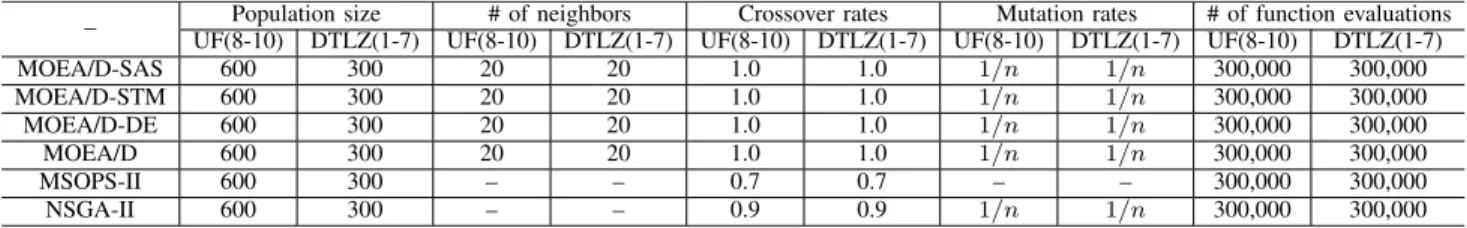
PARAMETERSETTINGS INMOEA/D-SAS, MOEA/D-STM, MOEA/D-DE, MOEA/D, MSOPS-II,ANDNSGA-IIFOR2-OBJECTIVETESTINSTANCES
TABLE II
PARAMETERSETTINGS INMOEA/D-SAS, MOEA/D-STM, MOEA/D-DE, MOEA/D, MSOPS-II,ANDNSGA-IIFOR3-OBJECTIVETESTINSTANCES
D. More Discussions on MOEA/D-SAS
In a very recent work [34], a decomposition-based MOEA (named WASF-GA) is proposed. In WASF-GA, the population is also divided into different fronts based on decomposition function values for subproblems. However, the selection of MOEA/D-SAS is fundamentally different from WASF-GA in the following two aspects.
1) MOEA/D-SAS can also deal with MOPs with irreg-ular PFs, e.g., the disconnected and degenerate ones. Therefore, for the same case in Fig.1, WASF-GA can only achieve the selection results in Fig. 1(b), while MOEA/D-SAS can achieve the ideal results in Fig.1(a), due to the following two distinctive characteristics of MOEA/D-SAS.
a) Different solutions are allowed to associate with the same subproblems and some subproblems may have no associated solutions.
b) ABS adopts the angle information to select solu-tions with the best diversity.
2) Different from WASF-GA, which conducts sorting on all the solutions for each subproblem, DBS only sorts
L closest solutions to each subproblem to control the
convergence and reduce the computational cost. V. EXPERIMENTALSETTING
A. Test Problems
Two well-known test suites are considered in our exper-imental studies. One is the UF test suite which contains ten unconstrained MOP test instances (UF1–UF10) from the CEC2009 MOEA competition [41]. Seven of them (UF1–UF7) are 2-objective test functions, and the rest (UF8–UF10) are 3-objective functions. For all UF test functions, the num-ber of decision variables is set to 30. Another test suite is DTLZ [16]. All DTLZ instances can be scaled to any number of objectives and decision variables. In this paper, the number
of objectives is set to 3 and the number of decision variables is set to 10.
B. Parameter Settings
All the algorithms were implemented in MATLAB. The parameters of NSGA-II, MSOPS-II, MOEA/D, MOEA/D-DE, and MOEA/D-STM were set according to [15], [20], [25], [28], and [40]. The parameters of MSOPS-II, MOEA/D, MOEA/D-STM, and MOEA/D-SAS were set in such a way that they shared the same key parameter values with MOEA/D-DE. Their parameter settings for 2- and 3-objective benchmark functions are listed in TablesIandII, respectively. The setting of N weight vectors (λ1, . . . , λN)is controlled by a positive integer parameter H, which specifies the granular-ity or resolution of weight vectors, as in [40]. Each individual weight takes a value from
0 H, 1 H, . . . , H H .
The number of weight vectors is determined by both parameter
H and the number of objectives m: N = CmH−+1m−1.
C. Performance Metrics
Inverted generational distance (IGD) [8], [45] is used as the performance metric in our studies. IGD measures the average distance from a set of reference points P∗ in the PF to the approximation set P. It can be formulated as follows:
IGD(P,P∗)= 1
|P∗|
v∈P∗
dist(v,P) (11) where dist(v,P)is the Euclidean distance between the solution
v and its nearest point in P, and|P∗|is the cardinality of P∗. If
|P∗|is large enough to represent the PF very well, IGD(P,P∗)
TABLE III
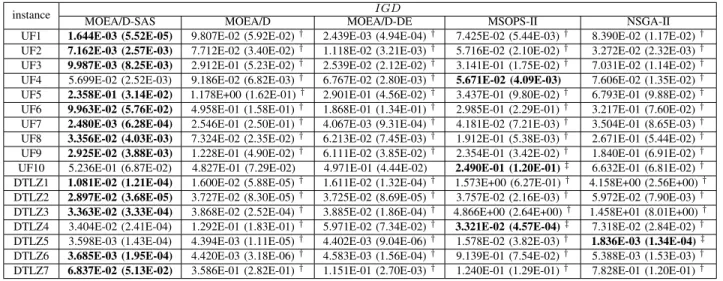
MEAN ANDSTANDARDDEVIATIONVALUES OFIGD, OBTAINED BYMOEA/D-SAS, MOEA/D, MOEA/D-DE, MSOPS-II,ANDNSGA-IIONUFANDDTLZ INSTANCES
VI. EXPERIMENTALSTUDIES ANDDISCUSSION To study the performance of MOEA/D-SAS and understand its behavior, this section conducts the following experimental works.
1) Comparisons of MOEA/D-SAS with NSGA-II [15], MOEA/D [40], MOEA/D-DE [25], and MSOPS-II [20]. 2) Comparisons of MOEA/D-SAS with
MOEA/D-STM [28].
3) Investigation of the computational efficiency of DBS. 4) Investigation of the effects of ABS in MOEA/D-SAS. In our experiments, each algorithm was run 30 times inde-pendently for each test instance. To make fair comparisons, TCH approach has been used as decomposition approach in MOEA/D, MOEA/D-DE, and MOEA/D-SAS on 2- or 3-objective optimization problems.
A. Comparisons With Classical MOEAs
In this section, we compare MOEA/D-SAS with four clas-sical domination or decomposition-based MOEAs—NSGA-II, MSOPS-II, MOEA/D, and MOEA/D-DE.
The performances of SAS, MOEA/D, MOEA/D-DE, NSGA-II, and MSOPS-II, in terms of IGD, is presented in Table III. MOEA/D-SAS has the significantly best per-formance among all the compared algorithms, on all the test functions, except for UF4, UF10, DTLZ4, and DTLZ5. MSOPS-II has the best performance on UF4, UF10, and DTLZ4; NSGA-II has the best performance on DTLZ5.
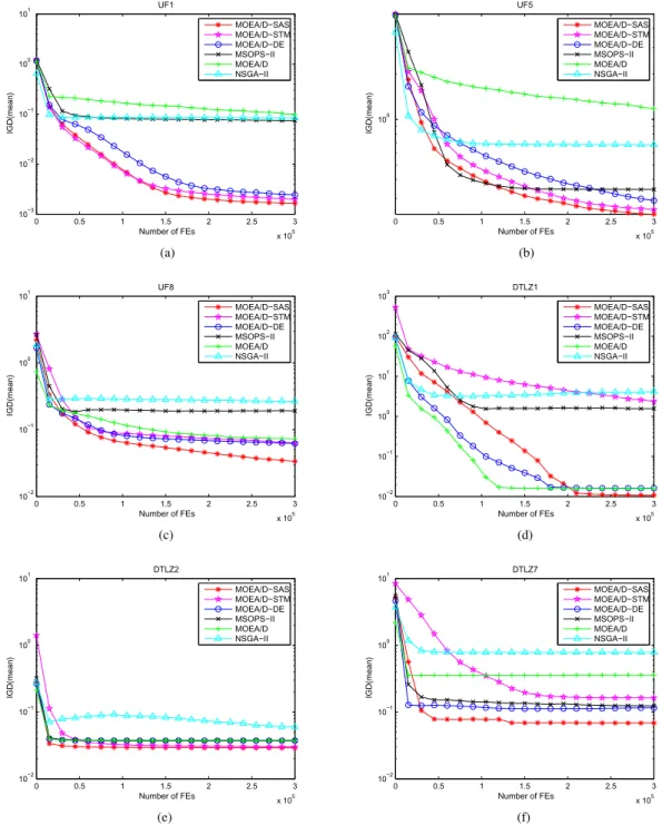
To compare the performance of algorithms during the opti-mization process, the evolution of the average IGD values, versus the number of function evaluations, for UF and DTLZ test instances are plotted in Fig.3. It can be seen clearly from these figures that MOEA/D-SAS almost always has the best performances on both convergence speed and quality of the final nondominated sets. This observation is consistent with our motivations in Section I.
TABLE IV
MEAN ANDSTANDARDDEVIATIONVALUES OFIGD, OBTAINED BY MOEA/D-SASANDMOEA/D-STMONUFANDDTLZ INSTANCES
B. Comparisons With MOEA/D-STM
MOEA/D-STM [28] is a state-of-the-art MOEA/D variant, which adopts an STM model to balance the convergence and diversity in the selection process of MOEA/D. In this section, we compare MOEA/D-SAS with it.
Table IV shows the performance of MOEA/D-SAS and MOEA/D-STM in terms of IGD. We can observe that the per-formances of MOEA/D-SAS are significantly better than that of MOEA/D-STM on 12 out of 17 test functions, although its performance is significantly worse than that of MOEA/D-STM on UF3. The two compared algorithms have very similar performances on UF2, UF4, UF6, and UF9.
Fig. 3. Convergence graphs in terms of IGD (mean) obtained by MOEA/D-SAS, MOEA/D, MOEA/D-DE, MSOPS-II, NSGA-II, and MOEA/D-STM on three UF and three DTLZ instances. Convergence plot of six algorithms on (a) UF1, (b) UF5, (c) UF8, (d) DTLZ1, (e) DTLZ2, and (f) DTLZ7.
Fig. 4 plots all the populations over 30 independent runs obtained by MOEA/D-SAS, MOEA/D-STM, and MOEA/D-DE on UF2, UF8, DTLZ1, and DTLZ7. It is very clear that MOEA/D-SAS performs best among the three algo-rithms. It is worth to note that, for the benchmark problem with a disconnected and degenerate PF, such as DTLZ7, MOEA/D-STM tends to obtain the boundary solutions in PF, as illustrated in Fig. 1 and explained in Section I, while MOEA/D-SAS is able to obtain more diverse Pareto approximate solutions.
C. Computational Efficiency of Decomposition-Based-Sorting
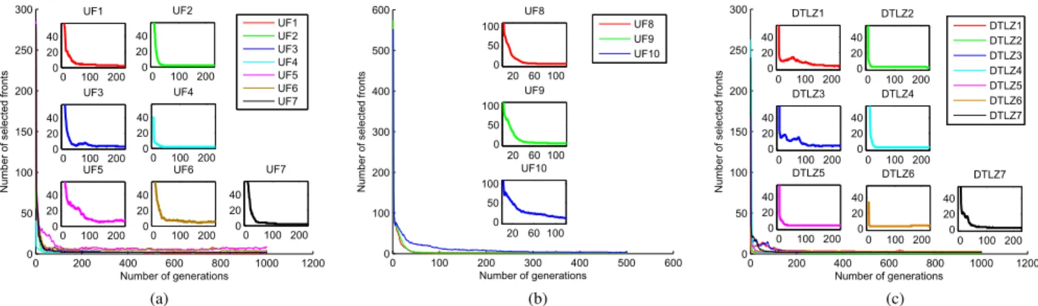
DBS conducts sorting only among the neighboring solutions for each subproblem, which effectively reduces its
computational cost. The number of selected fronts (α) at each generation adaptively determines the number of clos-est solutions to the direction vectors of subproblems L, for the next generation, and thus, plays an important role on the computational efficiency of DBS. Fig. 5 plots the evolution of α at each generations on different benchmark problems. It can be observed that the values of α decrease very quickly during the evolutionary process and level off at a very small value (α N), in all the benchmark
problems. These observations further support the motivations in Section I and analysis in Section III, that DBS is able to use local neighborhood information to reduce its computa-tional cost.
Fig. 4. Plots of all the final populations over 30 independent runs obtained by MOEA/D-SAS, MOEA/D-STM, and MOEA/D-DE on two UF instances and two DTLZ instances. The solution set obtained by (a) MOEA/D-SAS on UF2, (b) MOEA/D-STM on UF2, (c) MOEA/D-DE on UF2, (d) MOEA/D-SAS on UF8, (e) MOEA/D-STM on UF8, (f) MOEA/D-DE on UF8, (g) MOEA/D-SAS on DTLZ1, (h) MOEA/D-STM on DTLZ1, (i) MOEA/D-DE on DTLZ1, (j) MOEA/D-SAS on DTLZ7, (k) MOEA/D-STM on DTLZ7, and (l) MOEA/D-DE on DTLZ7.
D. Effects of Angle-Based-Selection
The ABS is proposed as a fine-grained diversity main-tenance scheme in SAS. In this section, the effects of it are investigated and analyzed. We compare MOEA/D-SAS with a variant of itself [named MOEA/D-SAS(a)], in which the ABS is eliminated. The comparisons between these two algorithms can be considered as a way to test the effects
of ABS. In addition, we also replace ABS with niche-counts [14], for MOEA/D-SAS. This variant of MOEA/D-SAS [named MOEA/D-SAS(n)] is also compared with the original MOEA/D-SAS.
The experimental results of comparing MOEA/D-SAS with MOEA/D-SAS(a) and MOEA/D-SAS(n) are presented in Table V. It can be observed that the performances
Fig. 5. Number of selected fronts versus the number of generations in the evolutionary process. (a) UF1-7. (b) UF8-10. (c) DTLZ107.
TABLE V
MEAN ANDSTANDARDDEVIATIONVALUES OFIGD, OBTAINED BYMOEA/D-SAS, MOEA/D-SAS(a), ANDMOEA/D-SAS(n)ONUFANDDTLZ INSTANCES
TABLE VI
PARAMETERSETTINGS INMOEA/D-SASANDNSGA-IIIFORMANY-OBJECTIVEBENCHMARKPROBLEMS
of MOEA/D-SAS are significantly better than that of MOEA/D-SAS(a) on 8 out of 17 benchmark problems. The performances between these two algorithms have no signifi-cant differences on the other nine benchmark problems. The results validate that ABS is very effective to improve the diversity of the population in most cases.
In addition, the performances of MOEA/D-SAS are signif-icantly better on six benchmark problems and worse on one problem than that of MOEA/D-SAS(n). Both algorithms have very similar performances on the rest of benchmark prob-lems. The above results are consistent with our motivations in Section I that ABS is more fine-grained than niche-counts scheme.
E. Performance of MOEA/D-SAS on Many-Objective Optimization Problems
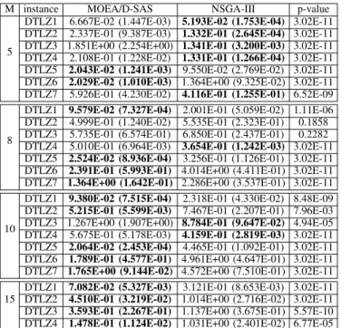
1) MOEA/D-SAS Versus NSGA-III: NSGA-III [14], which is a state-of-the-art variant of NSGA-II, has shown very good performance on MOPs. In this section, MOEA/D-SAS and NSGA-III are compared on the 5-, 8-, 10-, and 15-objective DTLZ test problems. PBI is used as the decomposition approach for MOEA/D-SAS, where the penalty parameter β is set to 3 for DTLZ3 and 10 for all other test problems. More details with regard to the parameter settings are listed in TableVI.
The performance of MOEA/D-SAS and NSGA-III, in terms of IGD values, are presented in TableVII. It can be observed
Fig. 6. Parallel coordinate plots for the nondominated solution set in the best run obtained by MOEA/D-SAS (left column) and NSGA-III (right column) on 10-objective DTLZ problems. The middle column shows the parallel coordinate plots of the reference solution sets sampled from the true PFs. (a), (d), (g), and (j) MOEA/D-SAS. (b), (e), (h), and (k) True PFs. (c), (f), (i), and (l) NSGA-III.
that MOEA/D-SAS is able to outperform NSGA-III on most test problems and MOEA/D-SAS has the increasingly better performance than NSGA-III when the number of objectives increases. It is also worth to note that DTLZ5 and DTLZ6 are the degenerated test problems, whose PFs are irregu-lar. Nevertheless, MOEA/D-SAS constantly achieves better performance than NSGA-III on these two test problems.
To show the convergence and diversity for these two compared algorithms, the parallel coordinate plots of the solu-tion sets obtained from the best run for MOEA/D-SAS and NSGA-III are shown in Fig. 6. It is clear to see that MOEA/D-SAS achieves much better diversity than NSGA-III on DTLZ1 and DTLZ2. For DTLZ5 and DTLZ6 whose PFs are degen-erate, the shapes of parallel coordinate plots obtained by
TABLE VII
MEAN ANDSTANDARDDEVIATIONVALUES OFIGD, OBTAINED BY MOEA/D-SASANDNSGA-IIIONDTLZ INSTANCES
TABLE VIII
MEAN ANDSTANDARDDEVIATIONVALUES OFIGD, OBTAINED BY MOEA/D-SASANDMOEA/D-AWAONDTLZ TESTPROBLEMS
WITHDISCONNECTED ANDDEGENERATEPFS
MOEA/D-SAS is much more similar to that of true PFs than the ones obtained by NSGA-III.
2) MOEA/D-SAS Versus MOEA/D-AWA: In the MOEA/D
with adaptive weight adjustment (MOEA/D-AWA) [33], an adaptive weight vector adjustment strategy is introduced. The weight vectors of subproblems are adjusted periodically to be redistributed adaptively for obtaining better uniformity of solu-tions. Different from MOEA/D-AWA, MOEA/D-SAS uses the fixed set of weight vectors. However, different solutions can be associated with the same subproblems; and some subprob-lems are allowed to have no associated solution. To compare the effects of MOEA/D-AWA and MOEA/D-SAS on irregular MOPs, experiments are conducted between these two algo-rithms on 5-, 8-, and 10-objective DTLZ5–7 test problems that
have disconnected or degenerate PFs, as shown in TableVIII. It can be seen that MOEA/D-SAS performs significantly better than MOEA/D-AWA on all DTLZ5-6 test problems though it performs worse than MOEA/D-AWA on DTLZ7.
VII. CONCLUSION
This paper proposed an SAS as the selection operator for MOEA/D to address MOPs. In SAS, the balance between convergence and diversity is achieved by two components, DBS and ABS. Different from other selection schemes, e.g., global STM model, DBS only conducts sorting within the local neighboring solutions, which drastically reduce the com-putational cost of SAS. Meanwhile, ABS utilizes the angle information in the objective space to maintain a fine-grained diversity. Different from many other MOEA/D variants, SAS allows one subproblem to associate with any number of solu-tions, or even no solusolu-tions, which makes it more flexible for MOPs with different shapes of PFs. SAS is integrated into MOEA/D and the algorithm, called MOEA/D-SAS, is com-pared with four classical (NSGA-II, MSOPS-II, MOEA/D, and MOEA/D-DE) and three state-of-the-art MOEAs (MOEA/D-STM, NSGA-III, and MOEA/D-AWA) on continuous MOPs or MaOPs. The experimental results show that MOEA/D-SAS outperforms other compared algorithms. In addition, the com-putational efficiency of DBS and the effects of ABS are also discussed in this paper in detail.
REFERENCES
[1] M. Asafuddoula, T. Ray, and R. A. Sarker, “A decomposition-based evolutionary algorithm for many objective optimization,” IEEE Trans.
Evol. Comput., vol. 19, no. 3, pp. 445–460, Jun. 2015.
[2] J. Bader and E. Zitzler, “Hype: An algorithm for fast hypervolume-based many-objective optimization,” Evol. Comput., vol. 19, no. 1, pp. 45–76, 2011.
[3] N. Beume, B. Naujoks, and M. Emmerich, “SMS-EMOA: Multiobjective selection based on dominated hypervolume,” Eur. J. Oper. Res., vol. 181, no. 3, pp. 1653–1669, Sep. 2007.
[4] P. A. N. Bosman and D. Thierens, “The balance between proximity and diversity in multiobjective evolutionary algorithms,” IEEE Trans. Evol.
Comput., vol. 7, no. 2, pp. 174–188, Apr. 2003.
[5] Q. Cai, M. Gong, S. Ruan, Q. Miao, and H. Du, “Network structural balance based on evolutionary multiobjective optimization: A two-step approach,” IEEE Trans. Evol. Comput., vol. 19, no. 6, pp. 903–916, Dec. 2015.
[6] X. Cai, Y. Li, Z. Fan, and Q. Zhang, “An external archive guided multiobjective evolutionary algorithm based on decomposition for combinatorial optimization,” IEEE Trans. Evol. Comput., vol. 19, no. 4, pp. 508–523, Aug. 2015.
[7] R. Cheng, Y. Jin, K. Narukawa, and B. Sendhoff, “A multiobjective evolutionary algorithm using Gaussian process-based inverse modeling,”
IEEE Trans. Evol. Comput., vol. 19, no. 6, pp. 838–856, Dec. 2015.
[8] C. A. C. Coello and N. C. Cortés, “Solving multiobjective optimization problems using an artificial immune system,” Genet. Program. Evol.
Mach., vol. 6, no. 2, pp. 163–190, 2005.
[9] C. A. C. Coello, “Evolutionary multi-objective optimization: A historical view of the field,” IEEE Comput. Intell. Mag., vol. 1, no. 1, pp. 28–36, Feb. 2006.
[10] C. A. C. Coello, G. B. Lamont, and D. A. Van Veldhuizen, Evolutionary
Algorithms for Solving Multi-Objective Problems, 2nd ed. New York,
NY, USA: Springer, Sep. 2007.
[11] I. Das and J. E. Dennis, “Normal-boundary intersection: A new method for generating the Pareto surface in nonlinear multicriteria optimization problems,” SIAM J. Optim., vol. 8, no. 3, pp. 631–657, 1998. [12] K. Deb, Multi-Objective Optimization Using Evolutionary Algorithms.
[13] K. Deb and M. Goyal, “A combined genetic adaptive search (GeneAS) for engineering design,” Comput. Sci. Informat., vol. 26, no. 4, pp. 30–45, 1996.
[14] K. Deb and H. Jain, “An evolutionary many-objective optimization algorithm using reference-point-based nondominated sorting approach, part I: Solving problems with box constraints,” IEEE Trans. Evol.
Comput., vol. 18, no. 4, pp. 577–601, Aug. 2014.
[15] K. Deb, A. Pratap, S. Agarwal, and T. Meyarivan, “A fast and elitist multiobjective genetic algorithm: NSGA-II,” IEEE Trans. Evol. Comput., vol. 6, no. 2, pp. 182–197, Apr. 2002.
[16] K. Deb, L. Thiele, M. Laumanns, and E. Zitzler, “Scalable test prob-lems for evolutionary multiobjective optimization,” Evolutionary
Multiobjective Optimization. London, U.K.: Springer, 2005, pp. 105–145.
[17] J. J. Durillo, A. J. Nebro, F. Luna, and E. Alba, “On the effect of the steady-state selection scheme in multi-objective genetic algorithms,” in
Proc. 5th Int. Conf. Evol. Multi-Criterion Optim. (EMO), vol. 5467.
Nantes, France, Apr. 2009, pp. 183–197.
[18] C. M. Fonseca and P. J. Fleming, “An overview of evolutionary algo-rithms in multiobjective optimization,” Evol. Comput., vol. 3, no. 1, pp. 1–16, 1995.
[19] S. B. Gee, K. C. Tan, V. A. Shim, and N. R. Pal, “Online diversity assessment in evolutionary multiobjective optimization: A geometrical perspective,” IEEE Trans. Evol. Comput., vol. 19, no. 4, pp. 542–559, Aug. 2015.
[20] E. J. Hughes, “MSOPS-II: A general-purpose many-objective optimiser,” in Proc. IEEE Congr. Evol. Comput. (CEC), Singapore, Sep. 2007, pp. 3944–3951.
[21] E. J. Hughes, “Multiple single objective Pareto sampling,” in Proc.
Congr. Evol. Comput. (CEC), vol. 4. Canberra, ACT, Australia,
Dec. 2003, pp. 2678–2684.
[22] H. Ishibuchi, H. Masuda, and Y. Nojima, “Pareto fronts of many-objective degenerate test problems,” IEEE Trans. Evol. Comput., to be published.
[23] H. Ishibuchi, Y. Sakane, N. Tsukamoto, and Y. Nojima, “Adaptation of scalarizing functions in MOEA/D: An adaptive scalarizing function-based multiobjective evolutionary algorithm,” in Proc. 5th Int. Conf.
Evol. Multi Criterion Optim. (EMO), vol. 5467. Nantes, France,
Apr. 2009, pp. 438–452.
[24] B. Li, K. Tang, J. Li, and X. Yao, “Stochastic ranking algorithm for many-objective optimization based on multiple indicators,” IEEE Trans.
Evol. Comput., Mar. 2016, doi: 10.1109/TEVC.2016.2549267. .
[25] H. Li and Q. Zhang, “Multiobjective optimization problems with compli-cated Pareto sets, MOEA/D and NSGA-II,” IEEE Trans. Evol. Comput., vol. 13, no. 2, pp. 284–302, Apr. 2009.
[26] K. Li, K. Deb, Q. Zhang, and S. Kwong, “An evolutionary many-objective optimization algorithm based on dominance and decompo-sition,” IEEE Trans. Evol. Comput., vol. 19, no. 5, pp. 694–716, Oct. 2015.
[27] K. Li, S. Kwong, Q. Zhang, and K. Deb, “Inter-relationship based selection for decomposition multiobjective optimization,” IEEE Trans.
Cybern., vol. 45, no. 10, pp. 2076–2088, Oct. 2015.
[28] K. Li, Q. Zhang, S. Kwong, M. Li, and R. Wang, “Stable matching-based selection in evolutionary multiobjective optimization,” IEEE Trans. Evol.
Comput., vol. 18, no. 6, pp. 909–923, Dec. 2014.
[29] H.-L. Liu, F. Gu, and Q. Zhang, “Decomposition of a multiobjective optimization problem into a number of simple multiobjective sub-problems,” IEEE Trans. Evol. Comput., vol. 18, no. 3, pp. 450–455, Jun. 2014.
[30] K. Miettinen, Nonlinear Multiobjective Optimization. Boston, MA, USA: Kluwer Academic, 1999.
[31] T. Murata, H. Ishibuchi, and M. Gen, “Specification of genetic search directions in cellular multi-objective genetic algorithms,” in Proc. 1st
Int. Conf. Evol. Multi-Criterion Optim., Zürich, Switzerland, 2001,
pp. 82–95.
[32] K. Price, R. M. Storn, and J. A. Lampinen, Differential Evolution:
A Practical Approach to Global Optimization (Natural Computing
Series). Heidelberg, Germany: Springer, 2005.
[33] Y. Qi et al., “MOEA/D with adaptive weight adjustment,” Evol. Comput., vol. 22, no. 2, pp. 231–264, 2014.
[34] A. B. Ruiz, R. Saborido, and M. Luque, “A preference-based evolutionary algorithm for multiobjective optimization: The weighting achievement scalarizing function genetic algorithm,” J. Glob. Optim., vol. 62, no. 1, pp. 101–129, 2015.
[35] J. D. Schaffer and J. J. Grefenstette, “Multi-objective learning via genetic algorithms,” in Proc. 9th Int. Joint Conf. Artif. Intell. (IJCAI), Los Angeles, CA, USA, 1985, pp. 593–595.
[36] X.-N. Shen and X. Yao, “Mathematical modeling and multi-objective evolutionary algorithms applied to dynamic flexible job shop scheduling problems,” Inf. Sci., vol. 298, pp. 198–224, Mar. 2015.
[37] K. C. Tan, E. F. Khor, and T. H. Lee, Multiobjective Evolutionary
Algorithms and Applications (Advanced Information and Knowledge
Processing). London, U.K.: Springer, 2005.
[38] J. Wang et al., “Multiobjective vehicle routing problems with simulta-neous delivery and pickup and time windows: Formulation, instances, and algorithms,” IEEE Trans. Cybern., vol. 46, no. 3, pp. 582–594, Mar. 2016.
[39] R. Wang, Q. Zhang, and T. Zhang, “Decomposition based algorithms using Pareto adaptive scalarizing methods,” IEEE Trans. Evol. Comput., to be published.
[40] Q. Zhang and H. Li, “MOEA/D: A multiobjective evolutionary algorithm based on decomposition,” IEEE Trans. Evol. Comput., vol. 11, no. 6, pp. 712–731, Dec. 2007.
[41] Q. Zhang et al., “Multiobjective optimization test instances for the CEC 2009 special session and competition,” School Comput. Sci. Elect. Eng., Univ. Essex, Colchester, U.K. and Nanyang Technol. Univ., Singapore, and Nanyang Technol. Univ., Singapore, Tech. Rep. CES-487, 2008. [42] X. Zhang, Y. Tian, R. Cheng, and Y. Jin, “An efficient approach to
non-dominated sorting for evolutionary multiobjective optimization,” IEEE
Trans. Evol. Comput., vol. 19, no. 2, pp. 201–213, Apr. 2015.
[43] E. Zitzler and S. Künzli, “Indicator-based selection in multiobjec-tive search,” in Parallel Problem Solving From Nature—PPSN VIII (LNCS 3242), X. Yao et al., Eds. Heidelberg, Germany: Springer-Verlag, Sep. 2004, pp. 832–842.
[44] E. Zitzler, M. Laumanns, and L. Thiele, “SPEA2: Improving the strength Pareto evolutionary algorithm for multiobjective opti-mization,” in Evolutionary Methods for Design, Optimization and
Control With Applications to Industrial Problems—EUROGEN 2001,
K. C. Giannakoglou, D. Tsahalis, J. Periaux, P. Papailou, and T. Fogarty, Eds. Athens, Greece: CIMNE, 2002, pp. 95–100. [45] E. Zitzler, L. Thiele, M. Laumanns, C. M. Fonseca, and
V. G. da Fonseca, “Performance assessment of multiobjective optimizers: An analysis and review,” IEEE Trans. Evol. Comput., vol. 7, no. 2, pp. 117–132, Apr. 2003.