University of Toronto
Department of Economics
December 18, 2007
By Chun Liu and John M Maheu
Are there Structural Breaks in Realized Volatility?
Are there Structural Breaks in Realized Volatility?
Chun Liu
School of Economics and Management
Tsinghua University
John M. Maheu
∗Dept. of Economics
University of Toronto
November 2007
AbstractConstructed from high-frequency data, realized volatility (RV) provides an effi-cient estimate of the unobserved volatility of financial markets. This paper uses a Bayesian approach to investigate the evidence for structural breaks in reduced form time-series models of RV. We focus on the popular heterogeneous autoregressive (HAR) models of the logarithm of realized volatility. Using Monte Carlo simula-tions we demonstrate that our estimation approach is effective in identifying and dating structural breaks. Applied to daily S&P 500 data from 1993-2004, we find strong evidence of a structural break in early 1997. The main effect of the break is a reduction in the variance of log-volatility. The evidence of a break is robust to different models including a GARCH specification for the conditional variance of log(RV).
key words: realized volatility, change point, marginal likelihood, Gibbs sampling, GARCH
JEL: C22, C11, G10
1
Introduction
The econometric modeling of volatility is an important issue in empirical finance. Instabil-ity of the volatilInstabil-ity process has important implications for decisions in risk management,
∗We thank Gordon Anderson, Gael Martin, Alex Maynard, Angelo Melino, and Tom McCurdy for
helpful comments. Maheu is grateful for funding from SSHRC. Corresponding author: J. Maheu, 100 St. George St., University of Toronto, Dept. of Economics, Toronto, Ontario M5S 3G3, Canada, 905-828-5375, [email protected]
portfolio choice and derivative pricing. Many papers have studied the effect of neglected parameter changes on the level and persistence of volatility1. Another strand of the
litera-ture has focused on testing for structural breaks2, or directly modeling parameter change.3
A common feature of this research is the use of stock returns to infer structural changes in the latent volatility process.
Recently, a new observable measure of volatility, called realized volatility (RV) has been proposed. Realized volatility uses high-frequency data information and has been shown to be an accurate estimate of ex post volatility. RV is constructed from the sum of intraday squared returns, and converges to quadratic variation which is the sum of integrated volatility plus a jump component for a broad class of continuous time models. This is an essentially nonparametric estimate of ex post volatility. Barndorff-Nielsen and Shephard (2004) show how the continuous component can be separated from the jump component of volatility. Empirical and theoretical features of RV are discussed by An-dersen and Bollerslev (1998), AnAn-dersen, Bollerslev, Diebold and Labys (2001), AnAn-dersen, Bollerslev, Diebold and Ebens (2001), Barndorff-Nielsen and Shephard (2002a,2002b), and Meddahi (2002). The purpose of this paper is to investigate the evidence for struc-tural breaks within the context of popular time-series models of RV. The use of realized volatility, in contrast to daily returns, will provide us with more power to detect structural changes.
An important feature of the time-series of RV is the strong serial dependence.4 Corsi
(2004) shows that the heterogeneous autoregressive (HAR) model can capture the strong persistence in the data with a parsimonious linear structure. This is not a true long-memory model but it does provide a good approximation to the dynamics of long-long-memory. These features make this specification popular and easy to estimate. HAR type parame-terizations appear in recent research including Andersen, Bollerslev and Diebold (2006), Andersen, Bollerslev and Huang (2007), Bollerslev et al. (2007), Corsi et al. (2005), Forsberg and Ghysels (2006), and Maheu and McCurdy (2006).
This paper provides a Bayesian analysis of structural breaks in daily S&P 500 realized
1Examples include Chu (1995), Hillebrand (2005), Hwang and Pereira (2004), Lamoureux and
Las-trapes (1990), Mikosch and Starica (2004), and Starica and Granger (2005) among others.
2Andreou and Ghysels (2002), Pastor and Stambaugh (2001), Rapach and Strauss (2006), Ray and
Tsay (2002), and Smith (2006).
3For instance, Engle and Rangel (2005).
4Different models that account for this include: autoregressive fractional integrated moving average
(ARFIMA) models by Andersen, Bollerslev, Diebold and Labys (2003), Giot and Laurent (2004), and Martins, van Dijk and de Pooter (2004); Markov switching in Maheu and McCurdy (2002); unobserved component models, Barndorff-Nielsen and Shephard (2002a) and Koopman, Jungbacker and Hol (2005); the mixed data sampling approach of Ghysels et al. (2003); and the heterogeneous autoregressive model of Corsi (2004).
volatility. We focus on a logarithmic HAR specification similar to Andersen et al. (2006), and an extension to include GARCH effects. We test for multiple structural breaks using the change-point (or structural break) model of Chib (1998) which is estimated with efficient Markov chain Monte Carlo sampling methods. We investigate specifications which allow for all parameters, as well as only a subset of parameters, to change due to a structural break. This allows us to isolate the impact of a break on individual model parameters and to use all data in the estimation of parameters not affected by breaks. Each model is estimated conditional on 0,1,2, ..., kmaxbreaks occurring. For each of these
we calculate the marginal likelihood, and the evidence for the number of breaks can be compared using Bayes factors.5
A first step is to investigate the power of the Chib change-point model to detect the correct number of structural breaks. The simulations, based on empirically realistic models, show the method to perform well in estimating the true number of breaks when there are 1 or more breaks, as well as when there are no breaks. The larger the number of parameters that are affected by a break, the more likely the structural breaks are correctly identified. In addition, it is relatively more difficult to identify several structural breaks, particularly when only one model parameter changes.
We find the marginal likelihood has an advantage over traditional model comparison criteria, such as sum of squared errors, in identifying the true number of structural breaks. For example, in-sample loss functions of one period ahead forecasts of RV are less sen-sitive to structural breaks. In fact, the R2 from commonly used Mincer and Zarnowitz
(1969) forecast regressions strongly favor models with more change-points than there are. Forecasting loss functions are less powerful in detecting breaks and can be a misleading indicator of structural breaks.
The empirical results for S&P 500 provide strong evidence of a structural break in the logarithm of RV (log-RV) during February 1997 based on data from 1993-2004. The effect of the structural break is mainly confined to the variance with weaker evidence that the regression parameters are effected. The structural break results in a smaller variance after 1997. The conclusions are robust to the inclusion/exclusion of jumps, and asymmetric terms in the model.
Concurrent work by Andersen et al. (2006), Andersen et al. (2007), Corsi et al. (2005), and Bollerslev et al. (2007) using a similar model for S&P 500 volatility ignore the possibility of structural breaks. We demonstrate that accounting for the structural break improves out-of-sample density forecasts of log-volatility dramatically after the
5Related applications of Bayesian change-point analysis include Kim et al. (2005), Martin (2000),
break point. Corsi et al. (2005), Andersen et al. (2007) and Bollerslev et al. (2007) use a HAR model for volatility and allow for GARCH effects in the conditional variance. To investigate if our finding of a break is spurious due to neglected conditional variance dynamics, we consider breaks in a HAR-GARCH model for log-RV. Again the evidence is strong for a break in the long-run variance from the GARCH model and the estimated break point is identical to that of the homoskedastic model. Moreover, ignoring this break results in persistence estimates in the GARCH model that are too high. In summary, we find a permanent reduction in the variance of log-RV in February 1997 for all of our specifications. Failure to model this break results in biased parameter estimates and poor density forecasts.
The structure of this paper is as follows. In Section 2 we review the construction of RV and the jump component, and the empirical model for daily log-RV. The change-point model and Bayesian estimation are detailed in Section 3. Section 4 presents simulation results on the ability of the change-point model to detect breaks, date change points and other features. Section 5 is the application to S&P 500 volatility while Section 6 concludes. An appendix provides details on the estimation of the marginal likelihood and the HAR-GARCH model.
2
Realized Volatility
2.1
Estimation
We assume that the price process belongs to the class of special semimartingales, which is a very broad class of processes including Ito and jump processes. In this environment Andersen, Bollerslev, Diebold and Labys (2001) show that the quadratic variation of the process, which is defined as integrated volatility plus the jump component, provides a natural measure of ex post volatility. RV is constructed from the sum of intraday squared returns and is a consistent estimate of quadratic variation as the intraday sampling fre-quency goes to infinity. In contrast to traditional measures of volatility, such as daily squared returns, realized volatility is more efficient. Andersen and Bollerslev (1998), Barndorff-Nielsen and Shephard (2002b) and Meddahi (2002) discuss the precision of RV. Market microstructure dynamics contaminate the price process with noise. The noise can be time dependent and may be correlated with the efficient price (Hansen and Lunde (2006)). RV can be a biased and inconsistent estimator. For instance see Bandi and Russell (2006), Hansen and Lunde (2006), Oomen (2005) and Zhang et al. (2005) for more details on the effects of market microstructure noise on volatility estimation. To
reduce the effect of market microstructure noise, we employ a kernel-based estimator that utilizes autocovariances of intraday returns. Specifically, we follow Hansen and Lunde (2006) to provide a bias correction to realized volatility as follows,6
RVt = M X i=1 r2 t,i+ 2 q X h=1 µ 1− h q+ 1 ¶MX−h i=1 rt,irt,i+h (1)
where rt,i is the ith logarithmic return during day t, M is the number of returns in each day, and q = 1 in our calculations. This estimator is guaranteed to be non-negative and is almost identical to the subsample-based estimator of Zhang et al. (2005).
Barndorff-Nielsen and Shephard (2004) show how the continuous component can be separated from the jump component of volatility. They define realized bipower variation as, RBPt=µ−12 MX−1 i=1 |rt,i||rt,i+1|, (2) where µ1 = p
2/π. Asymptotically as M → ∞, realized bipower variation converges to integrated volatility. The difference between RVt and RBPt is an estimate of the daily jump component. In our paper, we follow Andersen et al. (2006) and estimate jumps by,
Jt=
(
log (RVt−RBPt+ 1) when RVt−RBPt>0
0 Otherwise (3)
where we add 1 to ensure thatJt≥0.
2.2
Models
Consider the heterogeneous autoregressive model (HAR) of realized volatility proposed by Corsi (2004). Corsi shows that this model can capture many of the features of volatility including long memory. Empirically the distribution of log(RVt) is approximately bell shaped7, so we consider a logarithmic version of the HAR similar to that implemented by
Andersen et al. (2006) and defined as
vt=β0+β1vt−1+β2vt−5,t−1+β3vt−22,t−1+²t, ²t∼NID(0, σ2). (4)
6The adjustedRV
t from Hansen and Lunde produced several days with a negative estimate forRVt.
We follow their suggestion and use Bartlett weights to ensure thatRVt is positive. The estimator is no
longer unbiased, but may have a smaller MSE.
7See Andersen, Bollerslev, Diebold and Labys (2001), Andersen, Bollerslev, Diebold and Ebens (2001),
wherevt= log(RVt) and vt−5,t−1 =
log (RVt−1) + log (RVt−2) +· · ·+ log (RVt−5)
5 (5)
vt−22,t−1 =
log (RVt−1) + log (RVt−2) +· · ·+ log (RVt−22)
22 (6)
This model postulates three factors that affect volatility: daily log-volatilityvt−1, weekly
log-volatilityvt−5,t−1 and monthly log-volatility vt−22,t−1.
Andersen et al. (2006), Huang and Tauchen (2005), and Tauchen and Zhou (2005) conclude that jumps are an important component of realized volatility. Therefore, we consider a model with a jump component as well as asymmetric terms motivated by the models in Bollerslev et al. (2007),
vt =β0+β1vt−1+β2vt−5,t−1+β3vt−22,t−1+βJJt−1+βA1 |rt−1| √ RVt−1 +βA2 |rt−1| √ RVt−1 I(rt−1 <0)+²t (7) where rt is the daily return, I(rt−1 <0) is an indicator function, which equals 1 when
rt−1 < 0 and equals 0 otherwise. Jt−1 is the jump component defined above. The last
two terms allow for asymmetric effects from positive and negative returns similar to the EGARCH model of Nelson (1991).
To simplify the notation, we note that the model can be cast into a standard regression form yt =Xtβ+²t whereyt=vt, β= [β0 β1 β2 β3 βJ βA1 βA2] 0 and Xt = · 1vt−1 vt−5,t−1 vt−22,t−1 Jt−1 |rt−1| √ RVt−1 |rt−1| √ RVt−1 I(rt−1 <0) ¸ . In the following denote Yt={v1, v2, . . . , vt}, and It={y1, X1, ..., yt, Xt}.
3
Change-point Model
We consider the change-point (or structural break) model proposed by Chib (1998). This uses a hidden Markov model with a restricted transition matrix to model change-points. A test for the number of breaks is then a test of the dimension of the hidden Markov chain. As Chib shows there are efficient posterior simulation methods available for this type of model. Model parameters and change points are jointly estimated conditional on a fixed number of change points. Bayes factors can be used to compare the evidence for
the number of breaks.
In the following we review a Gibbs sampling approach for the unrestricted model in which all parameters are subject to change after a break. This is followed by a discussion of the restricted model in which some parameters are restricted to be constant across breaks. This latter specification allows us to isolate which features of the model are most likely affected by a structural break.
Assume there are m − 1, m ∈ {1,2, ...} change points at unknown times Ωm =
{τ1, τ2, . . . , τm−1}. Separated by those change points, we have m different regimes. The
density of observation yt, t = 1,2,· · · , T, depends on the parameter θk = {βk, σ2
k}, k = 1, ..., m, whose value changes at the change points Ωm and remains constant oth-erwise θt= θ1 if t < τ1 θ2 if τ1 ≤t < τ2 ... ... ... θm−1 if τm−2 ≤t < τm−1 θm if τm−1 ≤t. (8)
Denote the state of the system at each time by S = {s1, s2, . . . , sT} where st = k indicates that the observationytis from regimek and follows the conditional distribution f(yt|It−1, θk). The one-step ahead transition probability matrix forst is assumed to be
P = p11 p12 0 · · · 0 0 p22 p23 · · · 0 ... ... ... ... ... ... ... 0 pm−1,m−1 pm−1,m 0 0 · · · 0 1 (9)
where pij = Pr (st=j|st−1 =i) withj =i or i+ 1, and this is the probability of moving
from regime i at time t−1 to regime j at time t. The transition matrix ensures that given st = k at time t, the next period t+ 1, st+1 remains in the same state or jumps
to the next state. For instance, given st = k, we have st+1 = k or st+1 = k + 1 and
pk,k +pk,k+1 = 1. Once we move to the last regime m, we stay there for ever, that is
3.1
Bayesian Estimation
To conduct model estimation, we use Bayesian methods. We specify independent condi-tionally conjugate priors for the parameters. They are
βk ∼N(d0, B0), σk2 ∼IG µ v0 2, l0 2 ¶ , pii∼Beta(a0, b0) (10)
for k = 1, ..., m, and i = 1, ..., m−1, and where IG(·,·) denotes the inverse Gamma distribution. For a detailed discussion of prior selection in the context of change-point models see Koop and Potter (2004).
3.1.1 Gibbs Sampling
Although the posterior for the model is not a well known distribution, we can obtain samples from the posterior based on a Gibbs sampling scheme. Good introductions to Gibbs sampling and Markov chain Monte Carlo methods can be found in Chib (2001), and Geweke (2005).
We divide the parameters into 3 blocks: parameters of the HAR model Θ ={θ1, ..., θm}, the state of the systemS and the transition matrix P. We augment the parameter space to include the states so that we sample from the full posteriorp(Θ, S, P|IT). After choos-ing a startchoos-ing value, Θ(0), and P(0), Gibbs sampling requires we iterate sampling from the
following conditional densities
• S|P,Θ, IT
• P|S,Θ, IT
• Θ|S, P, IT
After dropping a set of burn-in samples to ensure convergence, we collect the remaining draws {P(h),Θ(h), S(h)}R
h=1 to approximate the posterior distribution. To ensure these
draws have converged to the stationary distribution, we investigate running the chain from different starting values and compute convergence diagnostics such as Geweke (1992).8
For a sufficiently large posterior sample, any function of interest can be consistently estimated. For example,
[ g(θk) = 1 R R X h=1 g(θ(kh)) (11)
8All results in this paper are robust to different starting values. For instance, we consider many
is a simulation consistent estimate ofE[g(θk)|IT], the posterior mean ofg(θk). Below we provide more details on each step of the Gibbs sampling.
Step 1: Simulation of S|P,Θ, IT. Chib (1996) shows that a joint draw of all states can be achieved using
p(S|Θ, P, IT) =p(sT|Θ, P, IT) TY−1
t=1
p(st|st+1,Θ, P, It) (12)
in which we sample sequentially from each density on the right hand side of (12) beginning withp(sT|Θ, P, IT), and then p(st|st+1,Θ, P, It)t=T−1, ...,1. At each step we condition on the previously drawn statest+1, until we obtain a full drawS. The individual densities
in (12) are obtained based on the following three steps. (a) Initialization: At t= 1, set p(s1 = 1|Θ, P, I1) = 1.
(b) Compute the Hamilton (1989) filter, p(st=k|Θ, P, It). This involves a prediction and an update step in which we iterate on the following from t= 2, ..., T,
p(st=k|Θ, P, It−1) = k X l=k−1 p(st−1 =l|Θ, P, It−1)plk, k= 1, ..., m, (13) p(st=k|Θ, P, It) = Ppm(st=k|Θ, P, It−1)f(yt|Θ, It−1, st =k) l=1p(st=l|Θ, P, It−1)f(yt|Θ, It−1, st=l) , k= 1, ..., m. The last equation is obtained from Bayes’ rule. Note that in (13) the summation is only from k−1 to k, due to the restricted nature of the transition matrix, and f(yt|Θ, It−1, st=k)∼N(Xtβk, σk2).
(c) Finally, Chib (1996) has shown that the individual densities in (12) are,
p(st|st+1,Θ, P, It)∝p(st|Θ, P, It)p(st+1|st, P). (14)
Thus, given sT =m, we can drawst backwards over t=T −1, T −2, . . . ,2 as
st|It, st+1,Θ, P = ( st+1 with probability ct st+1−1 with probability 1−ct where ct= p(st=k|Θ, P, It)p(st+1 =k|st=k, P) Pk l=k−1p(st=l|Θ, P, It)p(st+1 =k|st=l, P) .
Finally, note that P(s1 = 1|I1, s2,Θ, P) = 1.
Step 2: Simulation of P|S,Θ, IT. The conditional posterior for each component of P is
pii|S ∼Beta(a0+nii, b0+ 1) (15)
wherenii is the number of one-step transitions from state i to statei in the sequence S.
Step 3: Simulation of Θ|S, P, IT. The conditional posterior density ofθkonly depends on the data in regime k. Therefore, let Ybk = {yt :st=k} and Xbk = {Xt:st=k} and use standard Gibbs sampling methods for the linear model,
βk|Ybk,Xbk, σk2 ∼N(Mk, Vk) (16) where Mk =Vk(σk−2Xbk0Ybk+B0−1d0), Vk= (σk2Xbk0Xbk+B0−1)−1, and σ2 k|Ybk,Xbk, βk ∼IG µ vk 2 , lk 2 ¶ (17) wherevk=Tk+v0,lk= (Ybk−Xbkβk)0(Ybk−Xbkβk)+l0, andTkis the number of observations in regime k.
3.1.2 Only Breaks in Conditional Mean Parameters
Suppose we have a subset of regression parametersη with n elements that are subject to breaks denoted by ηk, k= 1, ..., m, while the remainderδ and the variance σ2 are not. If
we partition the regression parameter asβk = [η
0
kδ
0
]0 and reorderXt = [Ut Vt] to conform to this we carry out sampling as follows.
• To sample fromηk|δ, σ2, S, IT, for each regimek = 1,· · · , m, we use the observations
only in regime k and let ykb = {yt−Vtδ :st=k} and Xkb = {Ut :st=k} and use standard Gibbs sampling methods as in step 3.
• To sample from δ|η1, ..., ηk, σ2, S, IT, we use the model ybt = Vtδ +²t, where ybt = yt−
Pm
k=1UtηkI(st=k) where I(·) is the indicator function. Once again standard methods can be used to sample δ.
• Forσ2|η
1, ..., ηk, δ, S, IT, we sample the variance from the modelyt =
Pm
k=1UtηkI(st= k) +Vtδ+²twith ²t∼NID(0, σ2) which is a draw from the inverse gamma density.
3.1.3 Only Breaks in the Variance
Suppose only the variance changes between regimes, andβ is constant.
• Draw of σ2
k|β, S, IT, k = 1, ..., m, only uses data in each regime, this is standard as in step 3 above.
• β|σ2
1, ..., σ2k, S, IT. Due to the heteroskedasticity, we construct new data as byt = yt/σk,andXb =X/σk in each regime. Then we have the standard linear model with an error variance of 1.
Finally, note that we can consider breaks in the variance with only partial breaks in β by combining the methods in the last two subsections.
3.2
Bayes Factors
Let A denote a model parameterization in which some or all parameters are subject to breaks and conditional on k breaks occurring. Then the marginal likelihood (ML) is defined as
p(YT|A) =
Z
p(YT|A,Θ, P)p(Θ, P|A)dΘdP
which is a measure of the success the model has in accounting for the data after the parameter uncertainty has been integrated out over the prior. The term p(Θ, P|A) is the prior and p(YT|A,Θ, P) is the likelihood function and calculated as
logp(YT|A,Θ, P) = T X t=1 logf(yt|It−1,Θ, P) (18) where f(yt|It−1,Θ, P) = m X k=1 f(yt|It−1,Θ, st =k)p(st=k|Θ, P, It−1). (19)
The last term in the right hand side of Equation (19) is computed from Equation (13). For this model we can estimate the marginal likelihood following Chib (1995), the details of which are reported in the Appendix.
Once we calculate the marginal likelihood for different specifications we can compare them using Bayes factors. Note that we can compare models across the number of breaks, as well as the type of breaks (restricted versus unrestricted). Bayes factors can be used to compare any model configuration. The relative evidence for model A versus B is BFAB =p(YT|A)/p(YT|B). Kass and Raftery (1995) suggest interpreting the evidence for Aas: not worth more than a bare mention for 1≤BFAB <3; positive for 3≤BFAB <20;
strong for 20≤BFAB <150; and very strong for BFAB ≥150. Equivalently, based on a log scale, log(BFAB)>0 is evidence in favor ofA versus B.
4
Monte Carlo Simulation
In this section we use Monte Carlo simulations to investigate the ability of the change-point model to detect change-change-points, and date the time of a change-change-point. We also consider the effect of different sample sizes, and the in-sample forecasting performance. As mentioned above, a key ingredient of the analysis is the marginal likelihood which we estimate following Chib (1995). We have also calculated the marginal likelihood following Gelfand and Dey (1994) but do not report it to save space. We found a very close correspondence between the two estimates and identical conclusions from Bayes factors.
4.1
Setting
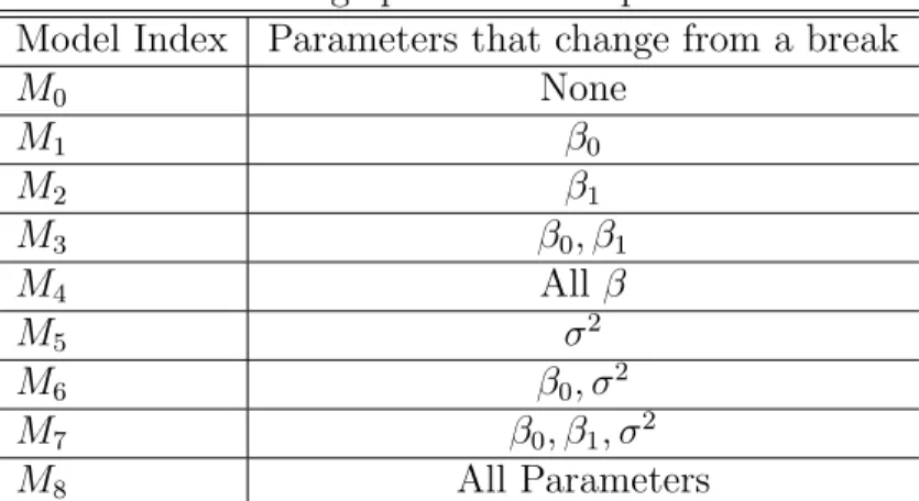
We consider the HAR model based on equation (4), in which change points affect one or more model parameters. Table 1 lists all the specifications used in the simulations and the empirical application. Specifically, M0 is the simple HAR model without any structural
change, M1 −M7 are models in which different parameters change and M8 is the model
in which all parameters change from a structural break.
For each model, we generateT = 1000 observations, which is much less than the actual data in our empirical application. Thus, we test the robustness of the method under more challenging conditions. The true models we consider include cases of no change point, 1 and 2 change points. When there is 1 change point, the position of this change point follows a uniform distribution U(0.25×T,0.75×T). When there are 2 change points, the first one follows U(0.2×T,0.4×T) and the second followsU(0.6×T,0.8×T). This setting allows us to account for the randomness of the change points as well as ensuring sufficient observations in each regime to conduct estimation.
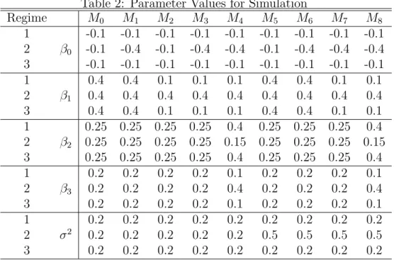
To make our simulation empirically realistic, we select parameter values of the HAR model which are close to those reported in Andersen et al. (2006). They are listed in Table 2. For example, in M0 there are no structural breaks, all parameters are constant
across regimes, while for M1 only β0 changes. If there is 1 break, β0 changes from −0.1
to−0.4. If there are 2 breaks, it changes from −0.1 to −0.4 and finally to−0.1.
The priors are βk ∼ N(0,100I), σk2 ∼ IG(0.001,0.001), k = 1, ..., m, and pii ∼ Beta(20,0.1), i = 1, ..., m−1. In this setting, βk and σ2
k are very uninformative, while the prior for pii favors infrequent structural breaks. Specifically, it means we assume the expected duration of each regime is about 201 before we see the data. However, if
there are outliers in the time series, a single point may be identified as a separate regime. To rule this out and allow for only infrequent breaks, we impose the assumption that each regime lasts at least 66 days, which is roughly 3 months in actual trading time. In practice, when we simulate a draw ofS which has a regime shorter than 66, we discard it and resample until each regime is 66 or more in length. Our results are robust to different duration restrictions which we discuss in more detail for the empirical application in Section 5. A similar strategy is followed by Kim et al. (2005) using financial data. The first 5000 samples from the posterior simulator are discarded and the next 15000 are used for posterior inference.
4.2
Identifying the Number of Change Points
In the following, the model specificationMiis assumed known but the number of structural breaks and model parameters are not known. For each draw from the data generating process (DGP), we estimate the change-point model assuming 0,1,2, and 3 structural breaks. We rank the evidence for the number of break points according to the largest marginal likelihood. The best change point specification has the largest marginal likeli-hood, while the second best has the next largest, etc. We draw a new sample of data from the DGP and repeat this until 100 repetitions are completed. Then we report the frequency over repetitions in which each specification is best according to the marginal likelihood.
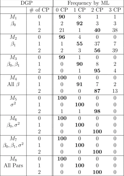
Table 3 lists the results for each of the different specifications. For convenience, bold entries in these cells should be 100 if classification is perfect. For example, the first entry (row) for M1 says that for a DGP with no change points, out of 100 repetitions 90 are
correctly identified as no change point, while 10 (8+1+1) are identified incorrectly as change points. The next entry in the table repeats this for a DGP with 1 change point. Here, 92 times 1 change point is correctly identified.
Overall the Chib model works very well. When there is no change point, this is correctly selected most of the time. Looking at the cases when data are generated from the model with no change point (first row in each panel), they are 90/100 forM1, 96/100
for M2, 99/100 for M3 and 100/100 for M4 −M8. Except for a few cases, this method
will correctly rule out structural breaks when the underlying process is actually stable. On the other hand, when the process contains change points, the Chib model correctly identifies the existence of the change points in most cases. For example, the probability of correctly identifying instability of the process is 0.98 ((92+3+3)/100) forM1 and 1 change
point, and is 0.79 for 2 change points. Furthermore, the correct number of change points are found most of the time. Looking at the numbers in bold, many of them are close
to 100. However, the relatively low numbers associated with M1 and M2 show that the
method is not as powerful when there are changes only in the interceptβ0 or only in β1.
Therefore, for this DGP it is easier to identify structural breaks when more parameters undergo a change. For example, compareM1, andM2, with the better performance ofM4
in which all β change from a break. Similarly, we see better results when the variance is subject to structural breaks. The best results of the table correspond to modelsM5–M8.
In summary, the change-point model provides a very reliable method for the identification of structural breaks using a marginal likelihood criteria.
4.3
Dating the Change Points
After finding the number of structural breaks, we are interested in whether this method can identify the position of the change points correctly. GivenS, we define the jth change-point as,cpj = inf{t|st6=st−1, t > cpj−1} with cp0 = 0. Given a full MCMC run, we use
the posterior mean cpj = 1
R PR h=1cp (h) j , where cp (h)
j is the jth change point based on the drawS(h).
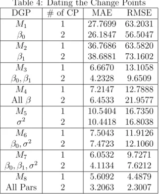
For each of the 100 repetitions we consider two measures of accuracy, mean absolute error (MAE), and root mean squared error (RMSE) defined as,
MAE = 1 100 1 W 100 X i=1 W X j=1 ¯ ¯cp j(i)−cpj(i) ¯ ¯, RMSE = v u u t 1 100 1 W 100 X i=1 W X j=1 ¡ cpj(i)−cpj(i)¢2 (20) where W is the number of change points. cpj(i) is the true position of change point j, and cpj(i) is the estimate, from the ith draw of the DGP. Recall that change points are randomly drawn from the DGP each repetition.
Table 4 reports the MAE and RMSE when the underlying process contains 1 or 2 change points. For the results to be meaningful we focus only on models which have the correct number of change points. For example, if the DGP has 2 change points, we focus on specifications that assume 2 change points only. Consistent with previous results, M1
andM2 perform the worst, and we see improvements when more parameters are subject to
structural breaks. Specification M8 in which all parameters change is the most accurate.
4.4
Sample Size
We are also concerned about the robustness of this method with respect to different sample sizes. Here we consider one of the more challenging specifications with sample sizes of 500,1000,2000 and 5000. We report results for only breaks in β1, change-point
specification M2, with 2 change points in Table 5. Increasing the number of observations
improves the identification of the true number of change points. The distribution is also more concentrated on the true model. We obtain similar, but generally better results for other models which are not reported here.
4.5
Forecasts
Another approach to compare the evidence for the number of change points is by forecast quality through the associated loss functions RMSE, MAE and theR2. TheR2 is obtained
from a regression of realized observations on a constant and a model forecast (Mincer and Zarnowitz (1969)). In our simulation exercise, we calculate these quantities as well. That is, using the change-point model estimated conditional on m −1 breaks, we calculate the in-sample model forecast for RVt using the posterior mean. Since we assume RVt is conditionally log-normal, we use the following partially analytical results for the posterior mean: E[RVt|It−1] ≈ 1 R R X h=1 exp · Xtβ(h)+ 1 2σ 2(h) ¸ (21)
where β(h), σ2(h) for h = 1, . . . , R are draws from the posterior simulator conditional on
all the data.
We calculate the in-sample RMSE, MAE and R2 for specifications M
3 and M8 and
summarize the results in Table 6. Similar results are obtained for other cases. For each criteria we report the number of times out of 100 repetitions that the specific change-point model is selected as best based on a forecast criterion and the marginal likelihood. For instance, in the top row, given a DGP with no change points, 90 out of 100 (90/100) repetitions the no change-point model has the smallest MAE, while 6/100 times the 1 change-point model is best, and 4/100 times the 2 change-point model is best. If there were perfect classification the bold numbers should be 100.
The RMSE criterion generally identifies the correct number of structural breaks. The MAE deteriorates with more change points for M3. Note that the posterior mean is
only an optimal estimate for RMSE, and we include the MAE for comparison only. The R2 criterion is particularly bad in both cases. This shows that forecasts alone provide
weaker, and in the case ofR2, misleading evidence about structural breaks. The marginal
likelihood, that uses the whole distribution and hence more information, performs better. In the case of M8, we would expect the marginal likelihood to be the best since it is
it also performs well forM3 in which the variance is not subject to breaks.
In conclusion, we have presented simulation evidence that the Chib change-point model performs well in identifying the number of structural breaks, dating change points, and the superiority of the marginal likelihood criterion in identifying the number of breaks.
5
Application to S&P 500 Volatility
5.1
Data
We consider the S&P 500 index by using the Spyder (Standard & Poor’s Depository Receipts), which is an Exchange Traded Fund that represents ownership in the S&P 500 Index. The ticker symbol is SPY. Since this asset is actively traded, it avoids the stale price effect of the S&P 500 index.9 The Spyder trades at about 1/10th the value of the
index. There is a very close correspondence between the series and generally the tracking error is well below 1%.
The Spyder price transaction data are obtained from the Trade and Quotes (TAQ) database. We removed any price transaction change that was larger than 3% which were obvious errors and keep those records with a TAQ correction indicator of 0 (regular trade) and when possible a 1 (trade later corrected). We also excluded any transaction with a sale condition of Z, which is a transaction reported on the tape out of time sequence. A 5 minute grid from 9:30 to 16:00 was constructed using previous-tick method10which means
if there is no transaction at that time grid, the nearest previous transaction record is used. The first observation of the day occurring just after 9:30 was used for the 9:30 grid time. From this grid, 5 minute intraday log returns are constructed. Then the return data was used to construct daily returns, realized volatility, and realized bipower variation. The data ranges from January 29, 1993 to March 30, 2004. Conditioning on the first 22 observations, we have T = 2791 observations. Table 7 displays summary statistics for dailyRVt and log(RVt).
5.2
Results
To conduct Bayesian estimation we use the same prior11 as in our simulation exercises
but focus on the HAR model with jumps and asymmetric terms, see equation (7). We investigate this model under the structural change configurations in Table 1. Table 8
9See Atchison et al. (1987) for a discussion of the spurious autocorrelation in index returns due to
nonsynchronous trading.
10For this and other sampling methods see Hansen and Lunde (2006).
displays the log marginal likelihood for specifications with no change point up to 7 change points.
The results suggest the existence of a change point for S&P 500 data. The log marginal likelihood for no change point is −2333.28, but all specifications with structural breaks improve on this except for M1 and M2. The difference in the best structural break
specification (M5, and one break) and the no-break model is large with a Bayes factor
of exp(57.99) in favor of a single break. This is very strong evidence. Taking a closer look at the table, the results suggest one change point. For most model settings, the largest marginal likelihood occurs at 1 change point. There is some posterior support for 2 change points for M5, but it is dominated by its 1 change point counterpart, and the
Bayes factor is 29.67 favoring 1 change point versus 2.
More interesting findings come from the comparison between models. The largest log marginal likelihood across all models is −2275.29 from M5 with 1 change point. This is
a structural break in σ2. Considering the second largest number in this table, which is
−2277.51 fromM7 with 1 change point, the Bayes factor forM5 vs M7 is 9.22. Therefore,
we conclude the effect of the break is mainly variance, but there is the possibility that the break affects the first 2 regression parameters as well as the variance of log-realized volatility.12 Our results also suggest that there is no structural break in β
2 orβ3, which
can be seen from the relative small value forM4 (compared to M3) and M8 (compared to
M7).
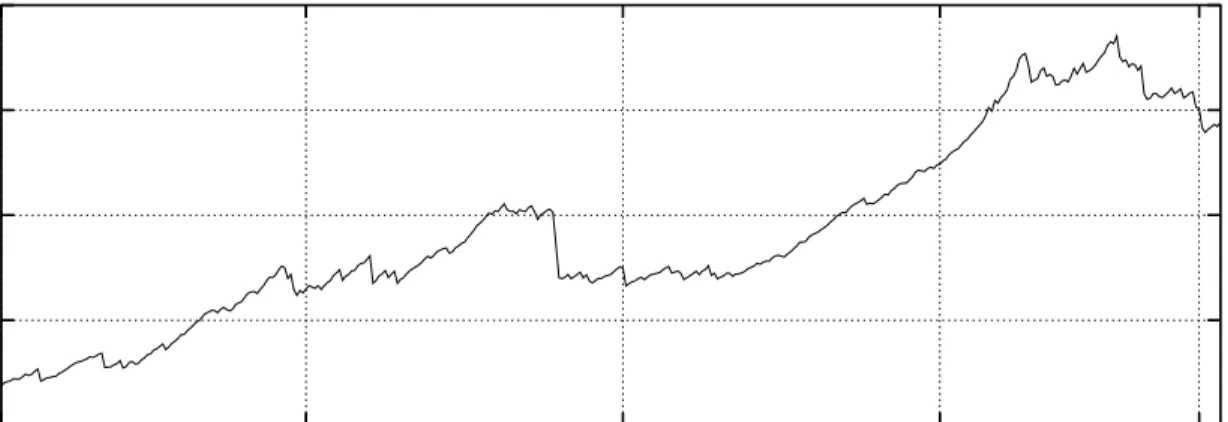
Figure 1 displays the data, the posterior density of the change point date and the cumulative probability of the change point forM5 conditional on one change point. There
is some uncertainty as to the change point date. The posterior mode of the change point density is associated with February 6, 1997.
There are several events that may have contributed to the change in volatility dynam-ics. The New York Stock Exchange (NYSE) launched real-time stock tickers on CNBC and CNN-FN in 1997. Previously, market data had been delayed 20 minutes. The NYSE changed the smallest price increment to 1/16 from 1/8 in June 1997.13 Finally, the East
12InM
7 with 1 change point, β0 goes from−0.4341, (st= 1) to −0.0971, (st= 2), and β1 goes from
0.1202 (st = 1) to 0.3089, (st = 2), and σ2 goes from 0.4581, (st = 1) to 0.2395 (st = 2). This is an
increase in the long-run mean of log-RV along with a reduction in the variance of the innovations to log-RV.
13The empirical evidence shows that the smaller ticker size resulted in a smaller bid-ask spread, but
there is no conclusive evidence about the relationship between the tick size and trading costs. Goldsteina and Kavajecz (2000) argue both spreads and depths declined after the change of the tick size, and the combined effect of smaller spreads and reduced cumulative limit order book depth has made those investors trading small orders better off. Similarly, Portniaguina et al. (2006) demonstrate trading cost are minimized at larger tick sizes for larger market orders, creating an incentive to submit smaller orders when tick size is reduced. As a result, investors will tend to submit smaller orders and execute their order patiently after the reduction in tick size.
Asian financial crisis began in the summer of 1997.
The first section of Table 9 list the posterior mean and 95% density intervals for the stable model and the best modelM5 with 1 structural break. None of the density intervals
for the parameters include 0 except for the coefficient on √|rt−1|
RVt−1. The jump coefficient is
negative, and means that a jump this period will cause log-volatility to revert to a lower level next period. In other words, volatility is less persistent after a jump. The coefficient on √|rt−1|
RVt−1I(rt <0) is positive and very large with a value of 0.2583. A negative return
leads to higher log-volatility the next day, while a positive return has little to no effect. Figure 2 plots the marginal posterior densities for the variance. There is considerable difference in the variances from the two regimes. Marginal posterior densities for other parameters are bell shaped.
5.3
Forecasts
Structural breaks can have an important effect on forecasting. In this section, we compare the predictive likelihood of the modelM5 with 1 structural break and the model without
structural breaks. The predictive likelihood contains the out-of-sample prediction record of a model, making it the central quantity of interest for model evaluation (Geweke and Whiteman (2005)).
Given the data up to time s − 1, Ys−1 = {y1, ..., ys−1}, the predictive likelihood
p(ys, ..., yt|Ys−1) (Geweke (1995,2005)) is the predictive density evaluated at the realized
outcome ys, ..., yt, s≤t. The predictive likelihood for modelA can be calculated by
p(ys, ..., yt|Ys−1, A) =
p(y1, ..., yt|A) p(y1, ..., ys−1|A)
(22) where the nominator and the denominator at the right hand side are the marginal likeli-hood for all the dataYt, and for the in-sample dataYs−1, respectively. In a similar fashion
to the Bayes factor which is based on all the data, we can compare the performance of models on a specific out-of-sample period by predictive Bayes factors. The predictive Bayes factor for model A versus B is
P BF =p(ys, ..., yt|Ys−1, A)/p(ys, ..., yt|Ys−1, B). (23)
and summarizes the relative evidence of the two models over the out-of-sample data ys, ..., yt.
To compare the out-of-sample density forecasts of the model with and without a structural break, we calculate the predictive Bayes factor for data after the break point
February 6, 1997. In other words, s−1 = February 5, 1997, and t ≥s. Specifically, for one observation (t= s) out-of-sample, P BF = 1.12; 1 month (t =s+ 21) P BF = 2.17; 3 months (t=s+ 65) P BF = 20.02; and 5 months (t=s+ 109)P BF = 176.49; each in favor of the break specification. The improvements continue till the end of sample.
5.4
Identifying the Structural Break in Real Time
To investigate how quickly we can identify the structure break, we re-estimate the model using data up to the date of the identified structural break, Feb. 6, 1997, then using data up to Feb. 7, 1997, etc. For each run, the Bayes factor is computed for the 1 change-point model M5 versus the stable no-break model.14 The recursive log(BF) is shown in
Figure 3. For the S&P 500 data, it takes 300 observations (around 14 months) to provide compelling evidence for a structural break. After this the evidence for a break continues to grow till the finalBF at the end of the sample (not shown in the figure) is exp(57.99).
5.5
Jumps and Asymmetric Terms
Our finding of a structural break is robust to the inclusion or exclusion of jumps and asymmetric terms. Table 10 reports results for our favored specification. The candi-date models include a model with neither jump nor asymmetric terms (“No jump, No Asym” column), a model with only jumps (“with Jumps” column), a model with only asymmetric terms (“with Asym” column) and a model with both jump and asymmetric terms (the last column). We also consider a model with an alternative asymmetric term log(RVt−1)I(rt−1 <0), whose results are listed in the “with Alt-Asym” column.
Accord-ing to log-marginal likelihood, the best candidate model M5 contains both jumps and
asymmetric terms. Note that the evidence for a single break is still strong in the other model formulations.
Although jumps are less significant, the asymmetric terms are very important. In-cluding them increases the marginal likelihood greatly. Nevertheless, the best model for log(RVt) is the structural break model with both jumps and asymmetric terms.
5.6
Robustness of Minimum Regime Duration
To test the robustness of the minimum regime duration, we estimate the preferred model M5 with different minimum regime lengths. The results are listed in Table 11. Besides
14The Bayes factor computed here provides a measure of the model fit to the databefore and afterthe
break point. The predictive Bayes factor in Section 5.3 provides a measure of the model fit only to data
the minimum 66 observations (3 months) setting in our previous sections, we also con-sider the minimum length as short as 10 observations (2 weeks) or 22 observations (1 month), and the longer setting of 132 observations (6 months). In this table, the first row (“Minimum Length” row) reports the lowest bound for the number of the observations in each regime. The marginal likelihoods are almost identical across the different cases. Each of the different regime duration restrictions favor the 1 change point which has a mode at February 6, 1997. The choice of the minimum regime length has little effect on our results.
5.7
The Relationship between Structural Breaks and GARCH
Effects
The change in the variance of log-volatility is related to the recent finding of heteroskedas-ticity in models of S&P 500 realized volatility (Corsi et al. (2005), Andersen et al. (2007), Bollerslev et al. (2007)).15 To investigate if our finding of a break is spurious due to
ne-glected conditional variance dynamics, we consider breaks in a HAR-GARCH model. Based on the previous results we focus on breaks in the conditional variance only. The HAR model extended to include a GARCH structure is
yt = Xtβ+γstσtut, ut ∼N(0,1) (24)
σ2
t = ω+a(yt−1−Xt−1β)2+bσt2−1, (25)
where γst is a scaling constant which has a direct effect on the unconditional variance of
log-RV. We normalizeγ1 = 1 and assume allγk >0, k = 2, ..., m. Thus, in regime 1, this is a standard HAR model with a GARCH conditional variance. While in later regimes, the conditional variance of log-RV can be larger or smaller than σ2
t depending on γst >1 or
γst <1. The advantage of this parameterization is that we can model permanent changes
in the variance but avoid the path dependence in the conditional variance16 induced by
parameter changes in ω, a, and b. As a result, the efficient full block Gibbs sampling for S|P,Θ, IT is still available.
The estimation process is more involved than the HAR model. Denoting the model parameters Θ = {β, ω, a, b, γ2,· · · , γm}, the Gibbs sampler requires us to iterate on 1)
15Both Corsi et al. (2005) and Bollerslev et al. (2007) use S&P 500 index futures over 1985-2004,
while Andersen et al. (2007) use the shorter sample 1990-2005. Corsi et al. (2005) model GARCH effects for the variance of √RVt while Bollerslev et al. (2007) model GARCH effects in the variance of the
log(RBPt), and Andersen et al. (2007) similarly model log(RBPt) adjusted by a testing procedure for
jumps.
S|P,Θ, IT, 2) P|S,Θ, IT, and 3) Θ|S, P, IT. The first and second sampling steps are identical to the basic HAR model. However, Gibbs sampling is not available for all parameters of Θ|S, P, IT. Therefore, we adopt a random walk Metropolis-Hastings (M-H) algorithm to sample Θ. The details of the estimation and calculation of the marginal likelihood are presented in the appendix. In estimation the restrictionsω >0,a≥0, b≥0, are imposed for positivity of variance and a+b <1 for stationarity.
Given our previous results, we concentrate on a stable HAR-GARCH model as well as its structural break versions with 1–3 change points. The log marginal likelihood for both the HAR model and the HAR-GARCH model are listed in Table 12. Incorporating GARCH effects, improves the model with the log (ML) increasing from−2333.28 for the stable HAR to −2276.10 for the stable HAR-GARCH parameterization. The best HAR model with constant variance within regimes and 1 change point is still marginally better than the stable HAR-GARCH model. In other words, a single structural break in the homoskedastic model provides a similar description of the data as the stable GARCH model.
There is strong evidence of parameter change for the HAR-GARCH model. Condi-tional on 1 break, the log (ML) increases from−2276.10 to −2253.38,providing a Bayes factor of exp(22.72) in favor of 1 structural break. This is consistent with our previous results. For instance, the unconditional variance of log-RV drops from 0.4482 to 0.2627 in the second regime.17 The posterior mode of the change point is exactly the same
date, February 6, 1997. Finally, there is some evidence of multiple breaks in this model. Bayesian model averaging could be used to provide forecasts that incorporate uncertainty about the number of change points.
The parameter estimates of the HAR-GARCH specification are listed in Table 9. The most notable change is the dramatic reduction in the persistence measure a+b of the conditional variance. This drops from 0.9856 for no change point, to 0.6874 for 1 change point. Not only does the no break HAR-GARCH model have the wrong long-run variance, but it also overstates the persistence of the variance of log-RV.
6
Summary and Conclusion
This paper explores structural breaks in realized volatility. We focus on the popular heterogeneous autoregressive (HAR) models of the logarithm of realized volatility (log-RV) and test for breaks using Bayesian methods. Our Monte Carlo simulations demonstrate that this method is powerful in detecting and dating structural breaks. We show that
17The unconditional variance within a regime isγ2
detecting breaks using traditional forecast criteria may be misleading. Applying our model to daily S&P 500 data, we find strong, robust evidence of a structural break in log-RV. The main effect of the break is on the variance of log-volatility, but there is weaker evidence for a change in both the regression parameters and variance. We demonstrate that accounting for the structural break improves density forecasts. Finally, we consider a HAR model with GARCH effects and also find a structural break in the unconditional variance of log-RV. There is a permanent reduction in the variance of log-RV in February 1997 for all of our specifications using data from 1993-2004. Failure to model this break results in biased parameter estimates and poor density forecasts.
7
Appendix
7.1
Marginal Likelihood
In this appendix we review the estimation of the marginal likelihood following Chib (1995). Given observations YT ={y1, y2, . . . , yT}, we follow the notation in the previous sections except that conditioning on Xt is suppressed. A rearrangement of Bayes rule gives the marginal likelihood, p(YT), as
p(YT) = f(YT|Θ, P)p(Θ, P) p(Θ, P|YT)
(26) wheref(YT|Θ, P) is the likelihood function, p(Θ, P) is the prior density andp(Θ, P|YT) is the posterior ordinate. Although this equation is valid for any value (Θ, P) in the parameter space, a point with high posterior mass will tend to provide a more accurate estimate. Therefore, we select the posterior mean denoted as (Θ∗, P∗). Then
lnp(YT) = logf(YT|Θ∗, P∗) + logp(Θ∗, P∗)−logp(Θ∗, P∗|YT) (27)
The prior densityp(Θ∗, P∗) can be evaluated directly and the likelihood functionf(Y
T|Θ∗, P∗) can be calculated as in (18).
To calculate the posterior ordinate p(Θ∗, P∗|Y
T), note the decomposition p(Θ∗, P∗|Y T) = p(β∗|YT)p ¡ σ2∗|Y T, β∗ ¢ p¡P∗|Y T, β∗, σ2∗ ¢ (28) where each term on the right hand side can be estimated from MCMC simulations. The first term is,
p(β∗|YT) = Z p¡β∗|YT, S, σ2 ¢ p¡S, σ2|YT ¢ dSdσ2 (29)
and can be estimated as \ p(β∗|YT) = 1 R R X h=1 p¡β∗|YT, σ2(h), S(h)¢ (30)
where the draws {σ2(h), S(h)}R
h=1 are available directly from our estimation step, and
p¡β∗|YT, σ2(h), S(h)¢ = Qm k=1p ¡ β∗ k|YT, σ2(h), S(h) ¢
where each conditional density is de-termined by (16). The second term in (28) is equal to
p¡σ2∗|Y T, β∗ ¢ = Z p¡σ2∗|Y T, β∗, S ¢ p(S|, YT, β∗)dS, (31) wherep(σ2∗|YT, β∗, S) =Qm
k=1p(σ2k∗|YT, β∗, S) and each conditional posterior has density according to (17). To obtain the draws from p(S|YT, β∗), we run an additional reduced Gibbs sampling conditional onβ∗; i.e. we run all the sampling in Section 3.1 except that
we do not draw the values forβ but fix them to beβ∗. From this reduced run simulation,
{S(h)}R h=1 is used in \ p(σ2∗|Y T, β∗) = 1 R R X h=1 p¡σ2∗|Y T, β∗, S(h) ¢ . (32)
The last term of (29) is
p¡P∗|Y T, β∗, σ2∗ ¢ = mY−1 i=1 p¡p∗ ii|YT, β∗, σ2∗ ¢ (33) and each term equal to
p¡p∗ii|YT, β∗, σ2∗¢=
Z
p¡p∗ii|YT, S, β∗, σ2∗¢p¡S|β∗, σ2∗, YT¢dS
Sampling {S(h)}R
h=1 fromp(S|β∗, σ2∗, YT) the estimate of each term is
\ p(p∗ ii|YT, β∗, σ2∗) = 1 R R X h=1 p¡p∗ ii|YT, S(h), β∗, σ2∗ ¢ . (34)
7.2
Estimation of HAR-GARCH model
We set all priors in the regression equation as before, they are independent normal N(0,100). The GARCH parameters have independent normal N(0,100) truncated to ω >0, a≥0, b ≥0, anda+b <1. The priors for the scaling parametersγk(k = 2,· · · , m)
are also truncatedN(0,100) with positive supports. These priors are uninformative. For the sampling step Θ|S, P, IT, the conditional distributions for some of the model parameters are unknown, and therefore Gibbs sampling is not available. Instead we use a random walk Metropolis-Hastings algorithm. If we denote all the parameters except for θl as Θ−l ={θ1,· · · , θl−1, θl+1,· · · , θL}, we sample a new θl given Θ−l fixed. With Θ as the previous value of the chain we iterate on the following steps:
Step 1: Propose a new Θ0 according to Θ0−l= Θ−l, with element l determined as
θ0
l=θl+el, el ∼N(0, ξl2). (35)
Step 2: Accept Θ0 with probability min ½ p(YT|Θ 0 , P, S)p(Θ0, P) p(YT|Θ, P, S)p(Θ, P) ,1 ¾ (36) and otherwise reject. p(Θ, P) is the prior, and
logp(YT|Θ, P, S) = T X t=1 · −1 2log(2π)− 1 2log(γ 2 stσ 2 t)− (yt−Xtβ)2 2γ2 stσ 2 t ¸ (37) where σ2
t = ω +a(yt−1 −Xt−1β)2 +bσt2−1.18 Each ξl2 is selected to give an acceptance frequency between 0.3–0.5. Running Step 1-2 above for all the parameters l = 1,· · · , L, we obtain a new draw Θ which is one iteration. We perform 200,000 iterations and use the last 100,000 for posterior inference.
For the marginal likelihood we use the method of Gelfand and Dey (1994) adapted by Geweke (2005) (Section 8.2.4). This estimate is based on 1
R
PR
h=1g(Θ(h))/[p(YT|Θ(h), P(h))p(Θ(h), P(h))]→ p(YT)−1 as R → ∞, where p(YT|Θ, P) is the likelihood with S integrated out as in
(18)-(19), andg(Θ(h)) is a truncated multivariate Normal. Note that the prior, likelihood and
g(Θ) must contain all integrating constants. Finally, to avoid underflow/overflow we use logarithms in this calculation and above in (36).
References
[1] Andersen, T. G. and T. Bollerslev. (1998). “Answering the Skeptics: Yes, Standard Volatility Models Do Provide Accurate Forecasts.” International Economic Review,39, 885-905.
18To start up the conditional variance we setσ2
[2] Andersen, T. G., T. Bollerslev and F. X. Diebold. (2006). “Roughing It Up: Including Jump Components in the Measurement, Modeling and Forecasting of Return Volatility.”Review of
Economics and Statistics, forthcoming.
[3] Andersen T. G., T. Bollerslev, F. X. Diebold and H. Ebens. (2001). “The Distribution of Realized Stock Return Volatility.” Journal of Financial Economics, 61, 43-76.
[4] Andersen T. G., T. Bollerslev, F. X. Diebold and P. Labys. (2001). “The Distribution of Exchange Rate Volatility.” Journal of the American Statistical Association, 96, 42-55. [5] Andersen T. G., T. Bollerslev, F. X. Diebold and P. Labys. (2003). “Modeling and
Forecast-ing Realized Volatility.”Econometrica 71.2, 579-625.
[6] Andersen, T. G., T. Bollerslev and X. Huang. (2007). “A Reduced Form Framework for Modeling Volatility of Speculative Prices based on Realized Variation Measures.” Working paper, Duke University.
[7] Andreou, E. and E. Ghysels. (2002). “Detecting Multiple Breaks in Financial Market Volatil-ity Dynamics.”Journal of Applied Econometrics, 17(5), 579-600.
[8] Atchison, M. D., K. Butler and R. R. Simonds. (1987). “Nonsynchronous Security Trading and Market Index Autocorrelation.”The Journal of Finance, 42(1), 111-118.
[9] Bandi F. M. and J. R. Russell. (2006). “Separating Microstructure Noise from Volatility.”
Journal of Financial Economics, 79, 655-692.
[10] Barndorff-Nielsen O. E. and N. Shephard. (2002a). “Econometric Analysis of Realized Volatility and its Use in Estimating Stochastic Volatility Models.” Journal of the Royal
Sta-tistical Society, Series B, 64, 253-280.
[11] Barndorff-Nielsen O. E. and N. Shephard. (2002b). “Estimating Quadratic Variation using Realised Variance.”Journal of Applied Econometrics, 17, 457-477.
[12] Barndorff-Nielsen O. E. and N. Shephard. (2004). “Power and Bipower Variation with Stochastic Volatility and Jumps.” Journal of Financial Econometrics, 2(1), 1-37.
[13] Bauwens, L., A. Preminger and J. V.K. Rombouts. (2006). “Regime Switching GARCH Models.” CORE Discussion paper 2006/11.
[14] Bollerslev, T., U. Kretschmer, C. Pigorsch and G. E. Tauchen. (2007). “A Discrete-Time Model for Daily S&P 500 Returns and Realized Variations: Jumps and Leverage Effects.” working paper, Duke University.
[15] Chib, S. (1995). “Marginal likelihood from the Gibbs output.” Journal of the American
[16] Chib, S. (1996). “Calculating Posterior Distributions and Modal Estimates in Markov Mix-ture Models.” Journal of Econometrics, 75, 79-97.
[17] Chib, S. (1998). “Estimation and comparison of multiple change point models.”Journal of
Econometrics, 86, 221-241.
[18] Chib, S. (2001). “Markov Chain Monte Carlo Methods: Computation and Inference.” In J.J. Heckman and E. Leamer (eds.), Handbook of Econometrics, volume 5, North Holland, Amsterdam, 3569-3649.
[19] Chu, CS J. (1995). “Detecting Parameter Shift in GARCH Models.”Econometric Reviews, 14, 241-266.
[20] Corsi, F. (2004). “A simple long memory model of realized volatility.” Working paper, University of Southern Switzerland.
[21] Corsi, F., U. Kretschmer, S. Mittnik and C. Pigorsch. (2005). “The Volatility of Realized Volatility.” Center for Financial Studies, working paper 2005/33.
[22] Engle, R. F. and J. G. Rangel. (2005). “The Spline-GARCH Model for Unconditional Volatility and its Global Macroeconomic Causes.” Working Paper, New York University and UCSD.
[23] Forsberg, L. and E. Ghysels. (2006). “Why do Absolute Returns Predict Volatility so well.” working paper, University of North Carolina, Chapel Hill.
[24] Gelfand, A. and D. Dey. (1994). “Bayesian Model Choice: Asymptotics and Exact Calcu-lations.” Journal of The Royal Statistical Society, B, 56,501-514.
[25] Geweke, J. (1992). “Evaluating the accuracy of sampling-based approaches to calculating posterior moments (with discussion).” In J.M. Bernardo, J.O. Berger, A.P. Dawid and A.F.M. Smith (eds.), Bayesian Statistics, Vol. 4, 169-193, Oxford: Oxford University Press.
[26] Geweke J. (1995). “Bayesian comparison of Econometric Models.” Working paper, Research Department, Federal Reserve Bank of Minneapolis.
[27] Geweke J. (2005).Contemporary Bayesian Econometrics and Statistics. John Wiley & Sons Ltd.
[28] Geweke J. and C. Whiteman. (2005). “Bayesian Forecasting,” Forthcoming in Handbook of Economic Forecasting, Edited by Elliott, Granger and Timmermann, Elsevier.
[29] Ghysels, E., P. Santa-Clara and R. Valkanov. (2003). “Predicting Volatility: Getting the Most out of Return Data Sampled at Different Frequencies.”Journal of Econometrics (forth-coming).
[30] Giot P. and S. Laurent. (2004). “Modelling daily Value-at-Risk using realized volatility and ARCH type models.”Journal of Empirical Finance, 11, 379-398.
[31] Giot P. and S. Laurent. (2006). “The information content of implied volatility in light of the jump/continuous decomposition of realized volatility.” Journal of Futures Markets, forthcoming.
[32] Goldsteina, M. A. and K. A. Kavajecz. (2000). “Eighths, sixteenths, and market depth: changes in tick size and liquidity provision on the NYSE.” Journal of Financial Economics, 56, Issue 1, April 125-149.
[33] Hamilton, J. D. (1989). “A New Approach to the Economic Analysis of Nonstationary Time Series and the Business Cycle.” Econometrica, Vol. 57, No. 2, 357-384.
[34] Hansen P. R. and A. Lunde. (2006). “Realized Variance and Market Microstructure Noise.”
Journal of Business and Economic Statistics, 24, 127–218.
[35] Hillebrand, E. (2005). “Neglecting parameter changes in GARCH models.” Journal of
Econometrics, 127 (1-2), 121-138.
[36] Huang, X. and G. Tauchen. (2005). “The Relative Contribution of Jumps to Total Price Variance.”Journal of Financial Econometrics, 3, 456-499.
[37] Hwang, S. and P. L. V. Pereira. (2004). “The Effects of Structural Breaks in ARCH and GARCH Parameters on Persistence of GARCH Models.” working paper, Cass Business School.
[38] Kass, R. E. and A. E. Raftery. (1995). “Bayes factors and model uncertainty.”Journal of
the American Statistical Association, 90, 773-795.
[39] Kim, C-J., J. C. Morley and C. Nelson. (2005). “The Structural Break in the Equity Premium.” Journal of Business and Economic Statistics, 23(2), 181-191.
[40] Koop G. and S. M. Potter. (2004). “Prior Elicitation in Multiple Change-point Models.” Working Paper, University of Strathclyde.
[41] Koopman, S. J., B. Jungbacker and E. Hol. (2005). “Forecasting daily variability of the S&P 100 stock index using historical, realised and implied volatility measurements.” Journal
of Empirical Finance, 12(3), 445-475.
[42] Lamoureux, C. G. and W. D. Lastrapes. (1990). “Persistence in Variance, Structural Change, and the GARCH Model.”Journal of Business and Economic Statistics, 8(2), 225-34. [43] Maheu, J. M. and T. H. McCurdy. (2002). “Nonlinear Features of Realized FX Volatility.”