Human Development
Research Paper
2010/24
Determinants of Human
Development: Insights from
State-Dependent Panel Models
Michael Binder
and Georgios Georgiadis
United Nations Development Programme
Human Development Reports
Research Paper
September 2010
Human Development
Research Paper
2010/24
Determinants of Human
Development: Insights from
State-Dependent Panel Models
Michael Binder
and Georgios Georgiadis
U
nited Nations Development Programme
Human Development Reports
Research Paper 2010/24
September 2010
Determinants of Human Development:
Insights from State-Dependent Panel Models
Michael Binder
and Georgios Georgiadis
Michael Binder is Professor of International Macroeconomics and Macroeconometrics at Goethe University Frankfurt and Director of the Policy Research Network of the Graduate School of Economics, Finance, and Management at Goethe University, Johannes Gutenberg University Mainz and Technical University Darmstadt and
the Center for Financial Studies. E-mail: [email protected].
Georgios Georgiadis is a Ph.D. candiadate at the Graduate School of Economics, Finance, and Management at Goethe University, Johannes Gutenberg University Mainz and Technical University Darmstadt. E-mail:
Abstract
In this paper, we study economic development in a panel of 84 countries from 1970 to 2005. We focus on characterizing heterogeneities in the development effects of macroeconomic policies and on comparing the development process as measured by GDP to that measured by the Human Development Index (HDI). We do so within a novel dynamic panel modelling framework that can account for crucial aspects of both the cross-sectional and intertemporal features of the observed process of economic development, and that can capture the dependence of the development effects of macroeconomic policies on differences in countries' persistent characteristics, such as their social norms and institutions. Among our findings are that macroeconomic policies affect economic development with less delay than suggested by conventional econometric frameworks, yet impact HDI with longer delay and overall less strongly than GDP. Differences in countries' persistent characteristics may even affect the sign of the long-run development effects of a given macroeconomic policy: Fiscal stimuli in the form of government consumption positively affect GDP in countries with low institutional quality, but negatively affect long-run GDP in countries with high institutional quality.
Keywords: human development, institutions and social norms, dynamic panel modelling. JEL classification: C23, O10
The Human Development Research Paper (HDRP) Series is a medium for sharing recent research commissioned to inform the global Human Development Report, which is published annually, and further research in the field of human development. The HDRP Series is a quick-disseminating, informal publication whose titles could subsequently be revised for publication as articles in professional journals or chapters in books. The authors include leading academics and practitioners from around the world, as well as UNDP researchers. The findings, interpretations and conclusions are strictly those of the authors and do not necessarily represent the views of UNDP or United Nations Member States. Moreover, the data may not be consistent with that presented in Human Development Reports.
1
Introduction
Research aimed at understanding countries’ long-run economic development has been a cornerstone of theoretical and empirical economic investigations for many decades. While substantial progress has been made during the last couple of decades, various issues re-main controversially discussed or have received attention only recently. Among these issues are in particular (i) how correlates of economic growth can be distinguished from factors that are causal for economic growth, (ii) how the contributions of key development policies to advances in economic prosperity may depend on a country’s institutions, social norms and other societal characteristics, as well as (iii) whether measures other than
out-put/income should be considered when comparing economic development across
coun-tries. In this paper, we study economic development in a panel of 84 countries from 1970
to 2005. We investigate heterogeneities in the development effects of macroeconomic
policies, and compare the development process as measured by GDP to that measured by the United Nations’ Human Development Index (HDI). We do so within a novel dynamic panel modelling framework that can account for crucial aspects of both the cross-sectional and intertemporal features of the observed process of economic development. The frame-work we propose can also characterize a possible state dependence of the development
effects of macroeconomic policies on differences in countries’ persistent characteristics,
such as their social norms and institutions as well as other key societal characteristics within which the development process takes place.
To motivate our panel modelling framework, it is useful to note that the predominant in-vestigative tool used in the empirical output growth literature continues to be the “Barro regression”, in which a country’s rate of output growth during a certain time period is re-gressed on an initial condition for the level of output and a variety of other potential output
growth determinants.1 There are a number of problems with this Barro regression
frame-work, however, which limit its usefulness for empirical analysis.2 A first issue casting
doubt on the appropriateness of the Barro regression framework is that - random effects
apart - all cross-country heterogeneities of the output growth process are assumed to be
fully captured by different realizations of the regression’s explanatory variables. This
is, however, extremely unlikely to be satisfied in practice, as due to finite sample issues only a limited number of explanatory variables - capturing only a portion of the overall
cross-country heterogeneity - can be considered, and as many of the systematic diff
er-ences prevailing across countries are difficult to observe or to measure. For this reason,
Islam (1995) and Evans (1996) were among the first in the recent empirical output growth literature to move beyond the Barro regression framework, advocating to consider panel
fixed-effects models, with the fixed effects accounting for time-invariant factors, such as
a country’s institutional and political environment, that exhibit systematic (as opposed to purely random) variation across countries. Pursuing this line of thought further, however,
not only may countries’ systematically differing societal characteristics imply different
conditional means for the steady-state distribution of the relevant development measure,
but countries may also feature different slopes of their steady-state growth paths, due to
prolonged differences, say, in the rate of technological progress. As has been argued by
Lee, Pesaran and Smith (1997) and Binder and Pesaran (1999), assuming that countries
in the steady state grow at the same rate when steady-state growth rates in fact differ,
leads to serious fallacies in empirical inference. More generally, a promising econometric
framework for studying economic development beyond allowing for fixed effects must
capture systematic heterogeneities in growth dynamics also. A second issue of concern
1This regression framework has become popular in empirical work following the seminal paper by Barro (1991).
2See also Hauk and Wacziarg (2009) for a recent discussion of some of these issues. In this paper we take a different perspective than Hauk and Wacziarg (2009), however, by arguing in favor of a dynamic panel model-based inference approach as being the appropriate means for the cross-country econometric analysis of economic development.
with default Barro regressions is that they are subject to endogeneity bias. Regressions of, say, output growth on a variable such as the rate of investment in physical capital that a priori postulate investment in physical capital to be exogenous may help one to understand the strength of the association of output growth with investment in physical capital, but cannot provide evidence as to whether investment in physical capital is in fact a determinant of a country’s rate of output growth in the sense that a higher rate of invest-ment in physical capital would precede accelerated output growth (as it may well be that a higher rate of investment in physical capital merely is a result of higher output levels
and/or higher output growth rates). For purposes of policy analysis, it is clearly desirable,
however, to work with an econometric framework that can distinguish between correlates
and determinants of economic growth.3 Third in terms of concerns with the Barro
re-gression framework is that it does not feature a data-driven distinction between short- and long-run dynamics, and is not designed to deal with the possible presence of unit roots in the data and resulting issues of non-ergodicity (see Binder and Pesaran, 1999). Fourth and finally, there is mounting evidence that the process of economic development is subject
to important nonlinearities, such as the dependence of the development effects of
macroe-conomic policies on country-specific conditions. Such nonlinearities are not captured by default Barro regressions. See, for example, Rodr´ıguez (2007) and Binder, Georgiadis and Sharma (2010). Taking all four of these issues together, there appears to be a clear need for empirical work on economic development to move beyond econometric techniques as typically used in the empirical output growth literature.
Beyond giving careful consideration to econometric modelling issues, in this paper we
also go beyond a strictly output-/income-based analysis of the development process. As
prominently advocated by Sen (1999), the ultimate goal of economic development poli-cies should be to enhance - in a rather broad sense - the set of people’s opportunities.
3We should mention that there is important work tackling this endogeneity issue within the framework of Barro regressions. See, for example, Acemoglu, Johnson and Robinson (2001).
The empirical growth literature to date has, however, primarily focused on investigating the determinants of the level of output (income) per capita and its growth rate. While it
is obviously true that a higher level of output/income can afford an expanded set of
con-sumption goods, the focus of the empirical growth literature on output/income measures
might cloud other key aspects of the complete set of opportunities available to individuals, as eminently described in the first Human Development Report in 1990:
First, national income figures, useful though they are for many purposes, do not reveal the composition of income or the real beneficiaries. Second, people often value achievements that do not show up at all, or not immediately, in higher measured income or growth figures: Better nutrition and health ser-vices, greater access to knowledge, more secure livelihoods, better working conditions, security against crime and physical violence, satisfying leisure hours, and a sense of participating in the economic, cultural and political activities of their communities. Of course, people also want higher incomes as one of their options. But income is not the sum total of human life.
It therefore appears to be sensible to consider replacing/augmenting output as the sole
measure of economic development by an alternative measure that shifts the focus of
de-velopment economics from solely output-oriented to human-life-oriented policy design.4
Taking into account both these econometric and data-measurement considerations, in this paper, then, we move beyond a Barro regression based analysis of output growth. We take advantage of newly released United Nations HDI data, and examine some key as-pects of these (as well as GDP) data within a novel dynamic panel modelling framework. In particular, we adapt a panel autoregressive distributed lag model with conditionally
ho-mogenous (state-dependent) long-run coefficients, as proposed by Binder and Offermanns
4We follow the lead of work in the United Nations Development Program, for example Gray Molina and Purser (2010), in moving beyond output-based development analysis.
(2007) as well as Binder, Georgiadis and Sharma (2010). The conditional pooled mean group (CPMG) state-dependent panel model introduced in these papers appears to be well-suited for the analysis of the determinants of HDI, as it can capture crucial aspects of both the cross-sectional as well as intertemporal features of the HDI development process, and can overcome the problems associated with the Barro regression approach detailed above. In particular, the CPMG state-dependent panel model (i) features a data-driven dis-tinction between short- and long-run dynamics, (ii) allows for systematic cross-country heterogeneity in intercepts and dynamics while also identifying features of the develop-ment process that are common across countries, (iii) allows for the explanatory variables to be potentially endogenous, and (iv) remains applicable even when there are unit roots in the data. Perhaps most importantly, however, the CPMG state-dependent panel model
allows us to investigate whether the development effects of changes in macroeconomic
policies on HDI (GDP) vary across different types of societal environments within which
the development process takes place. Modelling the development effects that
macroeco-nomic policies have on HDI (GDP) as being dependent on slowly time-varying indices measuring countries’ persistent characteristics appears to be a novel and promising way to
reconcile a fixed effects empirical growth model with an analysis of social norms,
institu-tions and other societal characteristics that are typically emphasized in empirical analyses
using the (random effects based) Barro regression framework.5 In this spirit, our approach
to modelling state dependence of the development effects of macroeconomic policies
in-volves modelling these effects as a function of indices involving grouped combinations of
variables that in the recent empirical growth literature have been found to robustly affect
output growth.
The plan for the remainder of this paper is as follows: In Section 2, we provide some stylized facts about the HDI development process, contrasting it to that for GDP. In
Sec-5It is important to recall that in a fixed effects panel data model one cannot identify the effects of strictly time-invariant regressors.
tion 3, we discuss our panel modelling framework, putting emphasis on how our model
in a novel form captures both country fixed effects and the cross-country variation of the
development effects of economic policies along countries’ persistent characteristics such
as its social norms and institutions. We also discuss our set of state variables measuring such persistent characteristics in Section 3. In Section 4, we present our main empirical results, contrasting these results to those we obtain for our data from conventional Barro regressions. We conclude in Section 5, also indicating some directions for future research.
Several appendices provide details on data measurement and computational/econometric
issues.
2
Some Stylized Facts About HDI Trends
While the (to date) official United Nations data for HDI are available only from 1980
onwards and for a total of 82 countries, the Gray Molina and Purser (2010) HDI data set that we can take advantage of in this paper significantly expands HDI data coverage both across years and countries: The Gray Molina and Purser (2010) data set spans 111
countries from 1970 to 2005.6 We focus in this paper on those of these 111 countries
6It may be useful to briefly recall the measurement of HDI: HDI is constructed as an index aggregat-ing information on the stage of human development as contained in GDP per capita, life expectancy, and education as measured by school enrolment and the adult literacy rate. Denoting by gd p∗
itthe logarithm of GDP per capita, by li f e∗
itlife expectancy at birth, by tgerit the tertiary gross enrolment rate, and by literit the adult literacy rate, HDI by the United Nations is computed as follows:
hdiit = 1 3 ·gd pit+ 1 3·li f eit+ 1 3·educit, (1) where educit = 1 3·tgerit+ 2 3 ·literit,
and with two of the components of HDI being re-scaled prior to entering on the right-hand side of Equation (1), so as to fall into the unit interval, [0,1]:
li f eit= li f e∗
it−25
for which there is a sufficient number of time-series observations available for them to be included in the estimation of our state-dependent panel model, leaving us with a “world”
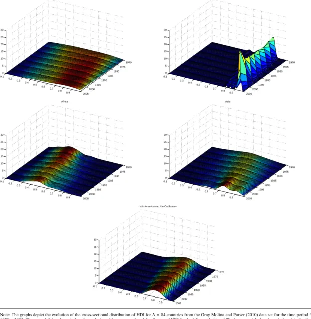
sample of 84 countries.7 Figure 1 provides the evolution of key first and second moments
of the cross-sectional distributions of HDI for subsets of countries, and Figure 2 plots the evolutions of the cross-sectional distributions themselves. When interpreting the plots (of the moments of) these distributions, it should be kept in mind that HDI and GDP per capita may not be ergodic variables - that is, they may not converge to time-invariant steady-state distributions, and second moments may not be well defined (see Binder and Pesaran, 1999). With this caveat, Figures 1 and 2 indicate that, not too surprisingly, throughout the sample period the OECD countries have enjoyed the highest levels of human development followed by countries in Latin America and the Caribbean, by countries in Asia and finally by countries in Africa. Figures 1 and 2 also suggest that unconditional convergence of HDI with respect to initial values has taken place, in the sense that HDI has generally improved relatively more in less developed regions than in the OECD countries. The median of HDI in the OECD countries from 1970 to 2005 rose by 13%, whereas it rose by 22% in Latin America and the Caribbean, by 32% in Africa, and by 32% in Asia. The most rapid catch-up with the OECD countries’ level of human development took place in Asia, for which mean (though not yet median) human development in 2005 surpassed that in Latin America and the Caribbean. Also, within each region except for Africa, the standard deviation of the cross-sectional distribution of HDI has decreased from 1970 to 2005: The standard deviation for the OECD countries from 1970 to 2005 fell by 66%, for the Latin American and Caribbean countries by 45%, and for the Asian countries by 23 %, whereas it rose for the African countries by 23%.
and
gd pit=
gd p∗it−log(100)
log(40,000)−log(100). (3)
7See Section 3 for a detailed discussion of our data availability criteria. Table 1 provides a listing of all 84 countries that enter our “world” sample.
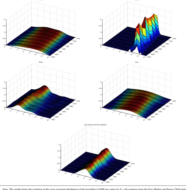
Analogously to Figures 1 and 2 for HDI, Figures 3 and 4 present the evolution of key first and second moments of the cross-sectional distributions of the logarithm of GDP per capita and the evolutions of the cross-sectional distributions themselves. Comparing Figures 3 and 4 for the logarithm of GDP per capita with Figures 1 and 2 for HDI, three observations stand out: First, while all regions have experienced notable improvements in HDI from 1970 to 2005, this is not the case for the logarithm of GDP per capita, as the mean and median of African countries’ GDP per capita have not grown in comparable magnitude as those of the OECD, Asian as well as Latin American and Caribbean coun-tries. Second, for the Latin American and Caribbean countries, the unconditional conver-gence to OECD development levels apparently present in the evolution of the mean and median of HDI does not appear to be present for the logarithm of GDP per capita. The median of the logarithm of GDP per capita in the OECD countries from 1970 to 2005 rose by 7%, whereas it rose by 6% in Latin America and the Caribbean, by 1% in Africa, and by 13% in Asia. Third, while except for Africa countries within a given region appear to unconditionally converge towards a common level of HDI, with the exception of Asia and of Latin America and the Caribbean there does not appear to be a general long-term
decline of the within-region standard deviations for the logarithm of GDP per capita.8
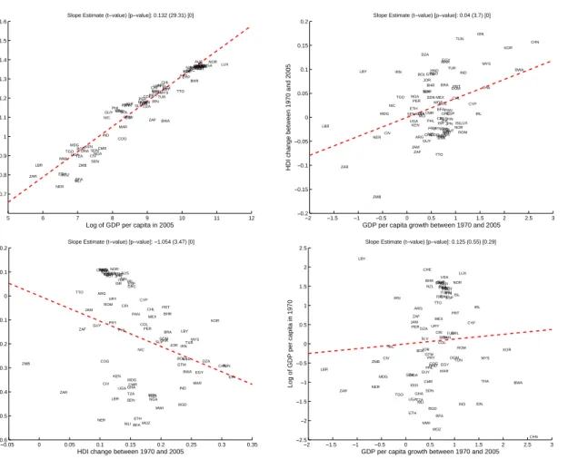
Finally in terms of stylized facts for our data, Figure 5 provides scatter plots of the HDI levels in 2005 against the logarithm of GDP per capita in 2005, of the changes in HDI against GDP per capita growth rates between 1970 and 2005, and scatter plots of the change in (growth of) HDI (GDP per capita) between 1970 and 2005 against initial HDI (GDP per capita) in 1970. Still keeping in mind the caveat that HDI and GDP per capita may not be ergodic variables, there is a strong positive correlation (with a correlation
coefficient of 0.96) between the levels of HDI and of the logarithm of GDP per capita
in 2005. The relationship between the change of HDI between 1970 and 2005 and the
8For a more detailed investigation of (unconditional) convergence of HDI and its components, see Mayer-Foulkes (2010).
growth of GDP per capita during the same time period also is positive, though with a slope only about one third as large as for the corresponding levels relationship. While there appears to be a negative and statistically significant relationship between the initial level of HDI in 1970 and the change of HDI between 1970 and 2005, pointing to the presence of unconditional convergence for HDI, the same does not appear to be the case for GDP per capita. To move beyond such a simple graphical and regression analysis inter
alia not involving any form of conditioning on country-specific characteristics and failing
to account for the possible lack of ergodicity of the levels of HDI and GDP per capita, we move to our panel-econometric analysis.
3
Econometric Model
Let us consider a panel autoregressive distributed lag model, in which we allow the key
coefficients to be state dependent, varying as a function of a (pre-determined) conditioning
state variable, zi,t−1:
yit = µi+ϕi·t+ p ! k=1 ρik(zi,t−1)·yi,t−k + q ! k=0 !#ik(zi,t−1)·xi,t−k+#it, t=r,r+1, . . . ,T, (4)
where yit denotes the dependent variable of country i at time t (hdiit or gd pit), µi and
ϕi denote fixed-effects intercept and time-trend terms, xit denotes an m × 1 vector of
explanatory variables, ρik(zi,t−1) and !#ik(zi,t−1) denote state-dependent slope coefficients,
r = max(p,q), the disturbance term #it is distributed as #it ∼ "0, σ2i#, i.i.d. across t, and
with the disturbance terms in addition being independent across i.9
9For ease of exposition we assume in Equation (4) that all explanatory variables enter with the same lag order and that the time-series dimension is the same for all countries, involving observations for yit, xitand zitfor t =0,1, . . . ,T . In our empirical work, we certainly do allow for variable- and country-specific lag
The principal idea underlying our consideration of a model with state-dependent coeffi
-cients is as follows: In the Barro regression framework, the effects of time-invariant
vari-ables on the dependent variable are identified by restricting the country-specific effects
to be random (rather than fixed) effects, imposing orthogonality between the
country-specific effects and the model’s other regressors, including those in xit. As discussed in
the Introduction, such a random effects restriction for cross-country models is
implausi-ble in empirical practice, as many of the development factors forming the country-specific
effects vary systematically (not randomly) across countries. It is thus imperative to allow
for fixed-effects intercepts, the µi’s in Equation (4). Of course, having introduced such
fixed effects, it is no longer possible to identify the effects of any other regressors that are
strictly time-invariant. Our conditioning states, the zi,t−1’s, are indices involving variables
that reflect similar aspects of a country’s institutions, social norms or other key societal
characteristics. Carefully combining such variables, we ensure that the zi,t−1’s feature
some time variation. Our model thus overcomes the implausible and costly random
ef-fects restriction of the Barro regression framework,10without having to pass on examining
the quantitative importance of a country’s institutions and aspects of its social norms for
its development process.11
The error-correction representation of Equation (4), separating short- and long-run dy-namics in a data-driven manner, is given by
∆yit= µi+ϕi·t+αi(zi,t−1)·yit−1+βi#(zi,t−1)· xi,t−1+ψ#i(zi,t−1)·hit+#it
= µi+ϕi·t+αi(zi,t−1)·$yi,t−1−θ#i(zi,t−1)·xi,t−1%+ψ#i(zi,t−1)· hit+#it, (5)
orders piand qik, for k=1,2, . . . ,m and i=1,2, . . . ,N, as well as for an unbalanced panel of observations. 10In separate simulation work in progress, we document the magnitude of the parameter estimate biases that may be incurred in the development context by erroneously modelling fixed effects as random effects.
11Due to reasons of model parsimony, we will not consider model specifications allowing for more than one conditioning state variable at a time, and will examine the influence of our set of conditioning state variables in sequential form, one state variable at a time. See Binder, Georgiadis and Sharma (2010) for a state-dependent dynamic panel data model with multivariate conditioning.
where αi(zi,t−1)= !p k=1ρik(zi,t−1)−1, βi(zi,t−1)= !q k=0!ik(zi,t−1), ψi(zi,t−1)= & −!p k=2ρik(zi,t−1),− !p k=3ρik(zi,t−1), . . . ,−ρip(zi,t−1), !#i0(zi,t−1),− !q k=2! # ik(zi,t−1),− !q k=3! # ik(zi,t−1), . . . ,−!#iq(zi,t−1) '# , hit = (
∆yi,t−1,∆yi,t−2, . . . ,∆yi,t−p+1,∆x#it,∆x
# i,t−1, . . . ,∆x # i,t−q+1 )# , and
θi(zi,t−1)=−βi(zi,t−1)/αi(zi,t−1).
Given the still relatively limited number of time-series observations typically available in cross-country development panel data sets such as the one we use for this paper, we need to restrict the degree of parameter variation allowed for by the model in Equation (5). To this end, we specify the speed of adjustment and the other model short-run dynamics as
varying in unrestricted form across countries, but not varying with zi,t−1. Also
introduc-ing the weak conditional/state-dependent pooling restriction that countries that share the
same values of the conditioning state variables also share the same long-run multipliers,
θi(zi,t−1)= θ(zi,t−1),12we then have the conditional pooled mean group (CPMG) panel data
model
∆yit = µi+ϕi·t+αi·yi,t−1+βi#(zi,t−1)·xi,t−1+ψ#i · hit+#it
= µi+ϕi·t+αi·$yi,t−1−θ#(zi,t−1)· xi,t−1%+ψ#i ·hit+#it. (6)
12The restriction thatθ
i(zi,t−1) =θ(zi,t−1), i = 1,2, . . . ,N, is obviously much weaker than the uncondi-tional generic slope coefficient pooling restriction of Barro regressions and fixed-effects panel data models, and also is significantly weaker still than the unconditional long-run pooling restriction of the pooled mean group model of Pesaran, Shin and Smith (1999), namelyθi(zi,t−1)=θ, i=1,2, . . . ,N. See Binder and
Of-fermanns (2007) and Binder, Georgiadis and Sharma (2010) for previous empirical evidence in the context of exchange rate and output growth dynamics that the weak conditional/state-dependent long-run pool-ing restriction we consider here still sizeably increases the efficiency of parameter estimates compared to country-specific time-series analyses.
In this framework featuring conditional or state-dependent long-run homogeneity, all transitional dynamics are fully country-specific, and the long-run dynamics are homo-geneous only for countries sharing the same conditioning environments. Note that this
framework allows the long-run multipliers to differ across countries, but also over time
for a given country, with variations in the conditioning state variable. Clearly, such a panel modelling framework cannot be a free lunch: For the model to be readily estimable for the type of panel data set we are working with in this paper, the number of variables in
xithas to be limited, and the time-series dimension of the data available for each country
cannot be too small. Keeping these restrictions in mind, there are numerous advantages of the panel modelling framework of Equation (6) for the analysis of the development
effects of economic policies, specifically also when compared to Barro regressions, with
a typical such Barro regression given by
T−1·(yiT −yi0)= β0+β1·yi0+γ#·xi+δ#·zi +viT. (7)
The advantages of our state-dependent dynamic panel data model in Equation (6) com-pared to the Barro regression framework in Equation (7) stem from the facts that the model in Equation (6)
(i) is an explicitly dynamic model, with statistically optimal lag orders for all variables, unlike the limited dynamic structure in Equation (7), which is imposed on the data
a priori;
(ii) allows for fixed-effects intercepts and time trends,µi andϕi, whereas the model in
Equation (7) only allows for random-effects intercepts as part of viT;
(iii) allows for fixed-effects type (systematically varying) short-run slope coefficients,
same realizations of the state variables, zi,t−1 – whereas the model in Equation (7)
imposes full (cross-sectional and intertemporal) invariance of the slope coefficients
inβ1,γandδ;
(iv) allows for cross-sectionally heteroskedastic disturbance term variances, whereas the disturbance term variance is typically assumed to be cross-sectionally homoskedas-tic under the model in Equation (7);
(v) allows for non-linear terms in zi,t−1 and xit−1, whereas the model in Equation (7) is
fully linear.
In terms of substantive economic implications, these modelling features result in the fol-lowing:
First, our model in Equation (6) lets the data determine as to what is labeled short- and
what is labeled long-run dynamics.13
Second, our model in Equation (6) features a high degree of cross-country heterogeneity both concerning the short- and run parameters, while also capturing common long-run features prevailing under the same conditioning environments. When discussing our empirical results, we will highlight the substantive implications these two model features
have: The development effects of changes in economic policies in our model set-up,
un-like in the set-up of the Barro regression, can vary across countries that feature differing
social norms, institutions, and other key societal characteristics. As we will document, the
variations of the effects across countries can be sizeable, implying that policy
recommen-dations based on Barro regressions for many countries will be subject to a “one size fits all” fallacy of sizeable proportions. As we will also document, the speed with which
coun-13Note that in order to use annual data series, we need to interpolate in particular the HDI series, as these are only available in quinquennial form. In separate simulation work, we document that our panel model’s long-run coefficients (on which we focus in much of this paper) do reflect the variation actually available in the non-GDP components of HDI. Also, the long-run coefficients are not sensitive to plausible variations of the interpolation scheme we use for the HDI series.
tries’ long-run development paths are reached after a development policy change exhibits significant cross-country variation. Barro regressions per construction cannot capture this data feature, leading to mis-assessments concerning the time horizon required for changes
in economic policies to reach their long-run development effects.
Third, as noted by Pesaran and Shin (1999), an autoregressive distributed lag model of the
form of Equation (6) can effectively deal with potential endogeneity of the explanatory
variables in xit. To expand upon this point, consider for illustrative purposes a simplified
special case of the model in Equation (4):
yit=µi+ϕi·t+ρi(zi,t−1)·yi,t−1+'i(zi,t−1)· xit+#it. (8)
Suppose that xitis correlated with#it:
xit =γi+δi·t+κi· xi,t−1+uit, (9)
with Cov(#it,uit) = σ#u,i ! 0. The least squares estimator of the coefficients in Equation
(8) clearly will be subject to an endogeneity bias. A great appeal of the autoregressive distributed lag model is that this endogeneity can be readily overcome without needing
to resort to instrumental variables estimation. To see this, decompose #it using linear
projection as #it = σ#u,i σ2 ui ·uit+ξit, (10)
where by construction Cov(ξit,uit) = 0. Substituting from Equation (9) into Equation
(10), we obtain #it = σ#u,i σ2 ui ·"xit−κi·xi,t−1−γi−δi·t#+ξit. (11)
Substituting from Equation (11) into Equation (8), we obtain an augmented
neither xit nor xi,t−1 causes an endogeneity bias, as Cov(ξit,uit) = Cov(ξit,ui,t−1) = 0. An
autoregressive distributed lag model can therefore be estimated by standard least squares techniques, provided the model lag orders are not underspecified.
Fourth and finally, our model in Equation (6) allows us to investigate the dependence of
the long-run development effects of economic policies on the state variables as varying
according to non-linear, flexible-form functionals, for example Chebyshev polynomials.
See Binder and Offermanns (2007) and Binder, Georgiadis and Sharma (2010) for a more
detailed discussion of the rich set of nonlinearities this modelling approach can capture. Before turning in the next section to the discussion of our empirical results, let us first outline our choices for the model variables, y, x, and z. For y, we choose hdi or the log-arithm of gd p; in x, we include a set of variables that can be interpreted as capturing or
reflecting different types of economic policies aimed at improving human development
(output), namely the logarithm of per capita government consumption (lgovpc, reflect-ing aspects of fiscal policy), the logarithm of per capita investment (private plus pub-lic) in physical capital (linvpc, reflecting both aspects of fiscal policy and various policy incentives for private sector saving and investment), and the logarithm of per capita im-ports plus exim-ports (lopennpc, reflecting various policy measures to stimulate international
trade).14 See Binder, Georgiadis and Sharma (2010) for a review of some of the
theoret-ical growth literature discussing the mechanisms through which our three “x” variables
may affect long-run development, specifically GDP. Compared to much of the empirical
output growth literature, our “x” vector reflects a sizeably smaller set of regressors. We allow for additional regressors that have been considered in the Barro regression based empirical output growth literature to enter through two other aspects of our model: (i) the
country-specific fixed-effects intercepts and time trends, and (ii) the set of conditioning
variables z capturing the state dependence of the long-run development effects of changes
14An inflation-based measure of monetary policy turned out to be insignificant in all specifications, and we thus do not report on it further in this paper.
in government consumption, in investment in physical capital as well as in trade. As vari-ables entering the set of conditioning state varivari-ables, we consider an index of institutional development (instdev), an index of gender inequality (geninq), and an index of the
devel-opment conduciveness of the religious environment (condrel).15 For us to incorporate a
country in our sample, there must be 30 consecutive time-series observations available on the dependent, all explanatory and all conditioning state variables. Table 1 provides a list
of the N = 84 countries among the 111 countries in the Gray Molina and Purser (2010)
data set that we can thus include in our sample. See Appendix A for details concerning the measurement of our y and x variables.
Let us turn for the remainder of this section to a discussion of the measurement of our three state indices. For institutional development - see, for example, Acemoglu, Johnson and Robinson (2005) and Rodrik, Subramanian and Trebbi (2004) for contributions stress-ing the role of institutions for a country’s economic development - we use the dynamic state-space model based index from Binder and Georgiadis (2010) with the component variables corruption, law and order, bureaucracy quality, investment profile and internal conflict, all drawn from the Political Risk Services Group’s International Country Risk Guide, see Binder and Georgiadis (2010) for further details. As an illustration, Figure 6 provides the institutional development ranking sorted from highest (Finland) to lowest (Democratic Republic of Congo) levels of institutional development (the higher the index value, the higher the country’s institutional quality). Motivating our second index, gender inequality, there is considerable concern expressed in the development economics liter-ature about the role societal inequality may play as an obstacle to human development progressing to its potential; see, for example, the Human Development Report 1995. In
this paper, we measure gender inequality on the basis of (i) the difference between the
15We abandoned attempts to also consider an index of income inequality, due to a lack of observations covering sufficiently long time intervals for a reasonably large number of countries in the United Nations’ WIDER database.
ratio of a country’s female to male gross enrolment in primary schooling and the grand
cross-country average of this ratio and of (ii) the difference between the ratio of female to
male life expectancy and the grand cross-country average of this ratio. Excluding females from access to education induces a gender bias due to the ensuing unequal distribution of human capital in the population; relative life expectancy of females compared to males is an indicator for gender bias as it is critically influenced by gender bias in health care
and nutrition.16 As an illustration, Figure 7 provides the gender inequality ranking for
2005, sorted from the lowest (Iran) to the highest (Niger) degree of observed such in-equality (that is, the higher the index value for gender inin-equality, the more successful a country has been in moving towards gender equality). Our third index, development conduciveness of the religious environment, is motivated by the observation that the re-cent empirical growth literature (see, for example, Sala-i-Martin, Doppelhofer and Miller,
2004) has accumulated evidence that religious affinities are among the most robust
out-put growth determinants, even though the mechanisms through which religious affiliation
affects output growth are not clear. Our index of the development conduciveness of the
religious environment is constructed by summing up the products of (i) a population’s
proportion being muslim, protestant etc. and of (ii) the coefficient estimate of the latter
variable in the growth regressions of Sala-i-Martin, Doppelhofer and Miller (2004). As an illustration, Figure 8 provides the development conduciveness of the religious envi-ronment ranking for 2005, sorted from the highest (Japan) to the lowest (Iceland) degree of such development conduciveness. See Appendix B for further details concerning the measurement of our state indices. As the state dependence of economic policies that we model in Equation (6) concerns long-run dependence, for each of the conditioning state indices we extract the underlying long-run evolution using a recursive Hodrick-Prescott filter as detailed in Appendix B.4. For the conditioning functional, we work with
order Chebyshev polynomials, so that
θ-(zi,t−1)=θ-0+θ-1·zi,t−1, (12)
with-= 1,2,3.17
4
Empirical Findings
As motivated in detail in Section 3, we present estimation results and their substantive
economic implications for two models: The set of Barro regression models18
T−1·(yiT −yi0) = β0+β1·yi0+γ1·govgd pi+γ2·invgd pi+γ3·openngd pi
+δ1·instdevi+δ2·geninqi+δ3·condreli+viT, (13)
where yit is hdiit or gd pi, instdevi reflects institutional development, geninqit gender
in-equality, and condrelit development conduciveness of the religious environment, and the
set of state-dependent panel data models
∆yit = µi+ϕi·t+αi·$yi,t−1−θ1(zi,t−1)·lgovpci,t−1−θ2(zi,t−1)·linvpci,t−1
−θ3(zi,t−1)·lopennpci,t−1%+ψ#i ·hit+#it, (14)
17While we also considered higher-order Chebyshev polynomials introducing yet richer forms of non-linearities, for reasons of parsimony we decided to restrict ourselves in this paper to first-order polynomial specifications.
18The regressors in Equation (13) except for yi0are intertemporal averages over the sample period. Also, to stay as close as possible to the typical formulation of Barro regressions in the empirical growth literature, government consumption, investment in physical capital and imports plus exports enter Equation (13) as ratios relative to GDP, govgd pi, invgd piand openngd pi, respectively.
where yit is again hdiit or gd pit, and zit is one of instdevit, geninqit, or condrelit.19 See
Section 3 for a description of all the variables.
Tables 2 and 3 provide the coefficient estimates as well as implied speed of convergence
coefficients for the Barro regression model.20 There are two main dimensions of results
for the Barro regression model: The speed of convergence to the steady state and the quantitative role of the various development determinants. With respect to the speed of convergence, the implied half-life for GDP for our sample is longer than reported in some of the previous literature (for example Barro and Sala-i-Martin, 2004), but shorter than
implied by the results in Gray Molina and Purser (2010).21 The half-lives tend to be
significantly longer for HDI than for GDP, with the half-life of GDP in the model in-cluding the complete set of regressors being about 56% shorter than that for HDI. With respect to the development determinants, for the three regressors capturing or reflecting macroeconomic policies aimed at improving human development, except for trade open-ness these enter all Barro regressions with the same sign: a negative sign for government consumption (as also in Barro and Sala-i-Martin, 2004) and a positive sign for investment in physical capital. Trade openness has a negative sign in all regressions when HDI is chosen as the dependent variable, but a positive sign in one of the four regressions for the case of GDP being the left-hand side variable. Trade globalization has, however, in any
case only insignificant effects on HDI and GDP. For the state variables reflecting social
norms, institutions and other societal characteristics - institutional development, gender
inequality,22 and development conduciveness of the religious environment - these have
significant effects both in the HDI and in the GDP model, with the sole exception being
19Note that for the CPMG panel data model in Equation (14), all regressors enter in their original time-varying format. See Section 3 for further discussion.
20See Appendix C for a derivation of the length of the half-lives implied by Equations (13) and (14). 21Some of the half-lives implied by the Gray Molina and Purser (2010) regressions are difficult to inter-pret, as they involve the initial level of GDP per capita even when the dependent variable is HDI.
22Recall that the higher the index value for gender inequality, the more successful a country has been in moving towards gender equality.
institutional development for HDI. Generally, according to the Barro regression model, investment in physical capital, reduction of gender inequality and a conducive religious environment appear to be the main determinants spurring long-run human development and output growth. Institutional quality appears to matter for long-run output develop-ment, but not for that of HDI. Fiscal (government consumption) stimuli, whether due to
interest rate effects or due to accompanying distortionary tax schemes are harmful for
long-run output development, and insignificant for HDI. Trade globalization, finally, ac-cording to the Barro regression model appears insignificant for both long-run GDP and HDI development.
Let us turn to the estimation results for our state-dependent panel model. As for the Barro
regressions, we begin with commenting on the speeds of convergence to steady state/
half-lives. In Tables 4 to 6 we provide the means and medians of the country-specific speed of adjustment parameter estimates for the various dependent and conditioning state ables. For example, when choosing institutional development as conditioning state vari-able and HDI as the dependent varivari-able (Tvari-able 4), the average speed of adjustment of the 24 OECD economies in our sample is -0.1. The half-lives obtained from the state-dependent panel model are across the board much shorter than those obtained from the Barro regressions. To just give a couple of examples: For HDI, under the Barro regres-sion the half-life, though depending on the details of the model specification, tends to be at least 78.1 years, but under the state-dependent panel model falls to somewhere between three to 17 years. For the logarithm of GDP, under the Barro regressions, the half-lives reduce up to 39 years, but are down to one year under the state-dependent panel model. As our dynamic panel framework is designed to filter out country-specific short-run dy-namics, this result is not due to confusing short- with long-run dydy-namics, but rather a consequence of the fact that our panel model captures both short- and long-term cross-country heterogeneities, and can be successful in capturing the adjustment dynamics to the
relevant conditional, country-specific long-run equilibrium. In general, across the three
different index variables capturing state dependence - institutional development, gender
inequality, and development conduciveness of the religious environment - we observe that
conditioning on these for GDP has quite similar effects across the three index variables.
The GDP adjustment processes across the three index variables tend to be fastest for the LDCs, and relatively slowest for the OECD economies. For HDI, the half-lives do not
just vary across country groupings, but also vary noticeably across the different
specifica-tions of state dependence. This reinforces the point that Barro regressions mask sizeable variation of half-lives, and that half-lives will change as the overall development environ-ment within which economic policies are pursued is evolving. For example, the half-life for HDI in Sub-Saharan Africa when conditioning long-run development on institutional quality (six years) is about half as long than when conditioning long-run development on gender inequality (twelve years). Thus, HDI adjustments for Sub-Saharan Africa are
slowed down notably more strongly by cross-country differences in institutional quality
than in gender inequality. While the difference with the exception of the LDCs is less
pro-nounced for other country groupings, differences in institutional quality generally appear
to be delaying long-run adjustment more sizeably than differences in gender inequality.
Differences in the development conduciveness of the religious environment are a major
factor for such delay also, for some country groupings (most pronouncedly Asia) in even more accentuated form than institutional quality issues.
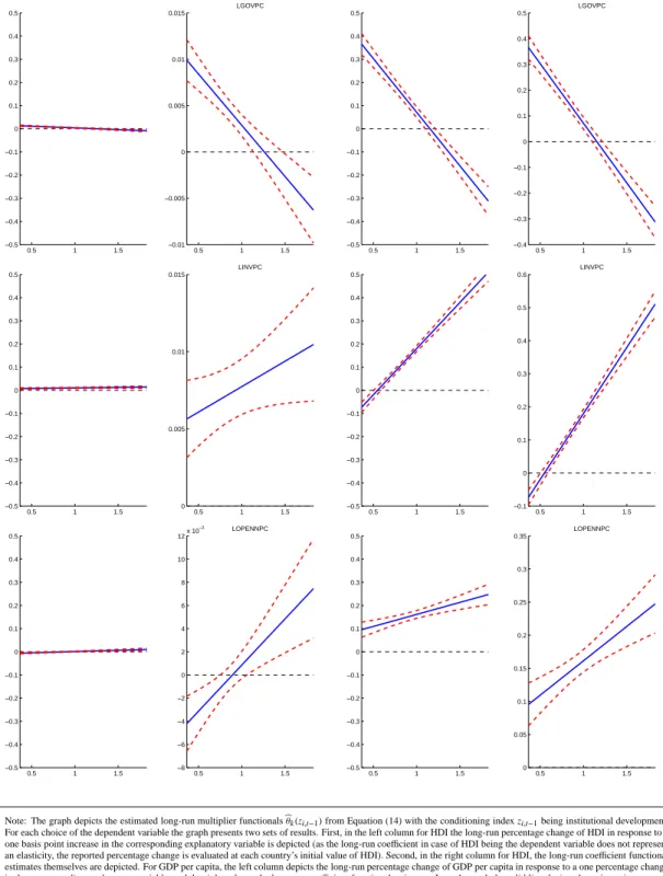
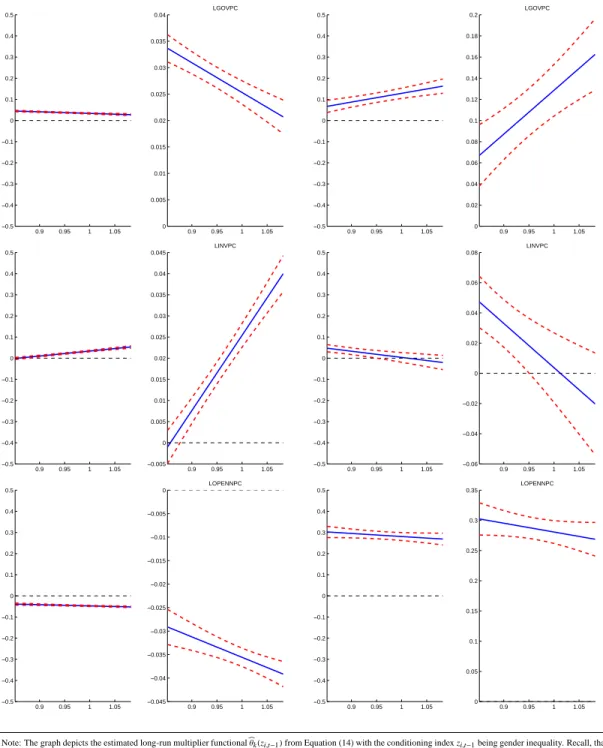
Concerning the estimated long-run coefficient functionals for the state-dependent panel
model in Equation (14) several observations stand out, as displayed in Figures 9 to 11. First, the figures, most strongly for GDP, but on a diminished scale also for HDI,
indi-cate strong state dependence of the development effects of economic policy changes, as
the estimated long-run coefficient functionals exhibit sizeable variation across different
cost of (erroneously) imposing cross-country homogeneity of the long-run development
effects of changes in economic policy. Let us turn second to specific policy variables and
conditioning state indices. Considering among the latter first institutional development,
the sign of the long-run effects of a fiscal (government consumption) stimulus varies for
both HDI and GDP across different levels of institutional quality. For countries with low
institutional quality, government consumption stimuli positively affect long-run HDI and
GDP, but for countries with high institutional quality, the long-run development effects
are negative, as for the Barro regression model. The scope of fiscal policy in the form of government consumption is much more limited for countries in which institutions are highly developed already. Strong institutional development, on the other hand, increases
the long-run development effects of both investment in physical capital and of trade
glob-alization, both for HDI and GDP, but again the stronger effects materializing for GDP.
Taken together, the fiscal (government consumption) stimulus and physical capital
invest-ment effects suggest that while government consumption expenditure in countries with
strong institutional development is not a suitable vehicle for long-run growth, a diff
er-ent assessmer-ent may hold for governmer-ent investmer-ent expenditure. With respect to gender
inequality, state variation of HDI development effects of economic policy changes is
actu-ally more pronounced across different stages of gender (in-)equality than across different
stages of institutional development. The strongest variation is observed for the long-run
HDI effects of changes in investment in physical capital, with these being about half a
percentage point higher in countries exhibiting (relative) success at moving towards
gen-der equality. The scale with which variations in gengen-der inequality affect long-run GDP
development is small when compared with the corresponding scale for institutional devel-opment. Also, as indicated by the standard error bands in Figure 10, there is uncertainty
regarding how the long-run GDP effects of physical capital investment vary across stages
environment, while the scale of state variation of the policy effects is large for GDP and
relatively large for HDI, the individual policy effect variations seem at best difficult to
rationalize. Why, for example, would the long-run increase of GDP per capita be about one whole percentage point larger in an environment in which the mix of religious af-filiations is slightly more growth conducive? From our perspective, the magnitude with
which the development effects of macroeconomic policies vary across different religious
environments make yet more transparent than for the Barro regressions that the religious
affiliation variables proxy for other societal characteristics, possibly including social trust,
and thus should not be taken at face value. For the remainder of this paper, therefore, we do not further pursue models that contain the religious environment index.
Exploiting the rich dynamic structure of our state-dependent panel model, we next com-pute dynamic multipliers depicting the full adjustment paths of HDI and of GDP per capita in response to a permanent ten percentage points increase in one of the economic policy variables. We compare the dynamic multipliers obtained from our state-dependent
dynamic panel model with the time path of the effect of the corresponding change in the
economic policy variables in period t = 0 obtained from the Barro regression
frame-work.23 To be specific about the computation of the dynamic multipliers, consider first
the Barro regression model in Equation (7),
T−1·(yiT −yi0)=β0+β1·yi0+γ#·xi+δ#· zi+ui.
Neglecting any transitional dynamics, a policy change in the --th x regressor implies a
23It is certainly sensible to argue that changes in, say, government consumption will in general also induce changes in physical capital investment and in international trade. However, as here we wish to emphasize the comparison between intertemporal adjustments as conventionally computed for the Barro regression model and those implied by our state-dependent panel model, we stick to computing orthogonal dynamic multipliers.
change in the long-run level of the dependent variable given by
*y-iT −yiT = T ·γ-·(*xi-−xi-), (15)
where *xi- denotes the value of the --th regressor after the policy change, and*y-iT the
corresponding new long-run level of yi. In case the dependent variable is HDI,*y-iT −
yiT reflects the level change of HDI relative to its baseline level after all adjustment has
taken place. In case the dependent variable is the logarithm of GDP per capita,*y
-iT −yiT
reflects the percentage change of GDP per capita relative to its baseline level after all
adjustment has taken place.24 Recall that in the Barro regression model the x variables
are measured as shares of GDP, while the x variables in the state-dependent panel data model are measured as per capita quantities. In order to work with comparable shocks
in the two models, for each country we calculate the increase in the share of x- in GDP
implied by a ten percent increase in x- in the state-dependent panel model, and use the
implied change in the share of x- in GDP as the shock to the Barro regression model.
Turning now to transitional dynamics, as follows from Appendix C.1, the transition path leading to the new long-run level of the dependent variable in the Barro regression model is given by
yit−yi0= (1−e−λt)·(*y-iT −yi0), (16)
with λ = −log(1+Tβ1)/T . For the calculation of the dynamic multipliers in the
state-dependent panel model, see Appendix D. The dynamic multipliers in Figure 13 display for all 84 countries in our sample the percentage change of HDI and of GDP per capita in response to a ten percentage points increase in one of the economic policy variables. To structure the large number of multipliers we compute, we decided to assign countries to one of three cross-country clusters, based on their observed average values of the
tioning state indices institutional development and gender inequality, and with the clusters constructed to create relatively homogenous country groupings according to the two state indices institutional development and gender inequality. We assign each country to one of these clusters: Cluster 1 containing all countries scoring well below average on gen-der inequality and at most average on institutional development; Cluster 2 containing all countries scoring in the extended medium range of values for institutional development and close to average or better on gender inequality; and Cluster 3 finally containing all countries scoring at least in the 80% percentile on institutional development - all these countries happen to have an average or higher score on gender inequality. See Figure 12 for a graphical illustration that these three clusters naturally emerge when considering the two state indices institutional development and gender inequality, and Table 7 for a listing of the countries within these three clusters. Each dynamic multiplier trajectory in Figure 13 corresponds to the average trajectory across the conditioning state indices institutional development and gender inequality: For each of these two indices, we trace
the in-sample effects of a period t = 0 (ten percent) increase of the x variable in
ques-tion if the state index had evolved as it actually did in sample.25 The Barro regression
based multipliers are, of course, state invariant and thus do not involve averaging across state indices. The left column in Figures 13 and 14 depicts the dynamic multipliers for all three clusters and all three economic policy variables under HDI being the dependent variable, and the right column depicts the dynamic multipliers under the logarithm of GDP per capita being the dependent variable. In each panel, the solid lines depict dy-namic multipliers obtained from the state-dependent panel model in Equation (14), and the starred lines depict the dynamic multipliers implied by the Barro regression model as given by Equation (16). Figure 13 depicts for the state-dependent panel model the
dy-25As the dynamic multipliers for our dynamic panel model are state dependent, there are other possibili-ties to compute dynamic multipliers, including integrating out the state dependence. See Koop, Pesaran and Potter (1996) for a general discussion in the time-series context.
namic multipliers for each country within a given cluster, whereas Figure 14 displays the averages of these dynamic multipliers across countries in a given cluster. Finally in Figure
14, the dash-dot line depicts the long-run effects as implied by the state-dependent panel
model. Several observations stand out upon inspection of Figures 13 and 14. First, there
is considerable heterogeneity across clusters in both the short- and the long-run effects of
the policy changes on both HDI and GDP per capita as implied by the state-dependent panel model. As just one example, while for countries in Cluster 3 GDP per capita grows
strongly after an increase in investment in physical capital, the effects of such a
stim-ulus are concentrated around zero for countries in Cluster 1. This heterogeneity of the dynamic multipliers in part reflects, of course, the state dependence of the long-run
co-efficient functionals discussed earlier in this section. It also reflects the country-specific
short-run dynamics inherent in our state-dependent panel model. The latter two sources of cross-country heterogeneity are also prominently present in the dynamic multipliers
reflecting the GDP effects of a fiscal (government consumption) stimulus: While the
av-erage long-run effects after a modest initial GDP gain are negative for Cluster 3, they
are positive for Clusters 1 and 2, though for these clusters also the short-run effects are
larger in magnitude than the long-run effects. Even in countries with limited institutional
development, therefore, the development scope of fiscal policy (in the form of
govern-ment consumption stimuli) is limited. Second, the policy effects on HDI implied by the
state-dependent panel model generally tend to be quantitatively, but in some instances
also qualitatively different from those on GDP per capita. For example, while an increase
in trade openness leads to an accumulating gain in GDP per capita across all clusters, the
same stimulus across all clusters negatively affects HDI. The dynamic multipliers
gener-ally make clear that the range of macroeconomic policies we consider impact HDI on a scale often about one tenth of that for the GDP impacts, both in the short and in the long
panel model are generally different from the corresponding effects in the Barro regression
model, not least because the Barro model implies homogenous effects across all
coun-tries and features linear adjustment processes. Only for specific cases are the multiplier
effects implied by the Barro regression model similar to the multiplier effects implied by
the state-dependent panel model. In general, even if one is interested in average effects
across certain societal characteristics, these cannot be well measured by a model neglect-ing prevailneglect-ing key heterogeneities.
Tables 8 and 9 focus on the long-horizon effects of the various economic policy changes
depicted in Figures 13 and 14, with Table 8 providing the development effects after 20
years, and Table 9 providing these effects in the steady state.26 The two tables highlight
some commonalities in the long-horizon development effects of changes in our three
eco-nomic policy variables. Stimuli in investment in physical capital across all three country
clusters and for both HDI and GDP have positive long-horizon effects - though the GDP
effects are significantly larger than those for HDI. For both HDI and GDP these effects
appear noticeably smaller, though, than suggested by the Barro regression model. For fiscal (government consumption) stimuli, as noted earlier, state conditioning plays a
par-ticulary pronounced role, in that for both HDI and GDP the long-horizon effects diminish
with advances in institutional development (and for HDI also with advances in gender
inequality) - for the GDP effects, these even turn negative, as also noted earlier. The
Barro regression model, though, seems to overstate the extent to which government
con-sumption stimuli may have detrimental long-term development effects. Last in terms of
commonalities of long-horizon effects, it is notable that across all three of our country
clusters the long-horizon effect of increased international trade are negative for HDI, and
(sizeably) positive for GDP.
26Table 9 also lists the steady state effects implied by the Barro regression models that were not plotted in Figures 13 and 14.
Let us finally discuss the relation between our findings in this section and those in Section 2. In Section 2, we had found evidence (see in particular Figures 1, 3 and 5) that HDI would exhibit unconditional convergence features not present in GDP. In this section, we found evidence that countries’ long-run development paths are state dependent, and that the conditional convergence process for HDI tends to be much more drawn out than that for GDP. Table 10 indicates a likely source for this apparent discrepancy of findings: At least for Africa and Asia, but to a weaker degree also for the OECD countries, there is (panel unit root test based) evidence that HDI is a unit root process; also, GDP appears to be a unit root process across all country groupings. While the (popular) methodology em-ployed in Section 2 is not valid in the presence of a unit root (bounded second moments then do not exist; a regression of the level of a variable on its growth rate is unbalanced and yields inconsistent parameter estimates), our state-dependent panel model is appli-cable even in the presence of unit roots. The latter model’s implications that both HDI and GDP converge conditionally to state-dependent development paths, with HDI adjust-ment significantly more drawn out than GDP adjustadjust-ment therefore need to be taken at face value. In Section 2, we had also found evidence that long-run levels development of HDI is quite closely aligned with that for GDP, but that such close alignment is not present in growth rates, even at a 35 years horizon. These findings are consistent with the empir-ical evidence accumulated in this section: While HDI and GDP may feature a common
stochastic trend, some core economic policies have notably different effects on HDI vs.
GDP growth even at extended horizons. It remains a question that is beyond the scope of this paper, though, to characterize the key factors underlying a common stochastic trend in HDI and GDP.
5
Conclusion
In this paper, we have applied a novel dynamic panel data model with state-dependent
coefficients to study the effects of a set of macroeconomic policies - investment in
phys-ical capital, government consumption and trade openness - on the development of HDI and GDP per capita. In contrast to the Barro regression model framework, the panel data model we apply does not require to a priori impose a decomposition of the data into short- and long-run dynamics, is able to account for potential endogeneity of the policy variables, allows for a high degree of cross-country heterogeneity in the development pro-cess, and is able to assess the quantitative role of countries’ persistent characteristics such as institutional quality, gender ()equality and religious environment. Among the key in-sights that have emerged from our analysis are: First, HDI development on various counts
differs notably from that of GDP. While both HDI and GDP exhibit conditional (though
not unconditional) cross-country convergence properties, the HDI adjustment process is slower than that for GDP. Realizing gains in HDI development requires more patience than in the case for GDP development policies. Also, macroeconomic policies such as international trade integration, stimulation of investment in physical capital and govern-ment consumption stimuli that may spur GDP developgovern-ment relatively notably will have
less pronounced effects for HDI. HDI development policies should look beyond the realm
of GDP development policies. Second, there are sizeable and important heterogeneities
in the development effects of macroeconomic policies across countries. Cross-country
differences in social norms and institutions may translate into differences in both the
tran-sitional dynamics and the long-run effects implied by economic policy changes. Our
findings in this regard underline the fallacy of “one size fits all” recipes, and highlight the importance of observing local conditions for the formulation of development strategies. One key example of this is that fiscal stimuli in the form of government consumption
posi-tively affect GDP in countries with low institutional quality, but negatively affect long-run GDP in countries with high institutional quality. The range of economic policies and
so-cietal characteristics rendering the development effects of changes in such policies state
dependent we have considered in this paper is rather limited. This is primarily due to data limitations that can hinder estimation of the state-dependent panel model even when a corresponding Barro regression model can be estimated. Much work on data measure-ment thus remains, and some of our other current work (see Binder and Georgiadis, 2010) is making start to remedy such limitations.
References
[1] Acemoglu, D., S. Johnson and J.A. Robinson (2001) “The Colonial Origins of Comparative Development: An Empirical Investigation,” American Economic Review, 91, 1369-1401. [2] Acemoglu, D., S. Johnson and J.A. Robinson (2005) “Institutions as the Fundamental Cause
of Long-Run Growth,” in P. Aghion and S. Durlauf (Eds.): Handbook of Economic Growth, Elsevier Science, 385-472.
[3] Barro, R.J. (1991), “Economic Growth in a Cross Section of Countries,” Quarterly Journal of Economics, 106, 407-443.
[4] Barro, R.J. and X. Sala-i-Martin. (2004), “Economic Growth,” MIT Press.
[5] Barro, R.J. and R. McCleary (2003), “Religion and Economic Growth,” NBER Working Papers, 9682.
[6] Binder, M. and M.H. Pesaran (1999), “Stochastic Growth Models and Their Econometric Implications,” Journal of Economic Growth, 4, 139-183.
[7] Binder, M. and C.J. Offermanns (2007), “International Investment Positions and Exchange
Rate Dynamics: A Dynamic Panel Analysis,” Center for Financial Studies Working Paper
No. 2007/23.
[8] Binder, M. and G. Georgiadis (2010), “Institutional and Financial Market Development of Nations: New Measures for a Large Panel,” Mimeo, Goethe University Frankfurt.
[9] Binder, M., G. Georgiadis and S. Sharma (2010), “Growth Effects of Financial
Globaliza-tion,” Mimeo, Goethe University Frankfurt.
[10] Brandolini, A. (2007), “On Applying Synthetic Indices of Multidimensional Well-Being: Health and Income Inequalities in Selected EU Countries,” Bank of Italy Economic Working Papers No. 668.
[11] Decancq, K. and M.A. Lugo (2008), “Setting Weights in Multidimensional Indices of Well-Being and Deprivation,” OPHI Working Paper No. 18.
[12] Evans, P. (1996), “Using Cross-Country Variances to Evaluate Growth Theories,” Journal of Economic Dynamics and Control, 20, 1027-1049.
[13] Freedomhouse (2009), “Freedom in the World 2009,” Freedom House, Inc., Washington, D.C.
[14] Gray Molina, G. and M. Purser (2010), “Human Development Trends since 1970: A Social
Convergence Story,” HDRO Working Paper, 01/2010.
[15] Hauk, W.R. and R. Wacziarg (2009), “A Monte Carlo Study of Growth Regressions,” Journal of Economic Growth, 14, 103-147.
[16] Heston, A., R. Summers and B. Aten (2009), “Penn World Table Version 6.3,” Center for International Comparisons of Production, Income and Prices at the University of Pennsylva-nia.
[17] Im, K.S., M.H. Pesaran and Y. Shin (2003), “Testing for Unit Roots in Heterogenous Panels,” Journal of Econometrics, 115, 53-74.
[18] Islam, N. (1995), “Growth Empirics: A Panel Data Approach,” Quarterly Journal of Eco-nomics, 110, 1127-1170.