Exact methods for nonlinear combinatorial optimization

for

Nonlinear Combinatorial Optimization

Dissertation

zur

Erlangung des Grades

eines

Doktors der Naturwissenschaften

Der Fakult¨

at f¨

ur Mathematik

der Technischen Universit¨

at Dortmund

vorgelegt von

Dipl.-Math.

Frank Baumann

aus Stolberg (Rhld.)

der Naturwissenschaften genehmigt.

Promotionsausschuss:

Vorsitzender: Prof. Dr. F. Kalhoff Erster Gutachter: Prof. Dr. C. Buchheim Zweiter Gutachter: Prof. Dr. P. Mutzel Dritter Pr¨ufer: Prof. Dr. C. Meyer

Tag der Einreichung: 22. April 2014 Tag der Disputation: 27. August 2014

We consider combinatorial optimization problems with nonlinear objective func-tions. Solution approaches for this class of problems proposed so far are either highly problem-specific or they apply generic algorithms for constrained nonlinear optimization, which often does not yield satisfactory results in practice.

Our aim is to develop, implement and experimentally evaluate exact algorithms that address the nonlinearity of the objective function and at the same time ex-ploit the underlying combinatorial structure of the problem. To this end we follow two approaches. The first combines good polyhedral descriptions of the objective function and the feasible set in a branch and cut-algorithm. The second approach is based on Lagrangean decomposition. By decomposing the original problem into an unconstrained nonlinear problem and a linear combinatorial problem, we are able to compute strong dual bounds for the optimal value. The computation of lower bounds is then embedded into a branch and bound-algorithm. For many applications there already exist efficient algorithms for the combinatorial sub-problem, thus an important aspect of this thesis is the study of the corresponding unconstrained nonlinear subproblems.

Both approaches have the advantage that they can easily be adapted to a wide range of nonlinear combinatorial problems. We devise both polyhedral and decom-position-based algorithms for submodular applications from wireless network de-sign and portfolio optimization and evaluate their performance experimentally. Exploiting the equivalence between unconstrained binary quadratic optimiza-tion and the maximum cut problem gives rise to a branch and cut-algorithm for quadratic combinatorial problems which we use to compute optimal layouts of tanglegrams, an application from computational biology. Additionally we study the effect of quadratic reformulation of linear constraints, both theoretically and experimentally. The last class of nonlinear combinatorial problems we consider are two-scenario problems. Here we propose a new technique to compute lower bounds in the unconstrained subproblem of the decomposition. Our computa-tional study of the two-scenario minimum spanning tree problem shows that the new Lagrangean decomposition-based algorithm is able to solve significantly larger instances than the standard linearization approach.

Diese Arbeit besch¨aftigt sich mit der exakten L¨osung kombinatorischer Opti-mierungsprobleme mit nichtlinearen Zielfunktionen. Bisher werden f¨ur diese Art von Problemen meist entweder hochgradig problemspezifische Algorithmen ent-wickelt, oder es kommen L¨oser f¨ur allgemeine beschr¨ankte nichtlineare Probleme zum Einsatz, was in der Praxis aber oft nicht zu befriedigenden Ergebnissen f¨uhrt. Ziel dieser Arbeit ist daher die Entwicklung, Implementierung und experimentelle Evaluation exakter Algorithmen, die sowohl die Nichtlinearit¨at der Zielfunktion als auch die zugrunde liegende kombinatorische Struktur des Problems ausnutzen. Dazu verfolgen wir zwei Ans¨atze. Im ersten werden gute polyedrische Beschrei-bungen der Zielfunktion und der kombinatorischen Struktur in einem Branch-and-Cut Algorithmus kombiniert. Der zweite basiert auf Lagrange-Dekomposition. Hier wird das Ausgangsproblem in ein unbeschr¨anktes nichtlineares und ein linea-res kombinatorisches Problem zerlegt. Das erlaubt die Berechnung starker dua-ler Schranken in einem Branch-and-Bound Algorithmus. F¨ur viele Anwendungen sind bereits effiziente Verfahren zur L¨osung des kombinatorischen Teilproblems bekannt. Ein wichtiger Beitrag dieser Arbeit besteht daher in der Untersuchung der auftretenden unbeschr¨ankten nichtlinearen Teilprobleme.

Beide Ans¨atze haben den Vorteil, dass sie sich ohne großen Aufwand auf eine Vielzahl nichtlinearer kombinatorischer Problemstellungen anwenden lassen. Wir betrachten drei Klassen von nichtlinearen kombinatorischen Optimierungspro-blemen. Im Falle einer submodularen Zielfunktion sind beide oben beschriebenen Ans¨atze anwendbar. Wir stellen exakte Algorithmen f¨ur Anwendungen aus dem Bereich der mobilen Daten¨ubertragung und der Portfoliooptimierung vor und vergleichen sie experimentell mit Standardverfahren. Bei quadratischen Zielfunk-tionen ergibt sich aus der ¨Aquivalenz von unbeschr¨ankter bin¨arer quadratischer Optimierung und der Berechnung eines maximalen Schnittes in einem Graphen eine gute polyedrische Charakterisierung der Zielfunktion, die in einem Branch-and-Cut Algorithmus verwendet werden kann. Damit lassen sich Tanglegrams berechnen, die u.a. in der Bioinformatik Anwendung finden. Desweiteren unter-suchen wir die Auswirkungen, die verschiedene quadratische Reformulierungen von linearen Nebenbedingungen auf die G¨ute der dualen Schranken im Branch-and-Cut Algorithmus haben. Als letzte Klasse werden Zwei-Szenario-Probleme behandelt. Wir stellen eine neue Technik zur Berechnung unterer Schranken f¨ur das unbeschr¨ankte Teilproblem in der Lagrange-Dekomposition vor. Eine experi-mentelle Studie anhand des minimalen Spannbaumproblems mit zwei Szenarien zeigt, dass sich mit dem neuen dekompositionsbasierten Algorithmus deutlich gr¨oßere Instanzen l¨osen lassen als mit dem auf ganzzahliger Programmierung basierenden Standardansatz.

Teilergebnisse der vorliegenden Arbeit sind bereits in den folgenden Publikationen ver¨offentlicht worden:

Frank Baumann, Christoph Buchheim, and Anna Ilyina. Lagrangean decompo-sition for mean-variance combinatorial optimization. Lecture Notes in Computer Science, 2014. ISCO 2014 – International Symposium on Combinatorial Opti-mization, to appear.

Frank Baumann, Sebastian Berckey, and Christoph Buchheim. Exact algorithms for combinatorial optimization problems with submodular objective functions. In Michael J¨unger and Gerhard Reinelt, editors,Facets of Combinatorial Opti-mization, pages 271–294. Springer Berlin Heidelberg, 2013.

Frank Baumann and Christoph Buchheim. Submodular formulations for range assignment problems. Electronic Notes in Discrete Mathematics, 36(0):239–246, 2010. ISCO 2010 – International Symposium on Combinatorial Optimization. Frank Baumann, Christoph Buchheim, and Frauke Liers. Exact bipartite cross-ing minimization under tree constraints. In Paola Festa, editor, Experimental Algorithms, volume 6049 ofLecture Notes in Computer Science, pages 118–128. Springer Berlin Heidelberg, 2010.

Acknowledgements

I would like to express my thanks to everyone who supported me throughout my work on this thesis. I am particularly indebted to my supervisor Prof. Christoph Buchheim for his scientific guidance and the pleasant and stimulating working atmosphere he created in his group.

I am very grateful to Frauke Liers for introducing me to tanglegrams and the subsequent collaboration, which led to Chapter 5 of this thesis.

Many thanks go to my colleagues in Cologne, Dortmund and elsewhere for the many constructive and helpful discussions, especially to Viktor Bindewald, Anja Fischer, Anna Ilyina, Laura Klein, Jannis Kurtz, Sara Mattia, Dennis Michaels, Maribel Montenegro, Marianna De Santis, Emiliano Traversi and Long Trieu, and to Sabine Willrich for perfectly taking care of all administrative issues.

Part of my work was funded by the DFG as part of the project Simple and Fast Implementation of Exact Optimization Algorithms with SCILin thePriority Pro-gramme 1307 Algorithm Engineering and the project Lenkung des G¨uterflusses in durch Gateways gekoppelten Logistik-Service-Netzwerken mittels quadratischer Optimierung, which is gratefully acknowledged.

Finally, I would like to thank my family for their invaluable support and encour-agement.

Introduction 1 Outline 3

I

Methods

7

1.3 Branch and Bound . . . 16

1.3.1 LP-Based Branch and Bound . . . 18

1.3.2 Lagrangean Decomposition-Based Branch and Bound . . . 18

1.3.3 SDP-Based Branch and Bound . . . 19

1.3.4 Enumeration Strategies . . . 21

1.4 Branch and Cut . . . 21

2 Binary Quadratic Optimization 23 2.1 Standard Linearization . . . 23

2.2 Unconstrained Binary Quadratic Optimization . . . 25

2.2.1 Odd Cycle Inequalities . . . 27

2.2.2 More Cutting Planes . . . 31

2.3 Quadratic Reformulation . . . 33

2.3.1 SQK2 . . . 34

2.3.2 SQK3 . . . 37

3 Submodular Combinatorial Optimization 45

3.1 Submodularity . . . 46

3.2 Constructing Submodular Functions . . . 47

3.3 Polyhedral Study . . . 52

3.4 A Branch and Cut Approach . . . 58

3.4.1 Cutting Planes . . . 58

3.4.2 Primal Bounds . . . 58

3.5 A Lagrangean Decomposition Approach . . . 59

3.5.1 Bounds . . . 59

3.5.2 Branch and Bound . . . 61

3.6 Final Remarks . . . 62

4 Two-Scenario Optimization 65 4.1 Unconstrained Two-Scenario Optimization . . . 65

4.1.1 Complexity . . . 66

4.1.2 Transformation to Fractional Knapsack Problems . . . 67

4.1.3 An Exact Algorithm . . . 69

4.2 Combinatorial Two-Scenario Optimization . . . 70

4.2.1 Lower Bounds . . . 71

4.2.2 An Exact Algorithm . . . 72

4.3 Two-Scenario Min-Max Regret Problems . . . 73

II

Applications

75

5.2 An Exact Model for General Tanglegrams . . . 82

5.2.1 Bipartite Crossing Minimization . . . 83

5.2.2 Modeling Tanglegrams . . . 84

5.2.3 Binary Case . . . 85

6 Combinatorial Quadratic Optimization 91

6.1 Quadratic Minimum Spanning Tree . . . 91

6.1.1 Quadratic Reformulation . . . 93

6.1.2 Computational Results . . . 93

6.2 Quadratic Matching . . . 97

6.2.1 Computational Results . . . 99

7 Range Assignment Problems 105 7.1 The Standard Model . . . 109

7.2 New Mixed-Integer Models . . . 109

7.3 Polyhedral Relations . . . 110 7.4 Computational Results . . . 111 7.4.1 Symmetric Connectivity . . . 111 7.4.2 Multicast . . . 115 7.4.3 Broadcast . . . 116 7.5 Final Remarks . . . 116

8 Mean Risk Optimization 119 8.1 Computational Results . . . 125

8.2 Final Remarks . . . 131

9 Two-Scenario Optimization 133 9.1 Unconstrained Two-Scenario Optimization . . . 133

9.2 Two-Scenario Minimum Spanning Tree . . . 136

III

Nonlinear Optimization with SCIL

143

Summary and Outlook 149

Combinatorial optimization deals with finding an optimal solution for problems with finite sets of feasible solutions. Often these problems are stated in graph-theoretic terms and solution methods include techniques from algorithm theory as well as polyhedral combinatorics and linear programming. For many applications that can be modeled as combinatorial optimization problems efficient algorithms are known, for others the best known algorithms have an exponential theoretical complexity.

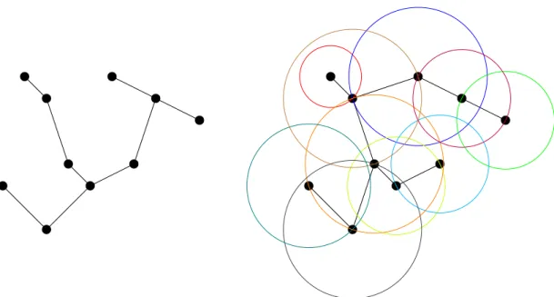
Consider for example a task frequently encountered in the design of networks, e.g. for telecommunication. You are given a set of nodes with fixed coordinates in the plane and your job is to decide between which pairs of nodes connections are established by laying subterranean cables. In the end the network must be connected, i.e. it must be possible to reach any given node from any given starting point via the chosen links (see Figure 1 (left)). Establishing a connection is asso-ciated with costs, for example proportional to the length of the link, and the total cost of a network is given by the sum of the costs of the established connections. Which links do you choose such that the total cost is minimal? This problem is known as the minimum spanning tree problem. It is well-studied and several efficient and surprisingly simple solution algorithms are known; the earliest was proposed by Boruvka [17] in 1926.

Now imagine the task is slightly different. Nodes are not linked by laying cables in the ground but wirelessly. A connection between two nodes a and b can only be established if the signal transmitted from a is strong enough to reach b and vice versa. The goal as before is a connected network, but now your task is to choose which connections to make and to set appropriate transmission powers for the individual nodes (see Figure 1 (right)). The cost of the network in this case is determined by its total transmission power. This variant of the minimum spanning tree problem is called range assignment problem. Although both prob-lems seem to be very similar, the second is much harder to solve than the first. In fact, no polynomial-time algorithm for the range assignment problem is known and only very small instances can be solved in practice.

Another example of an application where a slight variation in the problem state-ment increases its difficulty significantly is the knapsack problem. You are given

Figure 1: Optimal wired (left) and wireless (right) networks for the same set of nodes. The colored circles on the right indicate the transmission ranges of the nodes in the wireless network.

a set of items characterized by a weight and a profit and a knapsack with limited capacity. An optimal solution of the knapsack problem is a subset of the items that fits into the knapsack and gives maximum profit. The knapsack problem is closely related to a problem from portfolio theory, the so-called risk-averse cap-ital budgeting problem. Here an investor has to choose from a set of possible investments. His budget is limited and in contrast to the knapsack problem the expected profits are not known exactly in advance. Instead they are characterized by an expected return value and a variance. The knapsack problem can be solved in pseudo-polynomial time. The exact complexity of the risk-averse capital bud-geting problem is unknown, but in practice it is much harder than the knapsack problem.

In both examples given above the two problems have the same combinatorial structure, the increase in the complexity is caused by the change in the objective function. In the minimum spanning tree problem and the knapsack problem it is linear, whereas in the range assignment problem and the risk-averse capital budgeting problem it is nonlinear. Nonlinear combinatorial optimization problems are commonly solved either with highly application-specific algorithms or with generic solvers for constrained nonlinear optimization. The first approach has the advantage that the underlying combinatorial structure is exploited, but the resulting algorithms are not easily adaptable to other nonlinear applications. The second approach is more versatile but often focuses on the nonlinear aspect of the problem and disregards the combinatorial structure.

In this thesis we study exact solution techniques for nonlinear combinatorial optimization problems that address the nonlinearity of the objective function and at the same time exploit the underlying combinatorial structure of the problem. The main idea of our approach is to treat the nonlinear objective function and the part of the problem formulation that models the set of feasible solutions independently. This allows us to combine solution techniques from unconstrained binary nonlinear optimization and linear combinatorial optimization to compute dual bounds for the original problem. Embedding the computation of dual bounds in a branch and bound-algorithm yields an algorithmic framework that can be easily customized to solve a wide range of nonlinear combinatorial applications. For this approach to give good results in practice it is essential that the occurring subproblems can be solved to optimality quickly, or, when this is not possible, strong dual bounds can be computed efficiently. As exemplified above, in many cases the linear variant of an application is well-studied and we can use existing algorithms and polyhedral characterizations to solve the combinatorial subprob-lem. In contrast, the corresponding unconstrained nonlinear subproblems have often not been studied intensively so far. Therefore, we investigate several classes of nonlinear objective functions and propose efficient algorithms for some special cases.

Outline

This thesis is divided into three parts. Part I deals with general techniques for the exact solution of three classes of nonlinear combinatorial optimization prob-lems. We start by giving the necessary basic definitions and notations used in the following chapters. In Chapter 2 we discuss the polyhedral approach to bi-nary quadratic optimization that exploits the equivalence between unconstrained binary quadratic optimization and the MaxCut problem [28] and study the effec-tiveness of quadratic reformulation of linear constraints in this context. We pro-pose a reformulation technique for assignment constraints that leads to stronger relaxations without increasing the number of variables in the problem formula-tion.

In Chapter 3 we study combinatorial optimization problems with submodular ob-jective functions. We propose two exact algorithms. The first is a branch and cut-algorithm based on a polyhedral description of the convex hull of feasible points of the unrestricted problem by Edmonds [36]. The second is again a branch and bound-algorithm, but here lower bounds are computed by applying Lagrangean decomposition to the original formulation. This yields two subproblems, an unre-stricted submodular minimization problem and a linear combinatorial problem. Chapter 4 deals with two-scenario optimization. We first study the problem of

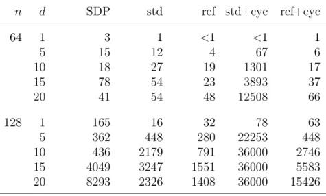
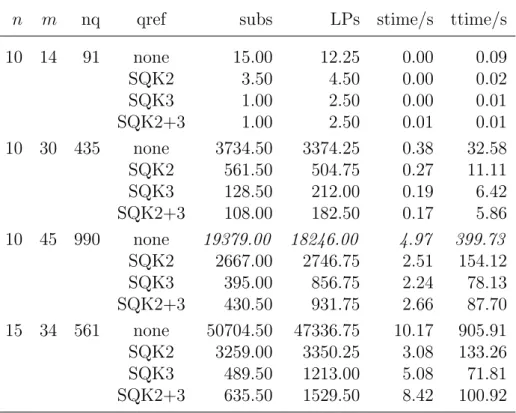
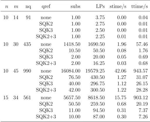
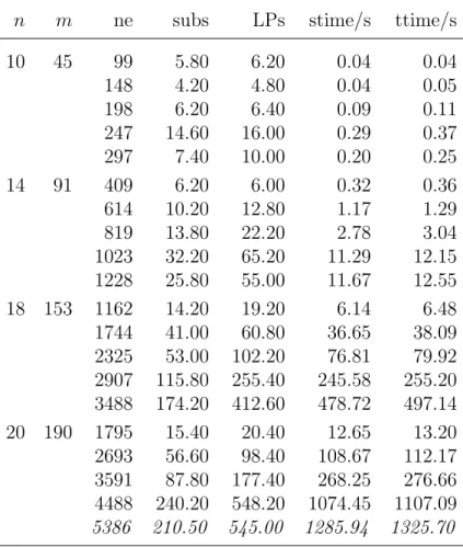
minimizing the maximum of two linear functions over bounded integer variables and propose a bounding technique that applies a transformation to two fractional knapsack problems. This approach leads to an exact branch and bound-algorithm for unconstrained two-scenario optimization problems. In the presence of addi-tional combinatorial constraints this approach can still be used to compute lower bounds. To this end we again apply Lagrangean decomposition, as in Chapter 3. This yields an exact branch and bound-algorithm that for certain classes of com-binatorial two-scenario problems does not require solving linear programs. In Part II we use the general techniques proposed in the first part to devise exact algorithms for specific nonlinear applications. We start in Chapter 5 with computing optimal layouts of tanglegrams, which are for example used in compu-tational biology to visualize the co-evolution of two species. This problem can be modeled as a quadratic linear ordering problem with additional constraints. In an experimental study we solve random and realistic instances to evaluate the effect of MaxCut-separation and quadratic reformulation. The experimental study is continued in Chapter 6 on the quadratic variants of the minimum spanning tree problem and the perfect matching problem.

The range assignment and mean risk optimization problems studied in Chapters 7 and 8 are generalizations of classic combinatorial problems, where the objective function is submodular instead of linear. Range assignment problems occur in wireless network design, where the overall costs are not determined by the total lengths of the established links but by the transmission power needed to establish a given network topology [122], as illustrated above. Although such problems have been studied intensively in recent years, the algorithms proposed in the literature so far do not directly exploit the submodularity of the objective function [98]. We devise a fast algorithm for the minimization of the submodular subproblem in the Lagrangean decomposition approach and evaluate the performance of the two algorithms proposed in Chapter 3 experimentally for three network topologies. Mean risk optimization problems are used in finance to compute optimal in-vestment strategies [24]. They are commonly solved as second-order cone prob-lems [10]. We model the risk-averse capital budgeting problem, which served as our second example in the introduction, as a knapsack problem with a submod-ular objective function and compare the performance of the new approaches to the standard method.

In the last chapter of Part II we present an extensive experimental study of the algorithms for unconstrained and combinatorial two-scenario optimization presented in Chapter 4. For the combinatorial case we consider the two-scenario minimum spanning tree problem, which has applications in the design of robust telecommunication networks [77].

Part III gives a brief overview of the optimization library SCIL. For this thesis it was extended by the polyhedral methods for submodular and quadratic

optimiza-tion problems presented in Chapters 2 and 3 and used for the implementaoptimiza-tion of the branch and cut-algorithms in Part II.

We conclude this thesis with a summary of our results and a brief discussion of possible extensions and future work.

Methods

Preliminaries

In this chapter we first fix some notation and give basic definitions that will be used throughout the remaining chapters. Then we give the basic theoretical background for later chapters. Notations and definitions follow the text books by Nemhauser and Wolsey [100], Wolsey [123] and Korte and Vygen [76].

1.1

Basic Definitions

Sets Sets are denoted by capital letters. For sake of legibility we write A∪k

instead ofA∪ {k} for the union of a set A and a single elementk.

Graphs In the following, G = (V, E) denotes an undirected graph. V =

{1, . . . , n} is a finite set called the set of nodes and the set of edges E con-sists of two-element unordered subsets of V. An edge e = (u, v) ∈ E is said to connect nodes uand v and it isincident to both uand v. The nodesu an v are sometimes called the endpoints ofe. Two edges with a common node areadjacent

and an edge (u, u) that connectsuto itself is called aloop. Graphs without loops are calledsimple. In this thesis we will only consider simple graphs. Note that in our definition of graph two nodes are connected by at most one edge, i.e. they do not have multiple edges. If the graph is directed, we write G = (V, A). The arc set A consists of ordered pairs of nodes. The first node in the ordered pair defining an arc a is called the tail of a, the second the head of a. In a weighted graph – undirected or directed – each edge (arc) is assigned a weight by aweight function c: E −→ _Q (c: E −→ _Q). These graphs are denoted by G = (V, E, c) and G= (V, A, c), respectively.

For a setU ⊆V,E(U) = {(i, j)|(i, j)∈E, i∈U, j ∈U}is the set of edges with both endpoints inU. A subgraphG′ of a graphG consists of a subsetV′ ⊆V of the nodes of Gand a subset E′ ⊆E(V′) of the edges with both endpoints inV′.

G′ is called a spanning subgraph if V′ =V.

Paths A sequence of nodes (v0, . . . , vk),k∈Nof an undirected graph is called

awalk, if (vi, vi+1)∈E for alli∈ {0, . . . , k−1}. If each node occurs exactly once, the walk is called a path in G. A graph that contains a walk between each pair of nodes is called connected.

Walks and paths can also be expressed by a sequence of edges (e0, . . . , ek−1). By adding the edge ek = (vk, v0) we obtain a closed walk w. If (e0,· · · , ek−1) is a path containing at least two edges, w is called a cycle.

Trees A tree is a connected undirected graph without cycles. An arborescence

is an acyclic directed graph (DAG) in which all arcs point away from a specified root node. This is equivalent to the property that for each vertex v ∈ V \ {v}

there exists a directed path from r to v. In a Steiner arborescence only a subset

T ⊆V \ {v}, calledterminals, must be reachable via directed paths from the root node. These paths can include the Steiner nodes V \(T ∪ {r}).

Optimization problems and relaxations Given a function f: _Rn _−→

R

and a set A ⊆ _Rn_{, a general optimization problem (P) consists of finding a}

minimizer or maximizer off inA. In the following we limit ourselves to discussing minimization problems and write (P) as

min f(x)

s.t. x ∈ A⊆_Rn_,

or shorter as

min{f(x)|x∈A}.

The function f is called the objective function of (P) and A its set of feasible solutions or feasible region. If A = ∅, (P) is infeasible. If (P) is feasible, the minimizer of f in A is denoted by x⋆ and the value f(x⋆) is called the optimum value of (P). In a slight abuse of notation, we sometimes write

z = min{f(x)|x∈A}

to refer to the optimization problem and its optimum value z. Given a second optimization problem

min{g(x)|x∈B}, (Q)

(Q) is a relaxation of (P) if A⊆B and f(x)≥g(x) for each x∈A.

The objective function value of any feasible solution of (P) defines an upper or

primal bound on the optimum value of (P), while any optimum value of a relax-ation defines a lower or dual bound. For maximization problems upper bounds are dual bounds, while lower bounds are primal bounds.

In a combinatorial optimization problem the set of feasible solutions is finite. Combinatorial optimization problems are a special case of so-calledmixed-integer

programs (MIPs), where some or all of the variables are required to take only integer values. They are often used to model optimization problems on graphs. Say you want to compute a minimum-cost spanning tree in an undirected graph

G = (V, E, c). The first step is to associate each edge e ∈ E of the graph with a binary variable xe. Then the set of feasible solutions, in this case the set of

spanning trees in G, is modeled by a set of equations and inequalities in these variables. The result is abinary optimization problem. When we associate binary variables with elements of some set D, we often denote the sum of the variables associated withD as x(D) instead of 

i∈Dxi.

If the equations and inequalities used are linear and c is a linear function, the problem is called an integer linear program (ILP) and generally written as

min c⊤x

s.t. A1x = b1

A2x ≤ b2

x ∈ {0,1}n_.

Definition 1.1. For two optimization problems min f(x)

s.t. x ∈ X ⊆_Rn (1.1)

and

min g(y)

s.t. y ∈ Y ⊆_Rm (1.2)

denote by X⋆ _{⊆X and Y}⋆ _{⊆ Y the sets of optimal solutions of (1.1) and (1.2),}

respectively.

Problems (1.1) and (1.2) areequivalent, if

1. there exists a bijective function h: X⋆ −→Y⋆, i.e. for every y⋆ ∈Y⋆ there exists a unique x⋆ _∈X⋆ _{with y}⋆ _=h(x⋆_{), and}

2. g(h(x⋆)) = f(x⋆) for all x⋆ ∈X⋆, i.e. equivalent optimal solutions have the same objective value.

The two problems are calledisomorphic, if

1. there exists a bijective function h: X −→ Y, i.e. for every y ∈ Y there exists a unique x∈X with y =h(x), and

2. g(h(x)) = f(x) for all x ∈ X, i.e. equivalent feasible solutions have the same objective value.

Obviously, when two optimization problems are isomorphic, they are also equiv-alent.

Definition 1.2. Given a nonlinear optimization problem min f(x)

s.t. x ∈ X ⊆_Rn_, (P1) the problem

min g(y)

s.t. y ∈ Y ⊆_Rm (P2) is a linearization of (P1), if (P1) and (P2) are equivalent and (P2) is a linear optimization problem.

Polyhedra A polyhedron P in _Rn is a set of points that can be characterized by a finite number of linear inequalities: P = {x ∈ _Rn _{| Ax ≤ b}. A bounded}

polyhedron is called a polytope. Given a nonempty polyhedron P and a nonzero vector c∈_Rn _{for which δ:= max{c}⊤_{x|x∈P} is finite, the set{x∈}

Rn|c⊤x=

δ} is called a supporting hyperplane of P. A face of P is the intersection of P

with one of its supporting hyperplanes or P itself. Faces of maximal dimension are called facets, where the dimension of a set is defined as the dimension of the smallest affine space that contains the set.

A linear inequality a⊤x ≤ δ is called valid for P, if it holds for all x ∈ P. If additionally {x ∈ P | a⊤x = δ} is a facet of P, the inequality is called facet-defining.

Theconvex hull conv(X) of a setX is the set of all convex combinations of points in X, i.e. the set of all points ¯x that can be expressed as

¯ x= |X|  i=1 λixi

with appropriately chosen multipliers λ1, . . . , λ|X| ≥0 with|_iX₌₁|λi = 1.

Definition 1.3. Given a set of linear inequalitiesAx≤band binarity constraints on some of the variables, relax the binarity constraints to box constraints, such that 0 ≤x≤1. The set of points which are feasible for the resulting problem is called the polytope corresponding to Ax≤b.

1.2

Lagrangean Relaxation

Consider a mixed-integer linear optimization problem of the form min x≥0 c ⊤_x s.t. Ax ≤ a Bx ≤ b xi ∈ Z ∀i∈I , (P) withA∈_Rp×n_{,B ∈} Rq×n,c∈Rn, a∈Rp,b ∈Rq, andp, q, n ∈N+.I is a subset of the variable indices. It is assumed that the constraints are divided into two sets such that solving problem (P) without constraints Ax ≤a is significantly easier than solving the complete problem (P). The basic idea of Lagrangean relaxation is to treat the complicating constraints by moving them to the objective function. Violation of these constraints is penalized by so-calledLagrangean multipliers λ. The resulting problem, theLagrangean relaxation with respect to Ax≤aof (P), reads min x≥0 c ⊤ x+λ⊤(Ax−a) s.t. Bx ≤ b xi ∈ Z ∀i∈I , (LRλ)

with λ ∈ _Rp_≥0. For each feasible value of λ, the optimum value of (LRλ) gives a

dual bound of problem (P). The problem of determining values for λ that give the best possible dual bound z is called theLagrangean dual problem:

z= max λ∈_Rp_≥0minx≥0 c ⊤ x+λ⊤(Ax−a) s.t. Bx ≤ b xi ∈ Z ∀i∈I (D)

Denote by (P⋆) the following relaxation of (P): min x c ⊤ x s.t. Ax ≤ a x ∈ conv{x≥0|Bx≤b, xi ∈Z∀i∈I} (P⋆) The next theorem characterizes the relation between the relaxations (LRλ), (P⋆)

and the LP relaxation ¯P of (P).

Theorem 1.1 (Geoffrion [50]). Denote by v(·) the optimum solution value of a problem.

1. For all λ ≥0 (LRλ) is a relaxation of (P):

(P⋆_{) is at least as tight as the LP relaxation:}

F( ¯P)⊇F(P⋆)⊇F(P) and v( ¯P)≤v(P⋆)≤v(P)

2. The relaxation (P⋆_{) gives the same dual bound as the Lagrangean dual:}

z =v(P⋆)

If the optimal value of the relaxation (P Rλ) does not change when the integrality

conditions on the variables are dropped, (P Rλ) is said to have the integrality

property. In this case the value of the Lagrangean dual is the same as the value of the LP-relaxation ( ¯P).

By Theorem 1.1 the value of the Lagrangean dual is always as least as good as the value of the LP-relaxation, but it can be better if (P Rλ) does not have

the integrality property. This means that it is desirable to choose the constraints to be relaxed such that the resulting Lagrangean relaxation does not have the integrality property.

Theorem 1.2. Let( ¯P)be feasible and(P Rλ)have the integrality property. Then

(P⋆_{) is feasible and}

v( ¯P) = z .

An optimal solution of the Lagrangean relaxation LRλ in general is not optimal

for the original problem (P), unless it satisfies the following optimality conditions. Theorem 1.3 (Geoffrion [50]). Let x⋆ be an optimal solution of the Lagrangean relaxation (LRλ) for a given λ. x⋆ is optimal for (P) if

1. Ax≤a

2. λ⊤(Ax−a) = 0.

1.2.1

Lagrangean Decomposition

Lagrangean decomposition can be considered a Lagrangean relaxation with re-spect to a set of artificial constraints. Its aim is to decompose the problem into auxiliary problems that can be easily computed. Starting as before from the problem min x≥0 c ⊤_x s.t. Ax ≤ a Bx ≤ b xi ∈ Z ∀i∈I , (P)

we introduce new variables y ≥ 0 and artificial linking constraints and express the second set of constraints in the new variables:

min x≥0 c ⊤_x s.t. Ax ≤ a By ≤ b x = y xi ∈ Z ∀i∈I ,

Applying Lagrangean relaxation to the linking equations gives min x≥0 c ⊤_x+λ⊤_(x−y) s.t. Ay ≤ a Bx ≤ b xi ∈ Z ∀i∈I ,

Since the two sets of constraints are now independent of each other the problem decomposes into min x≥0 c ⊤_x+λ⊤_{x + min} y≥0 −λ ⊤_y s.t. Bx ≤ b s.t. Ay ≤ a xi ∈ Z ∀i∈I (LDλ)

Guignard and Kim [55] showed that the bound provided by the Lagrangean decomposition is at least as good as the bound obtained from the Lagrangean relaxation of one of the two sets of constraints.

Theorem 1.4. Let λ⋆ _{be an optimal multiplier for max}

λ≥0 v(LRλ), µ

⋆ _{= λ}⋆_{A and}

(x⋆_{, y}⋆_{) optimal for (LD}

µ⋆), i.e. optimal for

min x≥0{c ⊤ x+ (a−µ⋆)⊤x|Bx≤b, xi ∈Z ∀i∈I} and min y≥0{−µ ⋆⊤ y |Ay≤a}. Then 1. v(LDµ⋆)−v(LR_λ⋆) = (λ⋆)⊤(a−Ay⋆) 2. max µ∈_R v(LDµ)≥maxλ≥0 v(LRλ) The proof is straight forward.

Proof. Let λ⋆ _{be an optimal multiplier for max}

λ≥0 v(LRλ) and µ

⋆ _=A⊤_λ⋆_{. Choose}

(x⋆_{, y}⋆_{) such that it is an optimal solution of (LD}

µ⋆). Then v(LDµ⋆) = min x≥0{c ⊤ x+ (µ⋆)⊤x|Bx≤b, xi ∈Z ∀i∈I}+ min y≥0{(−µ ⋆₎⊤ y|Ay≤a} = min x≥0{c ⊤ x+ ((λ⋆)⊤A)x|Bx≤b, xi ∈Z ∀i∈I}+ min y≥0{((−λ ⋆ )⊤A)y |Ay≤a} =c⊤x⋆+ (λ⋆)⊤Ax⋆ + ((−λ⋆)⊤A)y⋆ ((x⋆_{, y}⋆_{) is optimal for (LD} µ⋆)) =c⊤x⋆+ (λ⋆)⊤A)x⋆ −(λ⋆)⊤a+ ((λ⋆)⊤a)−(λ⋆)⊤Ay =c⊤x⋆+ (λ⋆)⊤(Ax⋆ −a)+ (λ⋆)⊤(a−Ay⋆) =v(LRλ⋆) + (λ⋆)⊤(a−Ay⋆)

The last equality holds, because, by the choice of µas µ⋆ =A⊤λ⋆ the first part of (LDµ⋆) and (LR_λ⋆) differ only by a constant term in the objective function.

Since (x⋆_{, y}⋆_{) is optimal for (LD}

µ⋆),x⋆ is also optimal for (LR_λ⋆).

This proves the first part of the theorem. Since both λ⋆ and a−Ay⋆ are non-negative, also the second part follows.

Concluding the preliminaries, we will give a short description the branch and bound- and branch and cut-approaches for (mixed-)integer programs. These two techniques will be used throughout this thesis to compute optimal solutions of nonlinear optimization problems. We will limit the exposition in the following two sections to the basic concepts; details concerning the adaptation of the algorithms to specific problem types and applications will be discussed in later chapters. For a more detailed introduction to branch and bound- and branch and cut-algorithms, see [75] and [94]. Computational issues are discussed in [90].

1.3

Branch and Bound

Branch and bound is a technique to compute optimal solutions of optimization problems. Although it was originally proposed by Land and Doig [79] as an al-gorithm for MIPs, it is applicable whenever bounds on the optimal value of the optimization problem can be computed. As the name suggests, a branch and algorithm has two main components, a branching procedure and a bound-ing procedure. The boundbound-ing procedure optimizes an objective function over a given feasible region and the branching procedure decomposes a given feasible region into two or more smaller sets. The main idea of the branch and bound-algorithm is to break up the original problem into a series of smaller subproblems

which are easier to solve. The information obtained from the subproblems is then used to determine an optimum solution of the original problem. This approach is motivated by the following

Observation 1.5 (Wolsey [123]). Consider the problem z = min{f(x)|x∈A}. Let A = A1 ∪ · · · ∪Ak be a decomposition of A into smaller sets, and let zk =

min{f(x)|x∈Ak} for k = 1, . . . , k. Then z = minkzk.

The branch and bound-approach has the advantage that parts of the feasible region which cannot contain a minimizer can be identified, which reduces the number of subproblems that have to be inspected:

Observation 1.6. Consider an optimization problem

min{f(x)|x∈A} (P)

and a relaxation

min{g(x)|x∈B ⊇A} (Q)

of (P). Let B1, . . . , Bk such that



i=1,...,k

Bi ⊇B .

If for any i∈ {1, . . . , k} a dual bound of

min{g(x)|x∈Bi} (Qi)

exceeds a primal bound of P, Bi cannot contain an optimal solution of P. Thus

P is equivalent to

min{f(x)|x∈A\Bi}.

This observation also implies that it is not always necessary to solve the subprob-lems to optimality. As soon as the dual bound exceeds a known primal bound of P, the optimization process can be terminated. Furthermore, it suffices to consider a relaxation of the subproblem.

The branch and bound-algorithm maintains a list of unprocessed subproblems, which is initialized with the original problem P. Each subproblem corresponds to a node in a tree-structure that is expanded by recursively decomposing the feasible regions of subproblems.

As long as there are unprocessed nodes in the tree, the following steps are iterated. 1. Choose an unprocessed subproblem Pi and mark its node as processed.

2. Call the bounding procedure to solve a relaxation of Qi of Pi.

2a. If Qi is infeasible, go to Step 1.

2b. If the optimum value of Qi exceeds the best known primal bound of

2c. If the minimizer x⋆ _{of Q}

i is feasible for Pi, update the best known

primal boundpb with f(x⋆), if f(x⋆)< pb. Go to Step 1.

3. Create k ≥ 2 new subproblems by decomposing the feasible region of Pi

and insert them into the list of unprocessed subproblems.

In this thesis we will use three types of branch and bound-algorithms to solve mixed-integer formulations of nonlinear problems with bounded variables. They differ in the relaxation that is used to compute bounds in the nodes of the tree.

1.3.1

LP-Based Branch and Bound

The basis of an LP-based branch and bound-algorithm for nonlinear mixed-integer programs is a linearization of the original problem. In each subproblem

Pi a relaxation Qi is generated by replacing all integrality constraints by the

corresponding box constraints. This relaxation is solved to optimality with the simplex algorithm [26].

A natural way to decompose the feasible region of a subproblem Pi is to choose

one of the variables that are required to take integer values in the linearization, but have a fractional value in the optimal solutionx⋆ _{of the relaxationQ}

i. If none

such exists,x⋆ is feasible forPi and the algorithm proceeds with Step 1. If several

exist the most common rules are to select either the one with the lowest index or the one whose coefficient in the objective function hast the largest absolute value. When the current node of the branch and bound-tree cannot be pruned in Step 2, two new subproblems are generated. One with the additional constraint

xi ≤ ⌊x⋆i⌋, the other one with the additionally constraint xi ≥ ⌈x⋆i⌉, where xi is

the variable selected for branching.

1.3.2

Lagrangean Decomposition-Based Branch and Bound

Depending on the relaxation used to obtain the dual bound, there are several choices for decomposing the feasible region of the subproblemQi in the branching

step. When integrality constraints were relaxed, the branching variable can be chosen as in an LP-based branch and bound-algorithm, by choosing a variable with a fractional optimal value x⋆

i. The decomposition then works as before. The

value of the fractional variable is rounded up and down to the next integer and two new subproblems are created in which the branching variable is forced to

take values below⌊x⋆

i⌋ or above xi ≥ ⌈x⋆i⌉. If no fractional variables exist in the

optimal solutions x⋆ and y⋆ of the two subproblems of LDλ, one can choose an

index i with x⋆

i ̸= yi⋆ and branch by introducing the constraints xi ≤ x⋆i and

xi ≥x⋆i + 1.

1.3.3

SDP-Based Branch and Bound

A classic approach to solve binary quadratic programs uses semidefinite relax-ations instead of LP-relaxrelax-ations to compute bounds in the nodes of the branch and bound-tree.

In order to define a semidefinite program (SDP) and derive an SDP-relaxation of a binary quadratic program we will need the following definitions.

A symmetric matrixA∈Rn×n is calledpositive semidefinite if

x⊤Ax≥0

holds for all x∈_Rn_{. We then write A⪰0.}

For two matrices A, B ∈_Rm×n _{denote by}

⟨A, B⟩:= m  i=1 n  j=1 aijbij

the scalar product of A and B.

For a matrixA∈_Rm×n _{letDiag(A) denote the matrix formed by setting all but}

the entries on the main diagonal of A to zero:

Diag(A) := 

aij, if i=j

0 otherwise

Given a variable matrix Y ∈ _Rn×n _{and coefficient matrices Q}(k) _∈

Rn×n for

k= 1, . . . , mand b ∈_Rm_{, a semidefinite program has the form}

min ⟨Q¯(0), Y⟩

s.t. ⟨Q¯(k), Y⟩ ≤ bk k = 1, . . . , m

Y ⪰ 0

Diag(Y) = I ,

(SDP)

whereI denotes the identity matrix and rank(Y) the rank of Y. The set of fea-sible solutions of SDP consists of those matrices that are symmetric and positive semidefinite, have only ones on the main diagonal and additionally satisfy the quadratic constraints.

Now consider a general binary quadratic program (BQP) min x⊤Q(0)x+L(0)⊤x

s.t. x⊤Q(k)x+L(k)⊤x ≤bk k = 1, . . . , m

x∈ {0,1}n ,

(BQP)

where Q(k) ∈ _Rn×n _{for k = 0, . . . , m are the symmetric coefficient matrices of}

the quadratic terms,L(k) _{fork = 0, . . . , mare the coefficient vectors of the linear} terms and b ∈_Rm_.

Reformulating BQP such that the new model can be relaxed to a semidefinite program involves two steps[46]. The first is to transform the domain of the binary variables x from{0,1}to {−1,1}. This is achieved by the linear transformation

¯

xi = 2xi−1.

The second step is to define appropriate coefficient matrices ¯Q(k)_{fork = 0, . . . , m.} Set ¯ Q(k)=               1 2 n  i=1 l_i(k)+ 1 4 n  i=1 n  j=1 q(_ijk) 1 4l (k) 1 + 1 8 n  j=1 q₁(k_j) . . . 1 4l (k) n + 1 8 n  j=1 q_nj(k) 1 4l (k) 1 + 1 8 n  j=1 q₁(k_j) 1 4q (k) 11 . . . 1 4q (k) 1n .. . ... . .. ... 1 4l (k) n + 1 8 n  j=1 q_nj(k) 1 4q (k) n1 . . . 1 4q (k) nn               BQP is then isomorphic to min ⟨Q¯(0), Y⟩ s.t. ⟨Q¯(k), Y⟩ ≤ bk k= 1, . . . , m Y =  1 ¯ x   1 ¯ x ⊤ ¯ x ∈ {−1,1}n_. (1.3)

The last two constraints ban be equivalently expressed as Y ⪰ 0, Diag(Y) = I

and rank(Y) = 1, which gives the formulation min ⟨Q¯(0), Y⟩ s.t. ⟨Q¯(k), Y⟩ ≤ bk k = 1, . . . , m Y ⪰ 0 Diag(Y) = I rank(Y) = 1. (1.4)

Omitting the constraintrank(Y) = 1 yields an SDP-relaxation of BQP, which can be efficiently solved with interior point methods [61] or bundle methods [41, 60]. In the branching step two new subproblems are created by fixing one variableyij

to−1 in one subproblem and to 1 in the other. Helmberg and Rendl [59] propose several branching rules. Two of them are adopted in [109]. The first chooses the variableyij which has the lowest absolute value in the solution of the current SDP.

The second selects the rows i and j that have the lowest values n

k=1(1−ylk) 2 and branches on yij.

1.3.4

Enumeration Strategies

The enumeration strategy determines the order in which unprocessed subprob-lems are selected in Step 1 of the branch and bound-algorithm. The two most commonly used strategies are depth first and best first. The depth first strategy always selects the subproblem at the back of the list, i.e. the subproblem that was most recently added. In this approach the deeper levels of the branch and bound-tree, where the feasible regions of the relaxations are small and the prob-ability of finding a feasible solution is higher, are explored first. A disadvantage the depth first-strategy is that the global dual bound improves only slowly, since, by Theorem 1.5, it is determined by the minimum dual bound of all subproblems in the deepest level that has been completely processed. This effect is avoided in the best first-strategy, where always one of the subproblems whose parent defined the current global dual bound is selected for processing.

1.4

Branch and Cut

The idea of thebranch and cut-approach for mixed-integer programs is to combine an LP- or SDP-based branch and bound-algorithm with acutting plane algorithm

to improve the quality of the dual bounds obtained in the nodes of the branch and bound-tree and thus decrease the number of nodes that have to be processed in order to find an optimal solution of the MIP.

The basic idea of a cutting plane-algorithm is to iteratively tighten a relaxation by adding valid inequalities, preferably facets of the convex hull of feasible solutions of the original MIP, to the model. Each iteration consists of two step. First, an optimal solution of the current relaxation is computed. Then an inequality that is valid for all feasible solutions of the MIP but is violated by the current optimizer is added to the model. When the new model is solved in the next iteration, the formerly optimal point will be infeasible for the improved relaxation and the new dual bound will be at least as good as the old one.

by Gomory [52], together with a separation algorithm that generates cutting planes from the optimal simplex tableau of the LP-relaxation. In theory, MIPs can be solved to optimality in a finite number of iterations with a cutting plane-algorithm. In practice, it is advantageous to combine this approach with a branch and bound-algorithm, since the cutting planes quickly become weaker. In a branch and cut-algorithm, a limited number of cutting plane-iterations is performed in each node of the branch and bound-tree. When no more cutting planes can be found or the improvement of the dual bound falls below a given threshold, a branching step is performed.

For combinatorial optimization problems, valid inequalities are commonly not generated with the procedure proposed by Gomory, but with problem-specific separation algorithms that exploit the combinatorial structure of the underlying problem. For some linear combinatorial problems, like theminimum spanning tree problem or theperfect matching problem, complete polyhedral descriptions of the convex hulls of feasible points are known and cutting planes can be computed efficiently, although the complete description is of exponential size [36, 34]. For other problems, such as the travelling salesman problem, efficient separation al-gorithms are only known for certain classes of valid inequalities [7]. Nevertheless, the augmentation of branch and bound-algorithms with the separation of cutting planes has proven to be very effective in practice.

Binary Quadratic Optimization

We study the basic problem with n binary variables and m constraints

min x⊤Q(0)x+L(0)⊤x

s.t. x⊤Q(k)x+L(k)⊤x ≤bk k = 1, . . . , m

x∈ {0,1}n_,

(2.1)

whereQ(k) ∈_Rn×n _{for k = 0, . . . , m are the coefficient matrices of the quadratic}

terms, L(k) _{for k = 0, . . . , m are the coefficient vectors of the linear terms and}

b∈_Rm_{. Without loss of generality we assume that the Q}(k) _{are upper triangular} matrices, i.e. we haveq_ij(k)= 0 whenever j ≤i.

2.1

Standard Linearization

The basic idea of all linearization approaches is to transform the quadratic bi-nary problem into an equivalent linear one by expressing the quadratic nature of the problem using only linear terms. Recall that, according to Definition 1.1, two problems are equivalent if there is a bijection between the sets of optimal solutions and equivalent optimal solutions have the same objective value. The transformation is achieved by adding linearization variables (binary or continu-ous) and linking constraints to the model that replace the quadratic objective function and constraints.

The following definition will ease notation in this chapter. 23

Definition 2.1. Given a quadratic constraint

x⊤Qx+L⊤x≤b ,

where Q is not necessarily an upper triangular matrix, substituting all square terms xixi with xi and all terms xixj for i < j with a new variable yij ≥ 0 is

called the trivial linearization of the quadratic constraint.

The most commonly used technique, the so-calledstandard linearization, was first proposed by Glover and Woolsey [51] and is based on earlier work by Fortet [43]. Replace each quadratic term xixj with a new continuous variableyij and add the

following coupling constraints:

yij ≥0 (2.2)

yij ≤xi (2.3)

yij ≤xj (2.4)

yij ≥xi+xj −1 (2.5)

The resulting problem is linear. It reads min n  i=1 n  j=i+1 q_ij(0)yij+ n  i=1 L(0)_i xi s.t. n  i=1 n  j=i+1 q_ij(k)yij + n  i=1 L(_ik)xi ≤bk k = 1, . . . , m yij ≥ 0 yij ≤ xi yij ≤ xj yij ≥ xi+xj−1 x ∈ {0,1}n y ∈ _R(n2). (2.6)

Note that the linearization variables y need not be declared as binary explicitly. Indeed, when one of the variablesxiandxj takes the value zero, the corresponding

linearization variable yij is zero as well. When xi = xj = 1 and thus xixj = 1,

we have yij = 1. Therefore, Problem (2.1) and its standard linearization are not

only equivalent, but also isomorphic.

It is easily checked that the standard linearization (2.6) is a linearization of (2.1) in the sense of Definition 1.2, however it requires O(n2_{) additional continuous} variables and O(n2) additional linear constraints. More compact linearizations have been proposed, e.g. by Oral and Kettani [104], whose linearization only requires O(n) additional continuous variables and linear constraints. The com-mon drawback of the linearizations discussed so far is that their LP-relaxations generally yield weak bounds on the optimal value of (2.1).

There are two ways to get a better description of the convex hull of the feasible solutions of (2.6) and thus stronger bounds. The first is to use an extended formulation. This increases the dimension of the problem. The other is to add valid inequalities to (2.6), which will increase the number of constraints in the LP, but not the number of variables.

One approach by De Simone [28] exploits the equivalence of binary quadratic programming and the MaxCut problem. The basic idea is to generate a better description of the convex hull of feasible solutions of (2.6) using cutting planes valid for an appropriate MaxCut polytope.

In the following sections we will study the relation between unconstrained binary quadratic programming and the MaxCut problem and discuss separation algo-rithms for the most important class of cutting planes for the cut polytope, the odd cycle inequalities.

We will return to the general case of binary quadratic programming with con-straints in Section 2.3. All MaxCut inequalities remain valid for this case and can be used to strengthen the LP-relaxation of (2.6). These relaxations can be further improved by replacing linear constraints with equivalent quadratic ones. We study two general reformulation techniques in 2.3.1 and 2.3.2.

Section 2.3.3 presents a reformulation technique for assignment constraints, which occur in a wide range of combinatorial problems. It explicitly exploits the struc-ture of the constraints and has the advantage of improving the effectiveness of the separation routines for the cut polytope without generating additional lin-earization variables.

2.2

Unconstrained Binary Quadratic

Optimiza-tion

The maximum cut problem (MaxCut) is defined as follows.

Definition 2.2 (MaxCut). Given a weighted undirected graph G = (V, E, c), find a subsetS of the nodesV, such that the total weight of all edges of E with exactly one endpoint in S is maximal.

To express the MaxCut problem as an IP, identify each edgee= (u, v)∈E with a binary variablezuv. Each cut S in V can then be expressed as a vector z with

zuv =



1 if u∈S or v ∈S, but not both 0 otherwise.

We get

max c⊤z

where C(G) ⊆ {0,1}E _{is the set of all vectors corresponding to cuts in G. The}

convex hull of C(G) is called the cut polytope of the graph G.

Now consider an unconstrained binary quadratic optimization problem defined on an undirected graph H= (W, F) and given as

max a⊤x+b⊤y

s.t. xy



∈ BQ(H), (2.8)

where BQ(H) ⊆ {0,1}W×F _{is the set of all binary vectors} x y



such that yvw =

xvxw for all edgese= (v, w)∈F. The convex hull of BQ(H) is called theboolean

quadric polytope of the graph H [106].

The binary quadratic problem (2.8) reduces to a MaxCut problem (2.7) on a modified graph [28]. Denote by H+u the graph constructed from H by adding a node uand connecting all original nodes of H tou with an edge. For each z in the feasible setC(H+u) corresponding toH+u, defineg(z) as x

y∈ {0,1}W+F

with

xv =zuv for all v ∈W and

yvw =xvxw for all vw∈F .

g(z) is a bijective mapping betweenC(H+u) and BQ(H). By definition ofg we have

yvw =xvxw =zuvzuw

and since z corresponds to a cut in H+u, this is equivalent to

yvw=

1

2(zuv+zuw−zvw), as can be seen from Figure 2.1, and therefore

_a

b



g(z) = c⊤z ,

for an appropriate vector c. This means that the binary quadratic problem onH

reduces to a MaxCut problem on H+u.

Furthermore, thecut polytope ofH+uis mapped to theboolean quadric polytope

of H under the linear transformationf: _RE _−→

RW∪F defined by

zuv →→xv,

zvw →→xv+xw−2yvw.

(2.9)

This means that all classes of valid inequalities known for the cut polytope can be used to strengthen the relaxation of the unconstrained binary quadratic problem. Moreover, inequalities inducing facets of the cut polytope remain facet-inducing for the boolean quadric polytope under the transformation f.

v w

u

Figure 2.1: For any cut in H+u, there are four possible cases in the subgraph

u,v and w. The empty cut contains none of the edges of the subgraph, this case corresponds tozuv =zuw =zvw = 0. All other cuts contain exactly two edges.

In the presence of linear constraints, these cutting planes remain valid, although inequalities inducing facets ofC(H+u) not necessarily induce facets of the con-vex hull of the intersection of BQ(H) with the additional hyperplanes under f. Nevertheless, the equivalence between the MaxCut problem and binary uncon-strained quadratic optimization provides separation routines which can be used in a branch and cut-algorithm for constrained binary quadratic problems of the form (2.1), which works as follows. The standard linearization of (2.1) is solved with an LP-based branch and bound-algorithm. When the solution of an LP is fractional, it is mapped to the separation graph H +u with the inverse of the linear transformation f. When a violated MaxCut-inequality is found by a sepa-ration algorithm, it is mapped back to an inequality in the original variables with

f and added to the LP-relaxation.

2.2.1

Odd Cycle Inequalities

The most important class of valid inequalities for the cut polytope are the odd cycle inequalities. As was shown by Barahona and Mahjoub [12], they can be separated in polynomial time and under certain conditions induce facets of the cut polytope.

Definition 2.3 (odd cycle inequality). Given an undirected graph G = (V, E) and a set of edges C ⊆ E which forms a cycle in G, let D denote a subset of C

with odd cardinality. The inequality

z(D)−z(C\D)≤ |D| −1 is called anodd cycle inequality.

An odd cycle inequality induces a facet of the cut polytope of G if and only if its corresponding cycle C is chordless [12], i.e. C is not decomposable into two

or more shorter cycles. In fact, the MaxCut problem can be formulated as an IP using only odd cycle inequalities [31]. Problem (2.7) is equivalent to

max c⊤z

s.t. z(D)−z(C\D) ≤ |D| −1 ∀(C, D)∈T(G)

z ∈ {0,1}E_,

whereT(G) contains all pairs of chordless cyclesC ofGand their subsets of odd cardinality D.

Furthermore, it was shown by Barahona and Mahjoub [12] that, when G does not contain a complete graph on five nodes as a minor, the set of odd cycle inequalities of Gin combination with the inequalities 0≤ze≤1 for those edges

e∈E that belong to no triangle in Geven provide a complete description of the cut polytope of G.

Now consider the graph H+ufrom above. For each edge vw of the original edge setF,H+ucontains the triangle formed byuv,uwandvw. Each odd cardinality subset of the triangle defines an odd cycle inequality, which induces a facet of the convex hull of C(H+u), since the triangle is a chordless cycle. These four inequalities are

zvw−zuv−zuw ≤0 forD={vw},

zuv−zuw −zvw ≤0 forD={uv},

zuw−zuv−zvw ≤0 forD={uw} and

zuv+zuw+zvw ≤2 forD={uv, uw, vw}.

Under the linear transformation f they are mapped to the following valid in-equalities for the boolean quadric polytope of H:

yvw ≥0,

yvw ≤xw,

yvw ≤xv and

yvw ≥xv+xw−1.

This is exactly the standard linearization (2.2) – (2.5) of the quadratic termxvxw.

We see that odd cycle inequalities induced by triangles containing the auxiliary node udo not strengthen the LP-relaxation of (2.6).

Triangles of original nodes ofH, on the other hand, induce valid inequalities which indeed give a tighter description of the convex hull ofBQ(H). Choose three nodes

i, j, k ∈W which form a cycleC inH and let D={ij}. The resulting odd cycle inequality

zij −zik−zjk ≤0

is mapped to the inequality

v w v′ v′′ w′ w′′ z⋆_vw z_vw⋆ 1−z⋆ vw 1−z⋆ vw

Figure 2.2: The construction of the auxiliary graphG′used in the exact separation algorithm for odd cycle inequalities, illustrated on a single edge ofG. Grey edges used in the optimal path P form the odd set D.

which cannot be expressed as a conic combination of the inequalities describing the LP-relaxation of (2.6). To see why, remember that, in the standard form, all inequalities defining the standard relaxation have a non-negative right-hand side, whereas the right-hand side of (2.10) is negative.

The following observation shows that cycles including the auxiliary nodeu, apart from triangles, can only induce lower-dimensional faces of the cut polytope. Observation 2.1. Cycles which contain the auxiliary nodeuand consist of more than three edges cannot induce facets of the cut polytope of H+u.

By construction ofH+u each original node is linked touby an edge. It immedi-ately follows that any cycle which includesuand has more than three edges must have a chord. Since odd cycle inequalities induce facets if and only if the cycle is chordless [12], long cycles including u must induce faces of lower dimension. Observation 2.1 has an important practical consequence. For the separation of odd cycle inequalities it is not necessary to consider the extended graphH+u. Working withH instead results in the same LP-relaxation and at the same time speeds up the separation algorithms described in the following sections, since their running times depend on the dimension of the underlying graph.

Odd cycle inequalities can be separated in polynomial time, both by exact and heuristic algorithms.

Exact Separation of Odd Cycle Inequalities

Given a solution z⋆ of an LP-relaxation of (2.7), the exact separation algorithm by Barahona and Mahjoub [12] computes a cycle C ⊆ E in G and a set D ⊆C

of odd cardinality inducing an odd cycle inequality which is maximally violated by z⋆, if one exists.

It works on an auxiliary graph G′ = (V′∪V′′, E′) constructed from G= (V, E).

G′ has two nodesv′ ∈V′ andv′′ ∈V′′for each original nodev ∈V and four edges for each original edge e= (v, w)∈E. These are (v′, w′) and (v′′, w′′) with weight

z_vw⋆ and (v′, w′′) and (v′′, w′) with weight 1−z⋆_vw (see Figure 2.2). The algorithm then computes a shortest path fromv′ tov′′for eachv ∈G. The shortest of these paths, P, defines the desired cycle C ⊆ E and the set D ⊆ C as follows. Each edge in P by construction corresponds to an edge ofG.P links two copies of the same node of G and thus the original edges corresponding to edges of P form a cycle in G. To link its start and end node, P must use an odd number of edges connecting V′ and V′′. These define the odd subset D of the cycle C.

If the weight  e∈C\D z_e⋆+ e∈D (1−z_e⋆)

of the resulting cycle is less then 1,CandDdefine a violated odd cycle inequality, otherwise none exists. To see this, observe that an inequality of the form

 e∈D ze−  e∈C\D ze ≤ |D| −1 can be written as  e∈C\D ze+  e∈D (1−ze)≥1

by multiplying with −1 and bringing |D| to the left-hand side.

The algorithm by Barahona and Mahjoub [12] computes |V|shortest s-t-paths in the auxiliary graph of size O(|V|2_{). Using an appropriate implementation of the} shortest path algorithm, the overall running time is O(|V|3_).

Heuristic Separation of Odd Cycle Inequalities

The exact separation algorithm for odd cycle inequalities described above runs in polynomial time, but may still be too time-consuming in some situations. An alternative is a heuristic algorithm, theforest cycle separation algorithm [13] (see Algorithm 1). It operates on the original graph G. Assume that G is connected, otherwise the algorithm can be applied to each connected component of G. Given a solution z⋆ of an LP-relaxation of (2.7), the algorithm first computes a spanning tree of maximum weight T inG, where the edge weights are chosen as

we = |ze⋆ − 12|. Adding an edge e /∈ T to T now creates a cycle C in T, which can easily be found with a breadth-first-search in T∪ {e}. The setD is chosen as the set of edges f ∈C with z⋆

cardinality ofD is odd, C and D define a candidate inequality. If this inequality is violated, it is added to the relaxation. This process is repeated for all edges

e /∈T.

The computation of the spanning tree takes O(|V|2_{) time [107] and is done only} once. For each non-tree edge the cycle is computed in O(|V|), so that the overall running time is again O(|V|3_{), but in contrast to the exact algorithm up to}

|E| −(|V| −1) violated inequalities can be found per application. On the other hand, the heuristic algorithm will not necessarily find the most violated inequality and might fail even if violated inequalities exist.

Algorithm 1 The forest cycle separation algorithm. input: undirected graphG= (V, E),z⋆ _∈[0,1]E_,

output: setI of odd cycle inequalities 

e∈D ze−  e∈C\D ze≤ |D| −1 I ← ∅

T ← maximum spanning tree inG with edge weights we =|z⋆e− 12| for e∈E\T do C ← cycle in T ∪ {e} D ← ∅ for f ∈C do if z_f⋆ >0.5 then D←D∪ {f} end if end for if |D| odd and  e∈D z⋆_e −  e∈C\D z_e⋆ ≤ |D| −1then I ← e∈D ze−  e∈C\D ze ≤ |D| −1 end if end for return I

2.2.2

More Cutting Planes

The cut polytope has been intensively studied and many more classes of valid, and sometimes facet-defining, inequalities have been described [31], but for many of these classes no efficient separation algorithms are known.

The hypermetric inequalities [30] are of the form 

e=(u,v)∈E

bubvze ≤0,

where the bu for u ∈ V are integer numbers that sum to 1. They contain the

triangle inequalities

zuv−zuw−zvw≤0

foru, v, w ∈V as a special case. No exact separation algorithm for general hyper-metric inequalities is known, but De Simone and Rinaldi [29] propose a heuristic separation procedure and find that hypermetric inequalities are effective in branch and cut-algorithms for the MaxCut problem.

Gap inequalities were introduced by Laurent and Poljak [80] and are a general-ization of hypermetric inequalities. Let b ∈_ZV _{and define}

σ(b) := v∈V bv and γ(b) := min S⊆V        v∈S bv−  v∈V\S bv       . The inequality  e=(u,v)∈E bubvze≤ 1 4  σ(b)2−γ(b)2 is called a gap inequality.

Theorem 2.2 (Laurent and Poljak [80]). Gap inequalities are valid for the cut polytope of a complete graph.

Proof. Let G= (V, E) be a complete graph, b ∈_ZV _{and S ⊆V. Without loss of}

generality assume |S| ≥ |V \S|. By the definition of γ(b) we then have  v∈S bv−  v∈V\S bv ≥γ(b)≥0 and therefore 1 4  σ(b)2−γ(b)2 = 1 4      v∈S bv+  v∈V\S bv   2 −γ(b)2   ≥ 1 4      v∈S bv +  v∈V\S bv   2 −    v∈S bv−  v∈V\S bv   2  =   v∈S bv    v∈V\S bv  =  (u,v)∈δ(S) bubv.

The complexity of separating general gap inequalities is unknown, but Galli et al. [48] recently were able to show that it is possible in finite time. In the same paper the authors prove that already deciding whether a vectorz⋆ _∈[0,1]E _{violates some}

gap inequality with γ(b) = 1 is NP-hard. Nevertheless, gap inequalities can be separated heuristically. In [47], Galli et al. devise a heuristic separation algorithm for gap inequalities based on Eigenvalue computations and show experimentally that gap inequalities yield strong relaxations of the MaxCut problem.

2.3

Quadratic Reformulation

So far we have considered binary problems with both a quadratic objective func-tion and quadratic constraints. We have seen how these problems can be re-formulated as purely linear problems and how the resulting relaxations can be strengthened with cutting planes from MaxCut. Sometimes not all constraints of a QIP are quadratic. Especially in combinatorial applications, often only the objective function is quadratic, while the set of feasible solutions is characterized by linear inequalities.

Take theangular-metric travelling salesman problem [1], for example, which has applications in robotics [87] and vehicle routing [91]. Like in the linear TSP, each Hamiltonian cycleCin the undirected graphG= (V, E) is a feasible solution, but the costs are not determined by summing up the costs of the edges inC. Instead the costs are determined by the sum of the angles between adjacent edges in

C. Denote by A the set of all unordered pairs of edges that share a node. The objective function of the angular-metric TSP can then be expressed as



{e,f}∈A

α{e,f}xexf,

whereα{e,f} depends on the angle between the edges e and f.

Costs induced by pairs of edges also occur in network design, where they are used to model interference costs. One example is thequadratic minimum spanning tree problem, which was first described by Assad and Xu [9]. Here the set A often is not restricted to pairs of adjacent edges but may include all unordered pairs of edges [23].

A natural approach to solve such quadratic combinatorial problems is to apply the linearization approach of Section 2.1. The resulting linear program can then be solved with a branch and cut-algorithm. This approach is advantageous, since the LP-relaxations can be strengthened by exploiting the equivalence between binary quadratic optimization and MaxCut described in Section 2.2.

Another technique to obtain tighter LP-relaxations, which can be combined with the cutting plane-approach, is quadratic reformulation of linear constraints. The

basic idea is to replace the set of linear constraints, or a subset, by equivalent quadratic constraints, before linearization. This has two effects: The linearized quadratic constraints often provide a better description of the convex hull of feasi-ble points of the linearized profeasi-blem and the introduction of additional quadratic terms leads to denser separation graphs when quadratic reformulation is com-bined with the cutting plane approach presented in this chapter.

We will investigate the properties of two quadratic reformulation techniques pro-posed by Helmberg et al. [62]. In this paper, the authors investigate the effec-tiveness of the two approaches in the context of semidefinite programming. They study the quadratic knapsack problem (QK). QK is a binary quadratic optimiza-tion problem with a single linear constraint

a⊤x≤1 (2.11)

with x∈ {0,1}n _{and a}

i >0 for all i∈ {1, . . . , n}.

Similar to Helmberg et al. [62], we investigate the quadratic knapsack problem, i.e. we study the effects of quadratic reformulation of a single linear constraint of the form (2.11). In contrast to Helmberg et al. [62], we are interested in the improvement of LP-based relaxations.

Without loss of generality, in the following we can assume ai ≤ 1 for all i ∈

{1, . . . , n}, since all variables xj with aj > 1 will have value zero in all feasible

solutions of (2.11).

2.3