States Prediction of Web Services Using Hidden Markov Model
R.K.M.Prasanga, Chaman Wijesiriwardana, G.T. Weerasuriya and Subha Fernando Faculty of Information Technology,University of Moratuwa
Katubedda, Sri Lanka
[email protected], (chaman, thiliniw, subhaf)@uom.lk
Abstract
Over the last few decades, service oriented architectures, in particularly web services, have grown in popularity in the context of enterprise level application integration. As a result, most of the enterprise level software systems tended to be developed with a flavor of web service components. However, like all other distributed software technologies, web services also fail. Therefore, proper mechanisms and tools to handle system failures are vital to avoid such exceptional behaviors. To address that problem, this paper investigates a state prediction mechanism for web services using Hidden Markov Model (HMM). This approach is capable of predicting the future exceptional behaviors of the web service by analyzing and identifying the error patterns generated by long-running web services. This research can be further extended with an automated system input to determine the system state.
Key Terms:
Failures, Filtering, Hidden Markov Models, Log files, Predic-tion, Probability.
1. INTRODUCTION
Over the last few decades usage of web services has been a popular method of integrating enterprise applications in the industry.Recently, a big trend has evolved to use SOA (Service Oriented Architecture) in ERP (Enterprise Resource Planning) systems [1].SOA allows the communication or exe-cution between business logic of two or more systems via web services.SOA provides systems working as stovepipes, an ideal way to come up with a positive synergy by integrating them. Systems may share data by consuming the databases of other systems, invoking the business logic of them or in another way. In enhancing the performance of a set of systems, SOA is used as the most reliable way as it protects integrity of data. However system failures have been a common and a major issue in the software industry and other fields as well [2].These failures occur due to many reasons like mistakes of human operators, intrusions by hackers or code level bugs, heavy loads on the system etc. [3]. When a failure occurs stake holders of the system, mainly clients or end users get heavily affected and their business routines and processes get stuck and sometimes they may even lose market share, revenue and reputation etc.
Therefore, proper mechanisms and tools to handle system failures are vital to avoid such exceptional behaviors. One solution being used in the industry is fault tolerant systems [4]. It allows systems to run and provide the business functionality to the clients even though the systems meet failures. Making and practicing new policies is another solution which has been implemented to address and enhance the human dimension of the problem [5].However in the local context there are few or no proper systems to handle system failures. Most of them operate without proper failure handling systems and waits until clients complain that the system is down. Furthermore the tools used do not provide useful results [6].
This paper proposes a failure prediction system which allows the users to foresee the states or the failures before they occur. The system is capable of identifying the future behavior of the targeted system (i.e. web service) in three different levels based on their severity with respect to the time and can be used to help decision making and preparation before the
system reaches level of exceptional behavior.In the industry, failure prediction is still not commonly in use. Only root-cause analysis is done but it is also still manual. Using these methods in web services issue tracking is a new approach, locally. This research covers a significant amount of work in prediction of failures or states via an accurate system which warns in advance with enough time to prepare for the failure or to avoid it.
The rest of the paper is organized as follows. Section 2 reviews the related literature. Section 3 describes the method-ology and Section 4 shows the evaluation of the system and its results.The found results and limitations are critically discussed in Section 5.
2. RELATED WORK
A project by Liang and Sahoo [7] was carried out to monitor run-time failures of a super computer. The researchers used event logs to predict the failures of memory, network and I/O operations and they have considered failures of systems as a serious issue, and being based on that fact they have carried out their research with the data (event logs) of IBM to identify fatal events of the system in the future. Here the gathered event logs are pre-processed as they can be used to feed into classification techniques. Six basic severity levels are defined in order to have a basic grouping among data. As the first step, the number of each type of errors is gathered inside the current data window. In the next step, accumulated numbers of errors are counted during the whole observation time period. As the final step of pre-processing they analyze how errors are distributed over the given time period. In the next stages they use three classification techniques: RIPPER (Rule based classifier), SVM (Support Vector Machines) and Nearest Neighbor Algorithm for predictions. The data windows are identified as fatal and non-fatal windows, based on the fact that the window contains fatal/non-fatal events. At the end of the evaluations they show that Nearest Neighbor Algorithm out- performs the other two techniques. Even though SVM is known as the best among these, it could have an overhead dealing with a large set of data. The researchers have overcome the cost incurred when dealing with large set of data by using Nearest Neighbor Algorithm. Further it is shown that the prediction accuracy depends on the time duration that is considered. With their data set they have reached the accuracy level of 50% when dealing with the time duration of 12-6
hours. According to them reliability is a serious issue they have faced while gathering data - failure prone or not, against the errors. The other issue is the accuracy which is much lower and false positive alarms may be generated [7].
The research by Salfner and Malek [8] is focused to provide failure predictions rather than providing fatal/ non-fatal event predictions by HMM (Hidden Markov Models) to generate predictions. Firstly they take the given data set as a set of timestamp and error messages, together known as a set of observations. Further the data are gathered and fed as obser-vation set and failure set. The training data set is used to train two HMM models as Failure HMM and Non-failure HMM. Then the current observation sequence is processed against these two models and the likelihood value is calculated using a likelihood function to check whether the sequence is failure prone or not. The classification is totally done with these likelihood values. They have reached higher accurate levels of predictions in Precision: fraction of correctly predicted failures in comparison to all failure warnings (0.852), Recall: fraction of correctly predicted failures in comparison to the total number of failures (0.657), F-Measure: harmonic mean of precision and recall (0.7419) and False Positive Rate: fraction of false alarms in comparison to all non-failures (0.0145). But there are several drawbacks in this method too. The time duration they use is small relative to the IBM research though they reach higher accuracy.
Yukihiro and Yasuhide [9] have implemented another failure prediction method based on a statistical approach different from other approaches. They have used log file history in two steps to come up with the solution: First step is message classification, and message pattern learning is the second step. In message classification, log errors are parsed and classified on the number of words matched with the error messages in the error dictionary that is maintained with a given system. The second step is executed by directly using [8] Probability of occurrence of failure:
P =No. of instances of P observed in predictive period of T No. of instances of P observed in entire period
(1) Several features are highlighted in this research: One of them is the message classification is independent from the format of the log entry as the messages are classified by word matchings. Another one is real time pattern learning. Once a failure occurred the type of the failure and the pattern that is emitted with the failure is stored for future decision making. According to their evaluation of results 80% in precision, 90% in recall and 0.85 in F-measure have been achieved. However though this approach has several unique features the learning technique is not that strong.
Achieving accuracy has not been addressed sufficiently in IBM research, but HMM method has achieved it. Therefore in the dimension of accuracy HMM leads. Then the classification technique, Nearest Neighbor Algorithm used for prediction has given accurate results while avoiding the costs incurred with SVM [7]. But at the same time the prediction time duration covered under HMM is relatively smaller than the other research [8]. The research carried out with regard to cloud data centers deviates from other approaches with their strong classification technique and learning technique which does not have a strong statistical basis.
Therefore the proposed research is carried out with a strong statistical basis (with HMM) and has to provide
predictions with higher accuracy and for longer time periods while maintaining the trade-off between them. The provided solution is different from existing approaches like failure avoidance and detection [10] and the carried out research is based on failure prediction. The research and the implementation was carried out by being associated with a web service but still can be used with other systems which generate a centralized log file system for the events of the whole system or the system module.
3. METHODOLOGY
This section presents an overview of the proposed state pre-diction methodology for web services. It includes three sub-sections; data collection and pre-processing, failure prediction and the implementation.
3.1 Data collection & Data pre-processing
Event log files of an Apache web service were used and the system logs the events in a weekly basis. Log files were collected over thirty for weeks and the required levels of states of the web service were also gathered over the period.
Firstly all thirty four log files were parsed and scanned to identify the unique errors to form the observation alphabet of the HMM. Here all the errors were generalized into eighty nine unique errors and so the size of the observation alphabet (P) would have to be eighty nine.
Then the log errors have been parsed and coded into integers from zero to eighty eight (0-88) and their corresponding states were collected on the expert comments of the system administrator. Basically it is a manual input.
The error entries of system log files form a sequence of observations with relevant timestamps. To apply HMM the observations should necessarily be equidistant. But the observation sequence used here is not equidistant and the error logs with equidistant error entries would not be in the real world. Sometimes there are lengthy silent zones between two errors (Figure 1).
Figure 1: A capture from a log file
Before applying HMM the data set should be made equidistant and a simple technique was used to make the observation set equidistant here. The average time gap between two errors it was nineteen minutes, which is too large and may reduce the accuracy of the results. So a ’null entry’(d) was entered into every silent zone making the average time gap between two errors to be about three minutes. Figure 2 shows a graphical representation of the errors before and after the null entry has been added.
With the insertion of ’d’ the size of P became ninety. And at the end of the pre-processing the log file entries have converted to a format showed in following figure together with
Figure 2: Before & after null entry states of the system.
HMM (Hidden Markov Model) is used as the machine learning approach of the research. This section is further divided to describe HMM generally and how the selected approach is suitable for the research problem.
3.2 Failure Prediction
This section describes the HMM approach and its suitability for the state prediction of web services.
HMM is a powerful statistical tool for modelling and analyzing time series or sequential data [11] and it has been used in research areas like speech recognition, genetic analysis and intrusion detection [12], etc. Using HMM for failure prediction assumes that patterns exist in error logs and failures can be detected based on the patterns [13].
HMM can be defined with respect to following parameters: 1. Set of hidden states:S ={S1, S2, . . . , SN}, where N is the number of hidden states in the model.
2. Transition probability distribution: A = {aij};∀0 <
i, j < N, where aij =P(q(t+ 1) =sj|qt=si)
3. Set of observations:P={O1, O2, . . . , OM}, where M is the number of hidden states in the model.
4. Emission probability distribution: B = {bj(k)}; 1 ≤
j ≤ N,1 ≤ k ≤ M, where bj(k) = P(Ok(t)|q(t) = sj),
PN
k=1= 1, and0bj(k)
5. Initial probability vector: π = {πi}; 1 ≤ i ≤ N, πi =
P(qt=si), where PNk=1= 1, andπi≥0
HMM is denoted by this automata (π, A, B),where π is the initial probability matrix, A is the transition matrix and B is the emission matrix.
Before describing the applicability of HMM for failure or state prediction, understanding the relationship between the system states and the error log is vital.When referring to the research area of system reliability, there are three well-known insights (i.e. errors, faults and failures) regarding to a given system [14].Since among these three, failures have a severe impact on the ultimate satisfaction of clients of the system, this research is focused on predicting the future states of the system.Not all errors would lead the system into failure or elevate the system levels to severe ones. Based on the pattern or the order the error sequence appears, the state to which the system will lead to be determined. In other words, not only errors having higher severity but also the errors having low severity may lead the system into failures and higher severity states vice versa. It is assumed that the subjected states can be
identified and predicted by the patterns of the error sequences.
Figure 3: Errors, Faults & Failures [14]
Here the failures or the system states (shown as F in Figure 3) are hidden or un-observable and mostly identified by complains of clients, system downs or the knowledge of system administrators. But the errors (shown as A, B and C in Figure 3) which cause failures are observable as they are written to system log files. For a given set of discrete errors (observations) there can be a set of corresponding system operating levels (states). In other words, failures or the changes of system levels generate error (log file entry) sequences which are observable. So theoretically the notion of HMM is perfectly matched with this as there exists a set of state sequences with a set of corresponding observations [13].
3.3 Implementation
In the implementation a three state model was assumed for states prediction of this particular system. The web service may attain ’low’ (L), ’mid’ (M) and ’high’ (H) during its running time. If the system operates on ’low’ state, it simply means the web service is running in its usual way without any defects or reason to be worried. When it operates in the ’high’ state it means that the system is showing exceptional behaviors rather than it is expected to be.
The state ’mid’ falls between the above mentioned two states and the system performs in a moderate level when running on this state. The states set is: S={L, M, H}.
The system changes its state among the above subjected three states as shown above. Transition probability of changing state from one to another is denoted by Aij. For instance, if i=lowandj=highthenAlow,high symbolizes the probability of changing the state from ’low’ to ’high’. For this three state model, the state transition model and the nine possible transitions are shown in Figure 4 and Table 1. Then the alphabet (P) is defined to be all the unique error messages hit throughout the considered thirty four weeks. Here an assumption is made that the finite set of observations can be fully defined by the error messages gathered throughout the subjected time period.The alphabet is defined as: P =
{0,1,2,3, . . .89}
Predicting future states comprises two major steps: First one is training the HMM and calculating the probability of future states with the trained HMMs is the second step.
Figure 4: State transition machine Table 1: STATE TRANSITION MATRIX
3.3.1 Training the model
In this research, training the Markov Model is all about calculating the parameters in the automata (π, A, B)as the
project is carried out with a fully observed data set. Here fully observed means the training data set is a complete one with two sets containing observations and states without losses.
Here π, A, B are for initial probability, transition and emission matrices respectively. Additionally, two sets (i.e.P & S) must be predefined for the model. As mentioned earlier for this particular research P is a set of size ninety which contains the unique error messages collected over thirty four weeks and codified toP={0,1,2,3, . . .89} and S is a set of size three containing{L, M, H} which denotes Low, Mid
and High levels of the system as mentioned above.
π, the initial state probability distribution ={π} is defined as:
πi= No. of times the system stays at state i No. of times the system stays at any state (2)
A, the state transition probability distribution: A={aij}
πi =
No. of times the transition occursfrom state i to j No. of times the state is in i (3) AndB, the emission probability matrix:B={bi(k)}:
πi= No. of times the state iemits the observation k No. of times the state i emits the observation k (4) At the end of the training process a complete model with (π, A, B) is delivered in matrix format.
3.3.2 State Prediction
Once the HMM is trained state prediction can be done in two major steps based on the following prediction equation (5).
P(St+h|O1:t) =
X
St+k−1,....,St
P(St+h, St+h−1, ...., St|O1:t) (5) It can be further expanded to,
P(St+h|O1:t) =
X
St+k−1,....,St
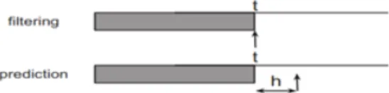
P(St+h|St+h−1). . . P(St+1|St).P(St|O1:t) (6) Firstly belief state should be calculated. For calculating the belief state the Forward Algorithm can be directly applied with the purpose of optimal filtering. Here filtering means reducing the noise by considering P(St|O1:t)overP(St|Ot)[15].
After finding the belief state calculating the prediction probability is just a matter of power up the transition matrix (A) and apply over the belief state. The two steps can be shown graphically as in Figure 5.
Figure 5: Graphical representation filtering and prediction [15]
4. EVALUATION
To assess the accuracy of the prediction of the system four types of measures [16] can be used (i.e. precision, recall, f-measure and false positive rate).
Precision: fraction of correctly predicted failures in comparison to all failure warnings.
Recall: fraction of correctly predicted failures in comparison to the total number of failures.
F-measure:harmonic mean of precision and recall.
False positive rate: fraction of false alarms with comparison to all non-failures.
Table 2: ACCURACY MEASUREMENTS
In order to calculate these measures, the matrix shown in Table 2 (a) is formed and the formulas in Table 2 (b) are used to calculate the above mentioned measures.
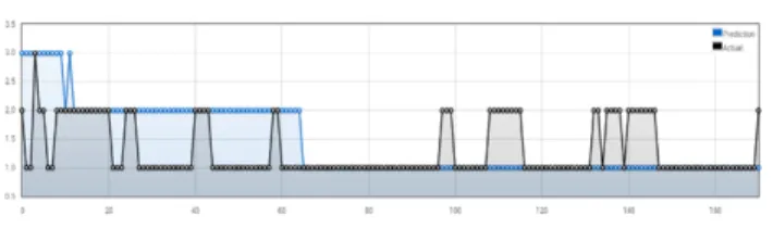
For the evaluation shown in Figure 6: the model has been trained with the data of ten weeks and prediction has been done for approximately ten hours.
The calculated precision is 0.09, recall is 1.0, false positive rate is 0.05 and F-measure is 0.166. Overall accuracy for this data set is about 64%. For the targeted prediction time box
Figure 6: Prediction results for ten hours the confusion matrix is shown in Table 3.
Table 3: CONFUSION MATRIX
Though here the precision is a low value as shown in Figure 6 too, the system identifies the severe levels closer to the due actual point. Other than that false positive rate is very low indicating a feature of an accurate failure prediction system.
5. DISCUSSION
Software failures are badly affecting the system reliability, which is a major quality factor in ISO/IEC 9126 quality model. This paper provides a solution for this problem by introducing a failure prediction mechanism to ensure fault-free execution of web services. In this research, a machine learning approach is used with HMM, which is trained with a vast collection of log file data of a web service. Predicting comprises two steps. First, it calculates the belief state by optimal filtering and then the prediction algorithm is applied. Further the implemented system is capable of predicting future states of the web service in three different severity levels (i.e. 1, 2 & 3) for the next ten hours.
This paper deals with the time component by making them equidistant (i.e. when applying HMM based prediction errors are assumed to be equidistant. As the log files contains silent zones it is challenging to deal with them for an accurate pre-diction. To meet a higher accuracy in this approach the system should be in one particular maintenance level throughout the whole period (i.e. from training period to prediction period). Otherwise the same trained HMM becomes inapplicable for all the predictions. Further, to have better results, determining the system state against the error observation should be made by a more reliable method rather collecting it from a human expert.
As future work, tuning the model for more accurate pre-dictions is intended to be done, and the system would be integrated with a module which provides the current system states automatically.
ACKNOWLEDGMENT
This research was supported by CITeS(Center for Information Technology Services) of University of Moratuwa by providing the required log file data and the other relevant information and
Faculty of Information Technology,University of Moratuwa by facilitating all the guidance.Further, the support given by Mr. Nadeesha Ranaweera, System Engineer, CITeS (Center for Information Technology Services) of University of Moratuwa and Mr. Channa Alwis, System Maintenance Engineer, Faculty of Information Technology, University of Moratuwa to carry out the research is also highly appreciated.
References
[1] Mark Endreiet al, Patterns: ServiceOriented Architecture and Web Ser-vices, IBM. April 2014.
[2] Sandeep Dalal and Dr. Rajender Singh Chhillar, Case Studies of Most Common and Severe Types of Software System Failure,International Jour-nal of Advanced Research inComputer Science and Software Engineering, Volume 2, Issue 8, August 2012.
[3] Lorin J. May, Major Causes of Software Project Failures,KjetilNrvag, An Introduction to Fault-Tolerant Systems, Norwegian University of Science and Technology, IDI Technical Report 6/99, Revised July 2000. [4] Jake Chapman,System failureWhy governments mustlearn to think
differ-ently, 2004.
[5] ”Issues for Nagios monitoring” [online], Available:https://www.drupal. org/project/issues/nagios.
[6] Yinglung Liang and RamendraSahoo, Failure Prediction in IBM Blue-Gene/LEvent Logs, Seventh IEEE International Conference on Data Min-ing, 2007.
[7] Felix Salfner and MiroslawMalek, Using Hidden Semi-Markov Models for Effective Online Failure Prediction, Institute of computer science, Humboldt University of Berlin, 2007.
[8] Yukihiro Watanabe and Yasuhide Matsumoto, Online Failure Prediction in Cloud Data Centers, Fujitsu Scientific & Technical Journal, January 2014. [9] MD.OsmanGani, Hasan Sarwar and Chowdhury Mofizur Rahman, Pre-diction of State of Wireless Network UsingMarkov and Hidden Markov Model, Journal of Networks, Vol. 4, No. 10, December 2009.
[10] Yin Wang, Software Failure Avoidance Using Discrete Control Theory, University of Michigan, 2009.
[11] L. R. Rabiner. A tutorial on hidden Markov models and selected applications in speech recognition. Proceedings ofthe IEEE, 77(2):257286, Feb. 1989.
[12] Felix Salfner, Maren Lenk, and MiroslawMalek, A Survey of Online Failure Prediction Methods, Humboldt University Berlin.
[13] Felix Salfner, Predicting Failures with Hidden Markov Models, Hum-boldt University Berlin.
[14] Kevin P. Murphy Machine Learning, A Probabilistic Perspective, The MIT Press Cambridge, Massachusetts London, England, 2012.
[15] Felix Salfner and Steffen Tschirpke, Error Log Processing for Accurate Failure Prediction[online], Available: https://www.usenix.org/legacy/event/ wasl08/tech/full papers/salfner/salfner html/index.html
![Figure 3: Errors, Faults & Failures [14]](https://thumb-us.123doks.com/thumbv2/123dok_us/536226.2563282/3.892.534.762.153.359/figure-errors-faults-amp-failures.webp)