Southern Methodist University
SMU Scholar
Statistical Science Theses and Dissertations Statistical Science
Spring 2018
Developing Statistical Methods For Data From
Platforms Measuring Gene Expression
Gaoxiang Jia
Southern Methodist University, [email protected]
Follow this and additional works at:https://scholar.smu.edu/hum_sci_statisticalscience_etds Part of theApplied Statistics Commons,Biostatistics Commons,Statistical Methodology Commons, and theStatistical Models Commons
This Dissertation is brought to you for free and open access by the Statistical Science at SMU Scholar. It has been accepted for inclusion in Statistical Science Theses and Dissertations by an authorized administrator of SMU Scholar. For more information, please visithttp://digitalrepository.smu.edu.
Recommended Citation
Jia, Gaoxiang, "Developing Statistical Methods For Data From Platforms Measuring Gene Expression" (2018).Statistical Science Theses and Dissertations. 1.
DEVELOPING STATISTICAL METHODS FOR DATA FROM PLATFORMS MEASURING GENE EXPRESSION
Approved by:
Dr. Xinlei Wang Professor of Statistics
Dr. Guanghua Xiao
Associate Professor of Biostatistics Dr. Daniel Heitjan
Professor of Biostatistics Dr. Lynne Stokes
DEVELOPING STATISTICAL METHODS FOR DATA FROM PLATFORMS MEASURING GENE EXPRESSION A Dissertation Presented to the Graduate Faculty of the
Dedman College of Humanities and Sciences Southern Methodist University
in
Partial Fulfillment of the Requirements for the degree of
Doctor of Philosophy with a
Major in Biostatistics by
Gaoxiang Jia
B.S., Shandong University, China, 2012
M.S., University of Texas Southwestern Medical Center, 2014 M.S., Southern Methodist University, 2017
Copyright (2018) Gaoxiang Jia All Rights Reserved
ACKNOWLEDGMENTS
Firstly, I would like to express my sincere gratitude to my advisors Drs. Xinlei Wang and Guanghua Xiao. They are the greatest mentors I could imagine: worked with me closely on my research and always provided the help and advice I needed. Their enthusiasm for statistics and science inspired me in all the time of my research. Without their training, I would not be able to become a statistician. They do not only train me in statistics, but also showed me how to treat people with respect and kindness.
Secondly, I would like to thank the rest of my thesis committee members Drs. Daniel Heitjan and Lynne Stokes, for their insightful comments on my dissertation and dedication to organizing this new joint biostatistics PhD program between SMU and UTSW. I also want to thank all the other faculty members in the Department of Statistical Science at SMU for their excellent teaching and help during my PhD study. My appreciation also goes to the faculty members who have helped me during my research and statistical consulting projects in the Department of Clinical Science at UTSW.
I would also like to thank my friends Dateng Li, Zhiyun Ge and Zhengyang Zhou for helping me on my coursework and research. Thanks for making my life at SMU enjoyable even when the pressure from courses and research projects is high.
I would like to thank my friends Kai Huang, Tao Wang and his wife, Yulei Zhang and his wife, Yandan Yang, Yixun Xing, Xue Li, Lin Qiu and Xiujun Zhu for their help on my application to the PhD programs at UTSW or SMU and/or their suggestions and encour-agement on my career.
Last but not the least, I would like to express my gratitude to my wife Jinyan Chan, my parents and other family members for always loving, supporting and believing in me.
Jia, Gaoxiang B.S., Shandong University, China, 2012
M.S., University of Texas Southwestern Medical Center, 2014 M.S., Southern Methodist University, 2017
Developing Statistical Methods for Data from Platforms Measuring Gene Expression
Doctor of Philosophy degree conferred May 19, 2018 Dissertation completed February 19, 2018
This research contains two topics: (1) PBNPA: a permutation-based non-parametric analysis of CRISPR screen data; (2) RCRnorm: an integrated system of random-coefficient hierarchical regression models for normalizing NanoString nCounter data from FFPE sam-ples.
Clustered regularly-interspaced short palindromic repeats (CRISPR) screens are usually implemented in cultured cells to identify genes with critical functions. Although several methods have been developed or adapted to analyze CRISPR screening data, no single spe-cific algorithm has gained popularity. Thus, rigorous procedures are needed to overcome the shortcomings of existing algorithms. We developed a Permutation-Based Non-Parametric Analysis (PBNPA) algorithm, which computes p-values at the gene level by permuting sgRNA labels, and thus it avoids restrictive distributional assumptions. Although PBNPA is designed to analyze CRISPR data, it can also be applied to analyze genetic screens im-plemented with siRNAs or shRNAs and drug screens. We compared the performance of PBNPA with competing methods on simulated data as well as on real data. PBNPA out-performed recent methods designed for CRISPR screen analysis, as well as methods used for analyzing other functional genomics screens, in terms of Receiver Operating Characteristics (ROC) curves and False Discovery Rate (FDR) control for simulated data under various
settings. Remarkably, the PBNPA algorithm showed better consistency and FDR control on published real data as well.
Formalin-fixed, paraffin-embedded (FFPE) samples have great potential for biomarker discovery, retrospective studies, and diagnosis/prognosis of diseases. However, their appli-cation is hindered by the unsatisfactory performance of traditional gene expression profiling techniques on damaged RNAs. NanoString nCounter platform is well suited for profiling of FFPE samples and measures gene expression with high sensitivity, which may greatly facil-itate realization of scientific and clinical values of FFPE samples. However, methodological development for normalization, a critical step when analyzing this type of data, is far be-hind that for traditional technologies such as microarray. Existing methods designed for the platform use information from different types of internal controls separately and rely on an overly-simplified assumption that expression of housekeeping genes is constant across samples for global scaling. We construct an integrated system of random-coefficient hierarchical re-gression models to capture main patterns and characteristics observed from NanoString data of FFPE samples, and develop a Bayesian approach to estimate parameters and normalize gene expression across samples. Our method, labeled RCRnorm, incorporates information from all aspects of the experimental design, and simultaneously removes biases from various sources. Further, it eliminates the unrealistic assumption on housekeeping genes and offers great interpretability. Simulation and applications showed its superior performance.
TABLE OF CONTENTS
CHAPTER
1. PBNPA: A PERMUTATION-BASED NON-PARAMETRIC ANALYSIS OF
1.1. Introduction . . . 1
1.1.1. CRISPR mediated genomic screens and other type of genomic screens 1 1.1.2. Review of existing methods for analyzing CRISPR screen data . . . 2
1.1.3. Motivation of our study . . . 4
1.1.4. Research overview. . . 4
1.2. Methods . . . 5
1.2.1. A permutation-based non-parametric method for calculating p -1.2.2. Combiningp-values to handle replicates . . . 6
1.3. Simulation studies . . . 6
1.3.1. Simulation strategy . . . 6
1.3.2. Positive selection performance . . . 9
1.3.3. Negative selection performance . . . 9
1.4. Comparison of recall, precision and estimation of pvalues . . . 14
1.4.1. Handling replicates . . . 15
1.5. Real data applications . . . 17
1.5.1. Consistency between replicates . . . 17
1.5.2. FDR control . . . 19
1.6. Discussion . . . 19
LISTOFFIGURES... x
LISTOFTABLES... xi
CRISPRSCREENDATA... 1
1.7. R package . . . 21
2. RCRNORM: AN INTEGRATED SYSTEM OF RANDOM-COEFFICIENT 2.1. Introduction . . . 23
2.2. Motivating example . . . 27
2.2.1. Data description . . . 27
2.2.2. Exploratory analysis . . . 29
2.2.3. Proposed data model based on RCR . . . 33
2.3. Bayesian approach . . . 36
2.3.1. Full probability model . . . 36
2.3.2. Prior specification . . . 37
2.3.3. Posterior computation and Bayesian inference. . . 38
2.4. Simulation . . . 38
2.4.1. Settings . . . 38
2.4.2. Results . . . 40
2.5. Real data applications . . . 43
2.5.1. Lung cancer data . . . 43
2.5.2. Colorectal cancer data . . . 49
2.6. Discussion . . . 50
2.7. R package . . . 53
APPENDIX A. PBNPA: A PERMUTATION-BASED NON-PARAMETRIC ANALYSIS OF A.1. Figures . . . 54
A.2. R package code for PBNPA. . . 54
HIERARCHICALREGRESSIONMODELSFORNORMALIZING NOSTRINGNCOUNTERDATAFROMFFPESAMPLES... 23
B.1. Tables and figures . . . 63
B.1.1. Additional information about lung cancer data . . . 63
B.1.2. Additional simulation results . . . 64
B.1.3. Results for colorectal cancer data . . . 64
B.2. Full conditionals . . . 64
B.3. R package code for RCRnorm . . . 72
B. RCRNORM:ANINTEGRATEDSYSTEMOFRANDOM-COEFFICIENT HIERARCHICALREGRESSIONMODELSFORNORMALIZING NANOS-TRINGNCOUNTERDATAFROMFFPESAMPLES... 63
LIST OF FIGURES
Figure Page
1.1 Simulation evaluation of positive selection performance. . . 10
1.2 Simulation evaluation of positive selection performance. . . 11
1.3 Simulation evaluation of negative selection performance. . . 12
1.4 Simulation evaluation of negative selection performance. . . 13
1.5 Simulation evaluation of positive selection performance. . . 16
1.6 Comparing consistency of MAGeCK and PBNPA on replicates. . . 18
2.1 Exploratory analysis of lung cancer data. . . 31
2.2 Simulation study I . . . 42
2.3 Simulation study II . . . 44
2.4 Simulation study III . . . 45
2.5 Lung cancer data: posterior densities of global parameters . . . 46
A.1 Simulation evaluation of positive selection performance. . . 55
A.2 Simulation evaluation of positive selection performance. . . 56
A.3 Simulation evaluation of negative selection performance. . . 57
A.4 Simulation evaluation of negative selection performance. . . 58
A.5 Simulation evaluation of negative selection performance based on recall, precision and F_1 . . . 59
B.1 Lung caner data: read counts of 6 positive controls . . . 64
B.2 Simulation study I . . . 65
B.3 Simulation study II . . . 66
B.4 Simulation study III . . . 67
LIST OF TABLES
Table Page
1.1 Comparison of FDR control between MAGeCK and PBNPA . . . 19
2.1 Lung cancer data: posterior summary statistics . . . 45
2.2 Lung cancer data: summary statistics of Pearson correlation coefficients . . . 48
2.3 Colorectal cancer data . . . 50
B.1 Lung cancer data: data structure from the NanoString nCounter platform . . . 63
Chapter 1
PBNPA: A PERMUTATION-BASED NON-PARAMETRIC ANALYSIS OF CRISPR SCREEN DATA
1.1. Introduction
1.1.1. CRISPR mediated genomic screens and other type of genomic screens
The CRISPR (clustered regularly-interspaced short palindromic repeats) interference technique is widely used in biomedical studies to investigate gene functions. Large-scale screening with this technique has become a powerful tool in identifying cancer-promoting genes, drug-resistant genes, and genes that play pivotal roles in various biological processes (Shalem et al.,2015;Hart et al.,2015;Wang et al.,2014). The CRISPR/Cas9 system is com-posed of sgRNAs (single guide RNA) and Cas9s (CRISPR associated protein 9); an sgRNA contains around a 20-bp guide sequence that complements a DNA sequence and thus targets a gene of interest, and a Cas9 is a nuclease that induces double-strand breaks in the DNA and results in non-homologous end joining (NHEJ) repair. NHEJ is an error-prone repair mechanism that usually introduces an indel mutation that is highly likely to cause a coding frameshift, which leads to a premature stop codon and initiates the nonsense-mediated de-cay of the transcribed mRNA (Shalem et al., 2015). Thus, the CRISPR system abolishes the gene function by interfering with gene expression from the DNA level. This is more powerful than siRNA (small interfering RNA) or shRNA (short hairpin RNA) screens. An siRNA contains 20 ~ 25 bp short synthesized RNAs that function in the RNA interference pathway, and it cannot be integrated into a host genome. An shRNA contains synthesized double-stranded RNA molecules with a tight hairpin turn, which can be integrated into
2014). All three types of screens are usually implemented on cultured cells: siRNA screens are carried out in multi-well plates with each well containing one or several siRNAs tar-geting the same gene, and the signal in each well is collected as the read for that well; by contrast, CRISPR and shRNA screens are carried out in a pooled manner, where a mix-ture of lentivirus that contains RNAi reagents (either shRNA or sgRNA) targeting different genes is transfected into the same plate of cultured cells, and the microarray or next gen-eration sequencing (NGS) technique can be used to collect reads. Cas9-sgRNA screens are performed with pre-designed sgRNA libraries that contain sgRNA redundancy. Generally, multiple sgRNAs (usually ranging from 3-10) with different sequences that target distinct locations on the same gene are utilized to ensure screening accuracy (Shalem et al., 2015). All genome-wide CRISPR screens use cell growth as a phenotypic measure. Based on the goal of the screens, they can be divided into positive selection screens and negative selection screens (Shalem et al.,2014). Positive screens aim to identify genes that inhibit cell growth in certain circumstances or that sensitize cells to a drug treatment or toxin. For example, genes protecting cells against toxins, which are likely to be receptors for the toxins, or genes involved in downstream signaling pathways (Koike-Yusa et al., 2014), may be targeted by positive screens. Under a strong selective pressure, cells with sgRNAs that confer resistance against that pressure would be enriched, and thus their signals are often strong and easy to detect. Negative selection screens aim to identify genes that promote cell growth or house-keeping genes (Morgens et al., 2016). In this scenario, cells that carry sgRNAs targeting such genes will be depleted during selection. Signals from negative screens are typically not as strong as those from positive screens, because the depletion level is usually mild and the number of depleted sgRNAs is large when considering the number of housekeeping genes (and thus they can be hard to separate from the background.)
1.1.2. Review of existing methods for analyzing CRISPR screen data
There are existing methods that can be used to analyze genome-wide RNA interfering screening results, including RSA (Konig et al.,2007), RIGER (Luo et al.,2008), MAGeCK
(Li et al.,2014), ScreenBEAM (Yu et al.,2016), etc. The Redundant siRNA Activity (RSA) method was originally developed to analyze data generated by large-scale small interfering RNA (siRNA) screens in mammalian cells (Konig et al., 2007). RSA calculates a p-value
for each gene based on an iterative hypergeometric distribution formula, where a smaller p-value indicates the gene is more likely to have higher activity. RNAi Gene Enrichment Ranking (RIGER) was originally designed to identify essential cell genes in genome-scale pooled shRNA screens (Luo et al., 2008). It calculates the rank of each sgRNA based on a signal-to-noise metric and then synthesizes information on sgRNAs targeting the same gene in a way similar to that of Gene Set Enrichment Analysis to rank genes (Subramanian
et al., 2005). Model-based Analysis of Genome-wide CRISPR/Cas9 Knockout (MAGeCK)
and Screening Bayesian Evaluation and Analysis Method (ScreenBEAM) were both designed to analyze CRISPR screen data. MAGeCK evaluates sgRNAs based on p-values calculated from fitting a negative binomial model (Li et al., 2014), and then the ranks of sgRNAs tar-geting the same gene are combined with a modified version of robust ranking aggregation (RRA) called -RRA. ScreenBEAM assesses the gene level activity with Bayesian hierarchical models (Yu et al., 2016), in which within-gene variances were modeled as random effects. Among the above methods, RIGER, MAGeCK and ScreenBEAM can perform both positive and negative selection. In addition, several algorithms used for analysis of Next Generation Sequencing (NGS) data, such as edgeR (Robinson and McCarthy, 2010), DESeq (Anders and Huber, 2012) baySeq (Hardcastle and Kelly,2010), NOISeq (Tarazona et al.,2012) and SAMseq (Li and Tibshirani, 2013), can also be used to analyze RNAi screening data. Al-though such methods can only assign ranks at the sgRNA level, they can be used to conduct gene-level inference (Li et al., 2014) when combined with existing methods of integrating group information. It is worth noting that NOISeq and SAMseq both take nonparametric approaches. Unlike our method that is based on permutation, SAMseq mainly relies on the two-sample Wilcoxon statistic to estimate the significance; and NOISeq assesses the signif-icance of the treatment effect with the reference distribution generated by comparing reads of each gene in samples under the same condition.
1.1.3. Motivation of our study
Although many CRISPR screen analysis methods are available, no single specific algo-rithm has gained popularity from researchers, mainly due to one or more of the drawbacks listed below: (1) Distributions assumed are doubtful or incorrect and thus incapable of mod-eling data variability from different sources. Researchers generally use negative binomial or Poisson distributions to model read counts from NGS (Seyednasrollah et al.,2015). However, these distributions do not reflect certain characteristics of NGS data generating processes and are weak in handling over-dispersion. (2) Most studies compared their model performance using some ‘oracle’ datasets. However, the performance may be compromised when general-izing these methods to datasets from different conditions or platforms. This is reflected by the fact that the number of consistently identified genes across different algorithms is often small (Diaz et al.,2015). (3) Published methods usually have loose or no false discovery rate (FDR) control. FDR reflects the rate of type I errors when performing multiple hypothesis tests and influences the credibility of the tests if not carefully controlled. False discovery is a big concern for functional genomic studies when a large number of statistical tests are performed (Pawitan et al., 2005). The above-mentioned methods tend to overlook FDR or be ineffective in controlling it, as will be shown in detail in the Real Data Application section. Without stringent FDR controlledp-values, it is difficult to evaluate the statistical
significance of selected genes. 1.1.4. Research overview
Our proposed method, Permutation-Based Non-Parametric Analysis (PBNPA) of CRISPR screen data, mitigates the three major drawbacks of existing CRISPR methods. First, PB-NPA computes p-values at the gene level by permuting sgRNA labels, and thus it avoids
restrictive distributional assumptions. Second, PBNPA shows superior performance to other algorithms in simulation using data generated to mimic the NGS sequencing process, which avoids overfitting based on specific datasets. Application to real data confirms better
con-sistency of PBNPA. Last, our data application reveals that PBNPA outperformed its com-petitors in terms of FDR control.
1.2. Methods
1.2.1. A permutation-based non-parametric method for calculating p-values for genes
In a CRISPR screen dataset, assume Yij is the read count for the jth sgRNA in the library under condition i, where j = 1,2,· · ·, J indexes sgRNAs in the library; and i = 0,1 indexes two experimental conditions, with i = 0 for the control and i = 1 for the treatment. We use Ig to denote the index set of the sgRNAs that target the same gene g and SGg=1Ig = {1,2,· · ·, J}, where g = 1,2,· · ·, G and G is the total number of genes in
the library. Raw read counts in each condition i were normalized by multiplying a factor of mean(PJj=0Y0j,PJj=1Y1j)/PJj=1Yij. This makes total read counts in each condition equal without losing any useful information. Our PBNPA algorithm is outlined below.
1. For each sgRNA j (j = 1,2,· · ·, J), calculate the natural logarithm fold change of normalized read counts: rj = log(Y1j/Y0j). Then for each gene g, use the median of
rj’s (j 2Ig) as theR score, denoted byRg.
2. Randomly permute gene labels while holding (Yoj, Y1j)pairs unchanged to get permu-tated R scores for each gene, denoted by R⇤
g1’s, where g = 1,2,· · ·, G.
3. Repeat step 2 for T times and pool all R⇤
gt’s over the T permutations and all genes to form a null distribution ofR.
4. Calculate the p value for gene g if it is a positively selected gene as:
p= (#of permuted R scores>Rg)/(total # of permuted R scores); and the value for gene if it is a negatively selected gene as:
5. After gettingpvalues for all genes, remove genes withpvalues smaller than a threshold,
which are considered to be significant genes. Then repeat step 2 and 3 to get the null distribution with significant genes removed. Get updated p values for each gene as
described in step 4.
6. Use the Benjamini-Hochberg procedure to control FDR (Benjamini and Hochberg, 1995).
In this algorithm, the median log fold change of sgRNAs targeting a gene is used as the score of that gene, which makes it more robust against any outliers and influences from potential off-target effects. In step 5, we remove a small portion of genes with the purpose of removing any significant genes to get a more accurate estimate of the null distribution , as the null distribution is likely to be distorted if these significant genes are kept in the permutation process.
1.2.2. Combining p-values to handle replicates
A CRISPR screen experiment may contain several replicates. We analyzed each replicate using the proposed algorithm and then employed Fisher’s method to combine p-values from
replicates for each gene (Brown, 1975; Rau et al., 2014). According to Fisher’s method, the statistic 2PSs=1lnpgs, withpgs representing gene g’spvalue from thesth replicate, follows an 2 distribution with 2S degrees of freedom under the null hypothesis H
o: gene g has no effect, from which a combined p value for each geneg is obtained (Brown, 1975).
1.3. Simulation studies 1.3.1. Simulation strategy
To mimic the nature of RNA-seq experiments, the read counts of all sgRNAs under a given condition were generated from a Dirichlet-multinomial (DM) distribution. Considering the experimental setup of CRISPR screening with RNA-seq, each sgRNA in a library can
(sequencing depth) is fixed. However, the literature indicates that multinomial distributions are inadequate to model the extra variability that is usually observed in NGS data (Chen and Li,2013; Bonafede et al., 2016). To account for over-dispersion, the probability vector of an NGS read falling into the different sgRNA categories is modeled as random variables from a Dirichlet distribution. After combining the multinomial model with the Dirichlet model, the mixture model is a Dirichlet-multinomial model with the probability mass function (PMF) shown below: f(Yi) = (Yi++ 1) ( i+) (Yi++ i+) J Y j=1 (Yij + ij) (Yij + 1) ( ij)
where Yi = [Yi1, Yi2,· · ·, YiJ], Yi+ =PJj Yij, i+ =PJj ij with ij’s being the parameters of the DM distribution; and E(Yij) = Yi+ iij+ and V ar(Yij) = Yi+ iij+(1 iij+)(Yi1+++i+i+) (Chen
and Li,2013;Tu,2014). Compared to the variance of the multinomial model, the variance of the DM model is increased by a factor of Yi++ i+
1+ i+ . When the total read countYi+ is fixed, i+
controls the degree of overdispersion with a smaller value indicating larger overdispersion. To simulate read counts for a screen experiment, we first generated 0j’s for a control sample from a negative binomial distribution N B(q, p) where q is the number of successful
trials to be reached andpis the probability of success in each trial. We setq = 3andp= 0.08 so that the generated DM read counts are right skewed, which approximately mimics real data. We link ij to the effect of sgRNA j through the relationship ij = exp(↵j + j ⇥i), where↵j loosely reflects the log mean read count under the control and j represents thejth sgRNA effect (i.e., the log difference in mean read count between the treatment and control). The total number of genes G was set to be 10000. For genes that have effects during the screen processes under different conditions (which are referred to as true hits), we first generated the sgRNA effects targeting gene g from a normal distribution, j ⇠ N(µg, 2) for j 2 Ig, g = 1,2, . . . , G, with gene-specific mean µg and constant standard deviation = 0.4 (0.4 was chosen to be close to the standard deviation estimated from real data); and then we forced all j’s for gene g to have the same sign as µg. The vector, which
contains different levels ofµg in our simulation, was set to be [1.5,1,0.5, 1, 2, 3], where a positive number indicates that a gene’s ablation promotes cell growth while a negative number indicates a gene is necessary for cell growth. The three levels of µg for each sign represent the high/medium/low effects of positively/negatively selected genes, respectively. There are 50 genes simulated from each level of µg. Thus, among the 10000 genes, there are 150 positively selected genes and 150 negatively selected genes. For those genes with no effects, j’s were set to be 0.
Off-target effects of CRISPR are often caused by unintended DNA cleavage at non-targeting sites as a result of mismatch between DNA and sgRNA (Cho et al., 2014). If an sgRNA is an off-target effect, its read count may either decrease, increase, or remain the same since most DNA sequences in the human genome have no known function. In our simulation, off-target j’s were simulated from N(0, 2) and then used to replace a certain proportion of randomly-selected on-target sgRNAs. The off-target rate of a library can be considered an important characteristic reflecting the quality of the library, which is determined by the algorithm used to design the sgRNAs (Xu et al., 2015). Although several experimental approaches exist, it is still challenging to get accurate estimates of sgRNA off-target rates (Wu et al.,2014; Zhang et al., 2015). Reported off-target rates vary greatly in the literature (Fu et al.,2013;Haeussler et al., 2016) and can range between 1% and 20% in most sgRNA libraries. Thus, we tested 4 off-target proportion values: 1%, 5%, 10% and 20%, to represent sgRNA libraries of different quality.
Besides the library quality, the number of sgRNAs per gene is another factor that is known to influence the screen performance dramatically. Thus, we varied the number of sgRNAs per gene from 2 to 6 as well.
With j’s simulated for all sgRNAs, we obtained 1j = 0jexp( j). Then we simulated
Yij from the DM distribution with ij’s from statistical packages ’multinomRob’ (Mebane Jr and Sekhon, 2009) and ’dirmult’ (Tvedebrink, 2010).
1.3.2. Positive selection performance
We compared the performance of PBNPA, RSA, ScreenBEAM and MAGeCK for the four different off-target rates (1%, 5%, 10%, 20%), as mentioned in the simulation strategy section, when there are 3 sgRNAs targeting each gene. A receiver operating characteristic (ROC) curve plots the true positive rate against the false positive rate of a binary classi-fier for different possible cut-off points and visualizes the performance of the classifier. As shown in Figure 1.1, PBNPA works better for positive screening than RSA, MAGeCK and ScreenBEAM in terms of the ROC curve and area under the curve (AUC), regardless of the off-target proportion. Also, all the algorithms show worse performance with an increasing off-target rate except for RSA, whose AUC increases from 0.592 to 0.637. Figure 1.2 indi-cates that PBNPA outperforms the other algorithms with varying numbers of sgRNAs per gene from 2 to 5. As expected, the AUC of each method increases with an increasing number of sgRNAs per gene, as more sgRNAs enable better estimation of gene effects.
As we have discussed previously, i+ controls the degree of over-dispersion. To check the
performance of the algorithms with an increased over-dispersion level, we divided every ij by 10 and report the results in FiguresA.1 andA.2 of Appendix: the performance of nearly all algorithms decreases compared with the low over-dispersion setting, but the performance of PBNPA and ScreenBEAM is comparable, and it is better than RSA and MAGeCK.
1.3.3. Negative selection performance
For negative selection, PBNPA and RSA have similar AUCs and perform better than MAGeCK and ScreenBEAM when the proportion of off-target sgRNAs is low, as shown in Figure1.3. When the proportion of off-target sgRNAs increases, RSA shows some advantage over PBNPA and is robust against this increase. Figure 1.4 shows that when we fix the off -target proportion at 10% and vary the number of sgRNAs per gene, PBNPA and RSA have comparable performance, and they are significantly better than MAGeCK and ScreenBEAM when the number of sgRNAs per gene is low.
Figure 1.1. Simulation evaluation of positive selection performance. ROC curves and AUCs are shown for different algorithms with an increasing offtarget proportion while the number of sgRNAs per gene is fixed at 3. Each curve represents the average of ROC curves for 50 simulated datasets and above.
Figure 1.2. Simulation evaluation of positive selection performance. ROC curves and AUCs are shown for different algorithms with an increasing number of sgRNAs per gene, while the off target proportion is fixed at 10%.
Figure 1.3. Simulation evaluation of negative selection performance. ROC curves and AUCs are shown for different algorithms with an increasing offtarget proportion, while the number of sgRNAs per gene is fixed at 3.
Figure 1.4. Simulation evaluation of negative selection performance. ROC curves and AUCs are shown for different algorithms with an increasing number of sgRNAs per gene, while the off target proportion is fixed at 10%.
In the setting of high over-dispersion, RSA is the best among all and PBNPA is only second to RSA with increasing off-target proportion in the simulated datasets, as shown in Figure A.3 (Appendix). Figure A.4 (Appendix) shows that when we fix the off-target proportion and vary the number of sgRNAs per gene, RSA is slightly better than PBNPA, and they are better than the other two algorithms across different numbers of sgRNAs per gene. Overall, for negative selection, RSA seems to be the winner; but PBNPA provides quite close or comparable performance to RSA, which is much better than MAGeCK and ScreenBEAM.
1.4. Comparison of recall, precision and estimation of p values
When multiple statistical tests are performed simultaneously in the analysis of a dataset, adjustment ofpvalues is needed. Among the four algorithms, RSA does not provide a method
to adjust for multiple comparison. We applied the Benjamini-Hochberg (BH) procedure
(Benjamini and Hochberg, 1995) to the results from RSA and obtained FDR-adjusted p
values. The other three methods use the BH procedure by default. Then we controlled FDR at 5% and compared recall (percent of identified true hits among all true hits), precision (percent of identified true hits among all selected genes) andF1 of the four algorithms, where
F1 is a metric that balances recall and precision and is defined as F1 = 2⇥ recallrecall⇥+precisionprecision.
To our surprise, when FDR was controlled at 5%, neither RSA nor ScreenBEAM was able to identify any significant genes. Actually, under most settings, all genes in the RSA results had an adjusted p-value of 1. This suggests that RSA and ScreenBEAM cannot accurately
estimate the statistical significance of the genes. Thus, we compared the recall, precision and F1 of PBNPA and MAGeCK. Figure 1.5 shows the recall, precision and F1 of PBNPA
and MAGeCK for different combinations of sgRNA number per gene (2, 3, 4, 5, 6) and off-target rates (1%, 5%, 10%, 20%) for positive screens. From the bottom panel of Figure 1.5, it is clear that under most settings, F1 of PBNPA is the same as or slightly better
than that of MAGeCK. However, the recall of PBNPA is significantly better than that of MAGeCK, especially when the number of sgRNAs per gene is small. In the middle
panel, MAGeCK consistently maintains very high precision across all the settings. However, MAGeCK tends to be too conservative in identifying true hits and may show a lack of power. Note that when the off-target rate is high (20%) with 2 sgRNAs per gene, MAGeCK has a recall rate of less than 10%, where it cannot identify any true hits at all in some simulated datasets. In screening experiments, after the genome-wide screening, a secondary screening will typically be used to validate hits from the first round (Miles et al.,2016). This highlights the importance of the recall rate: those false positives are likely to be removed in the secondary screening, while those false negatives can be crucial genes that will be missed permanently. Nearly the same pattern can be observed for negative screens, as shown in Figure A.5 (Appendix). Thus, PBNPA provides the most accurate estimation of adjustedp
values among the four algorithms and also offers optimal recall rates. 1.4.1. Handling replicates
The comparisons we have discussed above are based on simulated data with no replicates. For low-quality screens, replicates are typically used to increase the power of identification. To handle screens with replicates, we propose to use Fisher’s method to combine p values,
as mentioned in the Methods section, followed by FDR adjustment. We simulated replicate datasets with parameters of the DM distribution set as ij
5 , which has higher over-dispersion
than the DM distribution with ij and so may represent data of low quality. We evaluated 3 simulated replicates independently. Among the 150 positively selected genes, the analysis of individual replicates gives the following results (i.e., number of true hits identified/number of genes identified by PBNPA) with FDR controlled at 5%: 6/7, 9/11, and 8/9, respectively. After combining p values for the first two replicates, the result is 72/86. After combining p values for all three replicates, the result is 96/111. It is evident that PBNPA shows
Figure 1.5. Simulation evaluation of positive selection performance based on recall, precision andF1 for different combinations of sgRNA number per gene (2~6) and offtarget ratio. Each
bar represents the average of 50 simulated datasets and the standard error is indicated on the bar.
1.5. Real data applications 1.5.1. Consistency between replicates
Although the performance of various algorithms usually does not differ greatly in simula-tion studies, they tend to give quite different inferences on real data. This can be due to the fact that a simulation is not an exact reproduction of the complex data generation process in the real world. This phenomenon is also observed in algorithms analyzing CRISPR data
(Diaz et al., 2015). From the simulation study, we have found that PBNPA and MAGeCK
are handy to use and give better overall performance than the other two algorithms. Thus, we used datasets from two recently published articles to evaluate the consistency between these two algorithms as well as the consistency of the same algorithm on different replicates from the same experiment, since a good algorithm should give highly similar results on repli-cates of the same experiment. The KBM7 dataset is from a study with two replirepli-cates and 10 sgRNAs per gene, which aims to identify essential genes in the human genome to reveal genes that are oncogenic drivers or lineage specifiers (Wang et al., 2015). As shown in the upper panel of Figure 1.6, the identified hits are highly overlapped between the two algorithms for the same replicate, as well as between the two replicates with the same algorithm. This indicates both algorithms perform well on this dataset with high consistency. The Toxo-plasma dataset is from a study with four replicates, which aims to identify essential genes of parasites for infection of human fibroblasts (Sidik et al.,2016). The library was designed to target more than 8000 protein coding genes inT. gondii with 10 sgRNAs per gene. For this dataset, the number of consistently identified genes for PBNPA is significantly higher than that identified by MAGeCK among the 4 replicates, as is shown in the middle and bottom panels of Figure1.6. For PBNPA, there are 19 genes consistently identified in all four repli-cates and 80 genes consistently identified in at least three replirepli-cates. However, for MAGeCK there is no gene identified in all four replicates and only 11 genes consistently identified in at least three replicates. This is strong evidence that PBNPA has superior consistency and better FDR control than MAGeCK.
Figure 1.6. Comparing consistency of MAGeCK and PBNPA on replicates using real data. Upper panel: overlap of PBNPA and MAGeCK results on replicates 1 and 2 of the KBM7 dataset. Middle panel: overlap of PBNPA results on the four replicates of Toxoplasma. Bottom panel: overlap of MAGeCK results on the four replicates of Toxoplasma.
1.5.2. FDR control
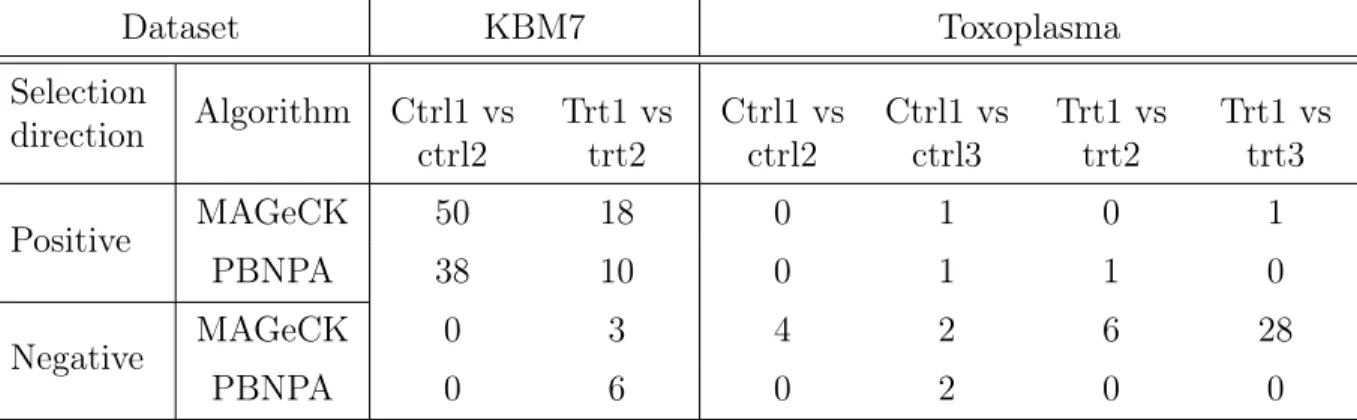
Control of FDR is also studied by comparing control vs control or treatment vs treatment read counts between replicates, as no genes should be identified in this comparison. For the KBM7 dataset, we analyzed controls vs controls or treatment vs treatment with the two algorithms and found that PBNPA has fewer falsely identified genes compared with MAGeCK, as shown in Table 1.1. For the Toxoplasma dataset, the results also indicated PBNPA had fewer falsely identified genes than MAGeCK which is showed in Table 1.1.
Dataset KBM7 Toxoplasma Selection direction Algorithm Ctrl1 vsctrl2 Trt1 vstrt2 Ctrl1 vsctrl2 Ctrl1 vsctrl3 Trt1 vstrt2 Trt1 vstrt3 Positive MAGeCK 50 18 0 1 0 1 PBNPA 38 10 0 1 1 0 Negative MAGeCK 0 3 4 2 6 28 PBNPA 0 6 0 2 0 0
Table 1.1. Comparison of FDR control between MAGeCK and PBNPA
1.6. Discussion
The similarities and differences in performance of the two algorithms, MAGeCK and PBNPA, on the two real datasets can be explained below. In the KBM7 dataset, each gene is targeted by 10 sgRNAs. From our simulation study, 10 sgRNAs per gene should be sufficient to give reliable inference on the hits. Thus, these two algorithms give highly similar results. For the Toxoplasma dataset, although there are 10 sgRNAs designed for each gene, the algorithm used to design sgRNAs is optimized for human genes not for Toxoplasma, which, we conjecture, would deteriorate the efficiency of sgRNAs in the screen. In addition, the screening pipeline for Toxoplasma differs from that for cultured human cells, which may induce unknown variability in the data. Based on the above rationale, we conclude that
methods (RSA and ScreenBEAM) did not perform well on these real data, which agrees with our findings from simulation. In particular, RSA showed poor performance in controlling FDR; for example, in the KBM7 dataset, when we compared ctrl1 vs. ctrl2, RSA claimed more than 90% of the genes are significant when controlling FDR at 5% for positive selection. This is also consistent with an observation in the MAGeCK paper (Li et al.,2014) that RSA has a high FDR.
While researchers typically use gene-specific null distributions in their permutation pro-cedures, we employed a common null probability distribution for all genes in PBNPA. We find that this gives similar or even slightly better performance than using gene-specific null distributions. However, building a common null distribution for all genes substantially saves computation time over building gene specific null distributions. For example: if there are 10,000 genes and we permute 10 times, we can get a common null distribution for all genes based on 10000⇥ 10=100,000 replicates; but we need to permute 100,000 times if we want an individual null distribution for each gene based on the same number of replicates. Here, using a common null distribution saves 10,000 times as much computation time as using gene-specific null distributions.
Although our algorithm is designed to analyze CRISPR data, it can also be applied to analyze genetic screens implemented with siRNAs or shRNAs and drug screens, which all generate data with structures similar to those in CRISPR screens. The idea of doing permutation twice, with significant genes from the first round removed to get a more accurate null distribution, could be used by other studies where p values are mainly generated from a permutation process. We note that there are supervised methods of analyzing CRISPR data, which need previous knowledge to estimate the background noise in the platform and variability in the data (Hart and Moffat, 2016). Such methods are suitable in situations when reliable previous screening results are available.
To the best of our knowledge, our paper is the first study to compare the performance of several algorithms with simulated datasets. With the known ground truth, we showed the overall superiority of our PBNPA algorithm compared to several existing methods in
analyzing CRISPR data, which is also verified by the real data studies. The behaviors of each algorithm are revealed from simulation studies, which could help researchers select the most appropriate algorithm to analyze CRISPR data.
Although there are many existing algorithms available for analyzing CRISPR data, re-searchers are particularly interested in new algorithms that can give consistent and reliable results with a small number of sgRNAs per gene and a low sequencing depth and that are not sensitive to platforms, which will facilitate genome-scale screens while lowering the cost. Our PBNPA algorithm is a step toward achieving this goal.
1.7. R package
We created an R package to implement PBNPA. This package is available at at CRAN: https://cran.r-project.org/web/packages/PBNPA/index.html.
The main function in the package named ’PBNPA’. This function uses the raw read count data for CRISPR (Clustered Regularly Interspaced Short Palindromic Repeats) screens and conducts statistical analysis for permutation based non-parametric analysis of CRISPR screen data. This function can also be used to analyze data from other types of functional genomics screens such as siRNA screen or shRNA screen. Drug screens or microarray ex-pression data, if they have structures similar to what this algorithm is designed for, can also be analyzed with this function as the algorithm has no specific distributional assumptions for the data and p-values are calculated from a permutation based procedure. It can
han-dle data with multiple replicates. After executing the function, a list of 5 elements will be returned. The first element is pos.gene, which is the index of genes identified as hits for
positive screen by controlling FDR at the selected level; the second element is pos.number,
which is the number of genes identified as hits for positive screening; The third element is
neg.gene, which is the index of genes identified as hits for negative screen by controlling
FDR at the selected level; the fourth element is neg.number, which is the number of genes
un-adjusted p-values and FDR adjusted p-values for all the genes (for both negative selection
Chapter 2
RCRNORM: AN INTEGRATED SYSTEM OF RANDOM-COEFFICIENT HIERARCHICAL REGRESSION MODELS FOR NORMALIZING NANOSTRING
NCOUNTER DATA FROM FFPE SAMPLES
2.1. Introduction
Formalin-fixed paraffin-embedded (FFPE) tissue samples are usually collected for diag-nostic purposes in clinical routines (Lüder Ripoli et al., 2016). Unlike freshly frozen (FF) tissue samples that must be frozen instantly after collection and then stored in freezers, FFPE samples can be stored at room temperature and kept for a long time. Due to the ease of handling and inexpensive storage (Perlmutter et al., 2004), numerous FFPE tissue samples have been deposited into tissue banks and pathology laboratories around the world, and are readily available (Lüder Ripoli et al., 2016; Reis et al., 2011). Such samples are often accompanied by well documented patient information, disease status and long-term clinical follow up information. Further, there exist vast archives of specimens from which only FFPE, but no FF, samples can be obtained (e.g., specimens of a deceased patient). Thus, the ubiquity of FFPE samples has made them a highly valuable resource in biomedi-cal studies. In particular, FFPE samples have great potential for biomarker discovery, which can be critical for disease diagnosis, prognosis and treatment plan selection (Ludwig and Weinstein, 2005; Rosenfeld et al.,2008; Xie et al., 2011).
Despite advantages of FFPE samples, the formalin fixation process breaks RNA into small pieces with an average size of ⇠200nt and irreversible methylene crosslinks between RNAs and proteins may form that affect enzyme based downstream reactions (Masuda et al.,1999). The low quality of RNA from FFPE samples hinders reproducibility and sensitivity of assays
polymerase chain reaction (qPCR) which involves enzyme-mediated reverse transcription from mRNA to cDNA (Von Ahlfen et al.,2007). Thus, in order to exploit the vast collection of FFPE samples, robust assays are needed to enable and improve expression profiling in these samples.
In recent years, several methods/platforms have been developed for gene expression pro-filing in FFPE samples either at the genome-wide scale or for a subset of genes. April et al. developed a whole genome cDNA-mediated annealing, extension, selection, and ligation (WG-DASL) assay to perform gene expression profiling in FFPE samples (April et al.,2009). Iddawela et al. reported that WG-DASL assays could reliably probe gene expression levels in breast cancer FFPE samples (Iddawela et al.,2016). Abdueva et al. showed that Affymetrix microarrays could be used to probe gene expression signatures and perform differential ex-pression analysis with FFPE samples and obtained results comparable to those from unfixed tissues (Abdueva et al., 2010). Thompson et al. developed the HTG EdgeSeq chemistry platform that uses RNA extraction-free nuclease protection assay (qNPA), followed by the quantification of RNA molecules by next generation sequencing techniques such as RNA-seq, to profile microRNA and RNA in FFPE samples (Thompson et al.,2014).
Unlike whole genome expression profiling above, Paluch et al. developed targeted RNAseq that can selectively examine the abundance of immune related genes on archival FFPE sam-ples (Paluch et al., 2017). Usually, platforms for measuring expression levels of a subset of genes only are called medium-throughput platforms. Compared to the high-throughput (genome-wide) platforms, they often have better technical reproducibility and are more read-ily to use in clinical settings. For medium-throughput platforms, besides the probes for detecting genes of interest, there are usually probes designed for internal control, for exam-ple, negative controls, positive controls and housekeeping genes. Negative controls target no known sequence and should have zero count ideally; positive controls added to the reac-tion system have known amounts of RNA targets; and housekeeping genes maintain basic cell functions, with expression levels that minimally fluctuate across different individuals compared with other genes (Waggott et al.,2012). These internal controls can provide
infor-mation for adjusting for unwanted biological and technical effects that can mask the signal of interest.
Among the medium-throughput platforms, the NanoString nCounter is the most popular (Geiss et al., 2008). It is highly multiplexed – it can effectively detect up to 800 genes in a single tube in one run, which bridges the gap between genome-wide expression profiling by microarray or RNAseq and targeted profiling by qPCR (Kulkarni,2011). More importantly, the nCounter platform is a Clinical Laboratory Improvement Amendments (CLIA) certifiable assay (for Medicare & Medicaid Services et al.,2005), which could be translated into clinical settings.
Due to its importance in medium-throughput profiling, several analysis methods includ-ing NanoStrinclud-ingNorm, NAPPA and NanoStrinclud-ingDiff have been developed for the NanoString nCounter platform to normalize and extract gene expression levels from different samples. These algorithms are mainly focused on removing noise from each of the following three sources with the use of one specific type of internal controls: (1) lane-by-lane noise, which results from variation in experimental conditions (such as humidity, temperature, etc.) be-tween reaction systems, is estimated and removed using information from positive controls; (2) background noise, introduced by non-specific binding of the probes, is estimated and re-moved using negative controls; and (3) variation in sample loading amounts or difference in RNA degradation levels is evaluated using housekeeping genes (Waggott et al., 2012; Wang et al., 2016; Harbron and Wappett, 2015).
To be specific, NanoStringNorm is an R package that implements a normalization protocol recommended by the manufacturer’s guideline (Waggott et al.,2012). First, the lane-by-lane variation is removed by scaling the samples with a factor that makes summary statistics of positive control counts (e.g., mean, median, or geometric mean) equal across samples. Then background correction is performed by subtracting the read count with a statistic represent-ing the background noise, for example, the mean or maximum count of negative controls. Finally, the loading variation is adjusted by a factor calculated from housekeeping genes in the same way as in the first step. It is obvious that NanoStringNorm performs normalization
in an ad hoc way without any rigorous statistical model involved. NAPPA is perhaps the most commonly used algorithm by researchers to normalize NanoString data (Harbron and Wappett,2015), to the best of our knowledge. This algorithm adjusts the background noise with a truncated Poisson distribution and corrects the loading variation by fitting a sig-moidal curve while normalizing the lane-by-lane variation similarly as in NanoStringNorm. NanoStringDiff is originally designed for identifying differentially expressed genes based on the NanoString nCounter platform, but can be easily adapted for the purpose of normaliza-tion (Wang et al., 2016). NanoStringDiff fits a generalized linear model to the data, from which three factors are extracted from positive controls, negative controls and housekeeping genes to adjust for lane-by-lane variation, background noise and variation in the amount of input sample, respectively.
Although the three methods are designed for or can be used to normalize NanoString nCounter data, no meticulous research has been conducted to study the characteristics of this type of data from FFPE samples; and no simulation studies were carried out to evaluate their performance in normalizing such FFPE data. In addition, information provided by different types of internal controls is intermingled. For example, although positive controls are designed to measure the noise from varying experimental conditions, read counts from negative controls can also provide useful information about this type of noise. The current normalization methods ignore this fact and cannot make the best use of data. In addition, all current algorithms use housekeeping genes by assuming that their expression levels are constant between different samples or individuals. But this may be fallacious – biologists generally define housekeeping genes as those that do not vary much between different tissues of an individual, but they have not evaluated the stability of their expression levels from different individuals (Eisenberg and Levanon, 2013). Thus, advanced statistical modeling based on an integrated understanding of the nCounter system without restrictive model assumptions is needed to boost its application in clinical and academic research.
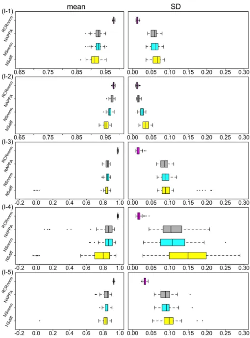
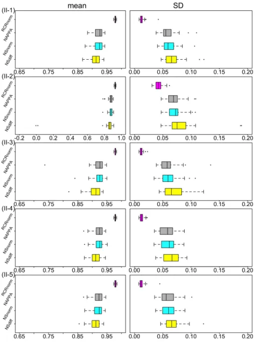
We begin by exploring key features of the NanoString nCounter data from FFPE samples in Section 2.2. In Section 2.2.3, we construct an integrated system of random-coefficient hierarchical regression models for modeling read counts from the different types of probes in the nCounter system. Section 2.3describes our computational strategy based on a Bayesian approach. We label the proposed method by RCRnorm, where “RCR” stands for random-coefficient hierarchical regression and “norm” stands for normalization. Section2.4presents a formal simulation study, conducted to evaluate the performance of RCRnorm in comparison with the three existing methods (i.e., NanoStringNorm, NAPPA and NanoStringDiff), as well as examine its robustness to deviations from key model assumptions. Section 2.5 provides real data applications to illustrate the proposed Bayesian approach. Section 2.6 concludes the paper with a brief summary and some in-depth discussion.
2.2. Motivating example 2.2.1. Data description
The data that motivate our research are from a published study (Xie et al.,2017), which aims to validate a 12-gene signature for predicting adjuvant chemotherapy (ACT) response in lung cancer. A gene signature is a subset of genes, selected from all human genes (more than 20,000), which can be used for diagnosis or prognosis of diseases such as cancer (Ziober et al., 2006; Chen et al., 2007). Typically, a gene signature is identified via variable/model selection techniques, with each gene’s expression measurement corresponding to a variable.
The 12-gene signature was developed from FF samples to predict, among lung cancer patients, who would benefit from ACT so that patients that are unlikely to benefit from ACT can avoid adverse effects of unnecessary treatment (Tang et al., 2013). As mentioned in the introduction, FFPE samples are widespread. FF samples, however, are not readily available for clinical applications, due to reasons including (i) easy contamination by pathogenic germs, (ii) rapid deterioration in room temperature, and (iii) much higher storage cost for frozen specimens than room temperature specimens (Stefan et al., 2010). Thus, it is important
to validate the performance of the signature on FFPE samples so that a clinical applicable assay can be developed based on the nCounter platform (Xie et al., 2017).
The dataset used by Xie et al. (Xie et al.,2017) contains gene expression levels measured by the nCounter platform on paired FF and FFPE samples from 30 patients. The goal in their study is to verify that each gene’s expression levels of the 30 patients from FFPE samples are well correlated with those from paired FF samples so that the statistical model based on the 12-gene signature derived from FF samples can be applied to FFPE samples as well. Although this signature only contains 12 genes, 87 genes in total were measured in the dataset.
Table B.1 in appendix shows the data structure derived by combining raw data files for different patient samples, where each row represents a probe, and each column except for the first two represents a sample. The 1st column labeled “CodeClass” indicates the probe type: negative controls, positive controls, housekeeping and regular genes. The 2nd column contains unique probe names. Generally, there are six positive controls (i.e., P = 6) in the code set, but the number of negative controlsN and the number of housekeeping genes H can vary. The name of each negative or positive control contains a pair of parentheses,
within which there is a number indicating the concentration amount of RNA added to the system that is targeted by that control. For the six positive controls, the RNA amount is 0.125, 0.5, 2, 8, 32, 128 fM, respectively, while for all negative controls, it is zero since there is no known RNA transcript that can be targeted by the probes. All the other columns in Table B.1 contain (transformed) read counts from individual samples. As will be detailed in Section 2.2.3, each (transformed) count is denoted by Y, with a superscript representing
the code-class affiliation, the 1st subscript denoting the patient ID and the 2nd subscript denoting the probe ID in that code class.
In the study (Xie et al., 2017), the (paired) data involve two tables in the form of TableB.1, one for FF samples and the other for FFPE samples from the same set of patients. There are 8 negative controls, 7 housekeeping genes and 87regular genes besides 6 positive controls in the data.
Data generated by the nCounter system have to be normalized, to account for sample preparation variation, sample content variation, and background noise, etc., before they can be used to quantify gene expression and conduct any downstream statistical analysis. Here, the availability of data from FFPE samples would allow us to explore major characteristics of such data and examine key assumptions/hypotheses about the mean structure of the data, when developing a new normalization method that aims to improve existing ones. Meanwhile, the availability of data from paired FF samples would enable us to quantitatively assess and compare the performance of any normalization methods developed for the nCounter system. Due to the lack of ground truth, it is generally difficult to compare the performance of different normalization methods on real data. Nevertheless, the data from FF samples, once available, can be used to provide a surrogate of the truth. This is because FF tissues are known to maintain RNA very well (much lower degradation of RNA and no methylene crosslink between RNA and proteins) and thus are considered as a gold standard for most molecular assays (Solassol et al., 2011).
2.2.2. Exploratory analysis
To ensure that data resulting from an nCounter gene expression experiment is of adequate quality to be used in subsequent analysis, it is necessary to apply quality control procedures according to the NanoString guidelines. Among the 30 patients’ FFPE samples with 87 regular genes, two patients and four genes were removed for their compromised data quality because they have mean read counts lower than the maximum count of negative controls. An interesting fact is that the two samples discarded are the oldest among the 30 FFPE samples and were collected before the year of 2000. This supports the notion that storage time is a key factor that influences RNA quality from FFPE samples (Von Ahlfen et al., 2007).
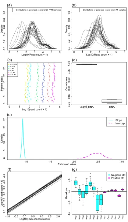
Figure B.1 in appendix plots raw read counts of six positive control probes vs. patient index for FFPE samples. It shows that on the un-transformed scale, the high count probes have high variance. This is a general property of count data generated from sampling dis-tributions, whose variance typically increases with the mean. Thus, we apply the commonly used log transformation to the raw counts; and to avoid 1 arising from zero counts, we add 1 to the observed counts before applying the logarithm.
The empirical distributions of the log10 transformed gene read count of FFPE vs FF samples are showed in Figure 2.1(a) and (b), respectively, in which each (density) curve corresponds to a patient sample and is plotted using log read counts of housekeeping and regular genes. It is obvious that the locations of the distributions of FFPE samples vary more dramatically than those of FF samples. This indicates the existence of heterogeneity in RNA degradation and fragmentation levels among the 28 FFPE tissue samples, contributing to individual sample effects in transcript abundance. This should be modeled, whenever possible, to enable comparison of gene expression levels between patients after removal of such technical artifacts.
Figure 2.1(c) plots log read counts of six positive control probes vs. patient index for FFPE samples. Compared with Figure B.1, we can see that the log transformation greatly stabilizes the count variance. Another noticeable observation is that the zig-zag patterns for the six probes are so similar, strongly indicating the existence of the lane effects.
Given a sample i, one would expect that the log transformed read count (sayYij) of any probe j has a monotonically increasing relationship with the corresponding RNA amount
(say Rij). Using positive controls whose RNA amounts are known and fixed over all i (i.e.,
Rij ⌘ Rj and Rjs are known), we can compute the correlation between Rij and Yij and that between Xij and Yij for each patient i, where Xij ⌘ logRij. Figure 2.1(d) shows two boxplots based on FFPE samples, one for the 28 correlations using log RNA amounts and the other for those using original RNA amounts. We can see that the correlations using log RNA amounts are much higher, with values very close to 1. Thus, a linear relationship between the log RNA amount Xij and log read count Yij seems to capture the underlying
Figure 2.1. Exploratory analysis of lung cancer data from xie et al. (Xie et al.,2017). Panels (a) and (b) show empirical distributions of log read counts based on housekeeping and regular genes for the 28 FFPE and FF samples, respectively. For FFPE samples, panel (c) plots log read counts of six positive controls (with different known RNA concentration amounts) vs. patient index; (d) compares the boxplot of correlations between log RNA amount and log read count with the boxplot of correlations between RNA amount and log read count; (e) shows empirical densities of patient-wise intercepts and slopes, and (f) overlays the 28 patient-patient-wise fitted lines of log read count vs log RNA amount, all estimated using data from positive controls; and panel (g) shows boxplots of residuals for the eight negative and six positive controls from fitting the linear trend (2.1) per
pattern well. More precisely, for each sample i, this can be described by
E(Yij|Xij =x, ai, bi) = ai+bix, (2.1)
where ai and bi are sample-specific regression coefficients.
Figure 2.1(e) shows the empirical densities of ais and bis; and 2.1(f) shows the linear trend (2.1) for each patient, all estimated using FFPE data from positive controls. The straight lines in Figure 2.1(f) are similar but apparently do not overlap. This suggests that the simplifying assumption ai ⌘a (or bi ⌘b) is not appropriate; but ais (or bis) share some commonality and so may come from the same distribution. From Figure 2.1(e), we can see that the two distributions are well apart with different spreads; and the Shapiro-Wilk test (Shapiro and Wilk,1965) suggests no gross departure from normality at the significance level 0.05for either distribution. Thus, it is plausible to assume that ais and bis are random and follow two separate normal distributions.
For every housekeeping or regular gene, the RNA amountRij reflects genej’s expression abundance in sample i, whose value is unknown. But for negative controls, Rij ⌘0 so that
Xij = 1, which is ill defined. To solve this issue, we add a small positive number so that Xij = log instead and (2.1) holds for negative controls as well. Both and Rijs are estimable. The intuition is that with the information from positive controls, we can pin down (ai, bi) for each sample so that with observed counts from negative controls, we can estimate , and with observed counts from housekeeping or regular genes, we can estimate
Rijs.
We use Pi=1
P
j2J (Yij aˆi)/ˆbi to obtain a rough estimate of log for FFPE samples, whereJ denotes the index set of negative controls, and ˆai andˆbi are estimated using data from positive controls as before. We then compute the residuals, i.e. deviations from the linear pattern (2.1), for each positive and negative control, and their boxplots are shown in Figure 2.1(g). Two interesting observations can be made here, which will be useful for the model construction in Section 2.2.3. First, negative controls tend to have much larger
deviations than positive controls; and their distributions tend to have much larger variability (hence wider spreads). Second, for each individual probe, the residuals are not randomly dis-tributed around zero: all the boxplots for positive controls are entirely above/below zero, and most boxplots for negative controls have 75% residuals or more above/below zero, indicating residuals are clustered by probes.
2.2.3. Proposed data model based on RCR
Letiindex (FFPE) patient samples, pindex positive controls, n index negative controls, h index housekeeping genes, and r index regular genes, for i = 1, . . . , I, p = 1, . . . , P, n = 1, . . . , N, h = 1, . . . , H, and r = 1, . . . , R, where I is the number of patients, P, N, H and R are the (prespecified) number of positive controls, negative controls, housekeeping
genes and regular genes in the NanoString nCounter platform, respectively.
Motivated by the analysis in Section 2.2, we set up a system of (hierarchical) linear regression models with random coefficients for the four different types of probes, in which the general linear relationship between the observed log read count and log RNA amount (either known or unknown) is assumed regardless of the probe type; and except for the observed log read counts, all the random components of the system are assumed to be independent. We begin with the model for the positive control class, given below:
Yip+=ai+biXp++d+p +e+ip, (2.2)
where Y+
ip is the logarithm of read count plus 1 of the pth positive control from the ith sample, X+
p represents the logarithm of the known RNA input amount (unit: f M) in the reaction system, and the superscript ’+’ indicates the membership of the positive control class. The ai and bi are the sample-specific random intercept and slope which may reflect the lane-by-lane variation. According to Figure 2.1(e)-(f), we may assume ais and bis be independent and identically distributed normal variables, respectively: ai
iid
⇠ N(µa, 2a) and
bi iid
pattern (2.1) (see Figure2.1(g)) and we assumed+
p ⇠N(0, d2). Finally,e+ip⇠N(0, e2)is the random error term, which reflects the remaining variability of the log observed count after taking into account the linear trend and the probe-specific deviation.
For the negative control class, the model is given by
Yin =ai+bic+dn +ein, (2.3)
where Yin is the logarithm of read count plus 1 of the nth negative control from the ith
sample, c ⌘ log is an unknown constant, the superscript ’-’ indicates the membership of the negative control class, and the other terms are defined similarly as in (2.2). As shown in Figure 2.1(g), the distributions of deviations (from the main linear pattern) for positive controls are very different from those for negative controls: from the centers (i.e., middle horizontal bars) of the boxplots, we can see dns vary more than d+ps; and from the widths of the boxplots, we can see eins vary much more than e+ips. Thus, we have to assume dn ⇠N(0, 2
d ) and ein ⇠N(0, e2 ), where the data suggest that d2 > 2d and e2 > e2. For the housekeeping gene class, the model is given by
Yih⇤ =ai+biXih⇤ +d⇤h+e⇤ih, (2.4)
whereX⇤
ihis the unknown log RNA amount of thehth housekeeping gene from sample i, the superscript ’*’ indicates the membership of the housekeeping gene class, and the other terms are defined similarly as before. Unlike positive or negative controls, Xih⇤ in (2.4) is random
by nature rather than being constant, which can be decomposed into a random term⇤
ih and a fixed term i, i.e., Xih⇤ = i+⇤ih. Here, i is a constant that reflects the individual effect of sample i in transcript abundance (e.g., patient-to-patient variation, variation in RNA
degradation and fragmentation levels of FFPE tissues, variation in the amount of input sample material, etc.), satisfyingPIi=1 i = 0; and⇤ih⇠N( ⇤h, 2⇤)reflecting the remaining
expression abundance after adjusting for the sample effect. Note that E( ¯X.h⇤) = ⇤h, where ¯
sample effects is and gene effects ⇤hs are both modeled as fixed effects instead of random effects. This is because for a specific sample, we are interested in recovering ⇤
ih from Xih⇤, rather than inferring the marginal distributions of is and ⇤hs.
For the regular gene class, the RNA amounts in different samples are unknown, too. So the model is set to be the same as that for the housekeeping gene class, but with a difference probe index r and no superscript (for notational brevity):
Yir =ai+biXir+dr+eir, (2.5)
where Xir = i+ir is the unknown log RNA amount of the rth regular gene from sample
i, and the definitions of ir, dr and eir are self-evident. Correspondingly, we assume ir ⇠
N( r, 2). Note that two separate variances, 2⇤ and 2, are needed for the housekeeping and regular genes, respectively. This is because expression levels of housekeeping genes are known to be more stable across samples, and so one would expect 2
⇤ < 2.
In the reaction system of the nCounter platform, negative controls have no known target and all detected binding signals should be from non-specific binding while positive controls, housekeeping and regular genes all have known targets, and so their working mechanisms may be similar. Thus, we assume d+
p, d⇤h, dr ⇠ N(0, d2) and e+ip, e⇤ih, eir ⇠N(0, 2e). We comment that for the housekeeping and regular genes, (2.4) and (2.5) are both hierarchical: the bottom layer involves a linear regression model with random coefficients, and the second layer (for the unknown log RNA amount) involves a two-way ANOVA model, where one factor represents the sample-specific effect i and the other factor represents the gene-specific effect that are related to ⇤
h or r. In addition, for all the four classes, since gene-specific deviations from the main linear trend (2.1) are allowed throughd+
p,dn,d⇤h anddr, the log read counts of the same gene from different samples (e.g., Yir and Yi0r) are correlated; meanwhile, the log read counts of the different genes from the same patient (e.g.,Yir and Yir0) are correlated, too, as they share the same random intercept ai and slopebi.