Data Mining and Automatic Quality Assurance of Survey Data

(1)

Autumn 2011

Bachelor Project for: Ledian Selimaj (081088)

Data Mining and Automatic Quality Assurance

of Survey Data

Abstract

Data mining is an emerging field in the computer science world, which stands in between the fields of statistics, machine learning and pattern recognition. Classification is one of the main tasks of data mining and its ultimate goal is to describe or predict certain unknown data into predefined categories based on knowledge acquired on data of the same type beforehand.

Programmatic quality checking of field survey data is difficult as it requires manual supervision to be able to identify and differentiate data trends. This paper attempts to explore the possibility to run various classifiers on field survey data and then use different techniques to build classification models to mimic manual supervision of data to programmatically check the quality of field survey data.

The choice of the right classifiers and model testing techniques are of crucial importance for the whole process as the main purpose is to ensure high reliability of the predictive classification models that will be used to predict the category where new and previously unknown data pertains. Emphasis is placed on picking and utilizing the best classifiers as well as to test with several manners and combine them for a classification task in order to provide more accurate results than just using one single algorithm, which might suffer from structural problems.

I accept that the report is available at the library of the department

Student: Ledian Selimaj Sign... Supervizor: ChengziChew Sign... Company: DHI

Coordinator: Hans ChristianPedersen Sign... Ext. Examiner: Jens DamgaardAndersen Sign...

(2)

(3)

This is to verify that:

• The entire material in this thesis report contains only my original work • All acknowledgments for the material referenced has been explicitly made

Ledian Selimaj January 2012

(4)

(5)

(6)

(7)

Acknowledgements

Not everything that counts can be counted, and not everything that can be counted counts (A. Einstein)

This bachelor thesis was done at DHI. All the material used for the study was provided by the DHI Data Center.

Special thanks to:

Chengzi Chew for his supervision and technical support Hans C. Pedersen for his supervision and encouragement

(10)

(11)

Chapter 1

Problem Formulation

This thesis attempts to explore the possibility to use data mining learning algorithms and tech-niques to perform quality assurance of field survey data by labeling the data as being correct or not. The data is gathered from numerous sensors in the stations that reside in particular sites in the Baltic Sea. The presence of incorrect data is due to some errors that might occur on the sensors that gather the data as well as some other external factors during data transmission from the stations to the data center. The central task is to derive conclusions on some of the best data mining techniques and algorithms that could be used for the quality assurance of the data. Certainly, in order to achieve this many tests should be performed and necessary analysis should be carried out on their results. Implementation of an application that would provide the needed data mining apparatuses to perform the tests is also a significant part of this thesis. The main issues to be solved in order to have a successful approach toward the problem solution are:

• Constructing data sets

Special attention is dedicated to constructing the proper data sets that would be inputs for the classifiers by ensuring that there is enough information for them to find the patterns underlying the data. However a proper analysis on the physical meaning of the data should be done in advance. The classification of wrong and right data is not trivial and a number of parameters should be included in the data sets in order to make the classification process easier and more accurate for the classifiers. The decision on what data to be included has to do with the correlation of the various physical parameters and necessary discussions on that matter should be done in accordance with the classifiers performances that run on these data.

• Using the best data mining practices

The data mining process of building and testing a classification model is done by following a specific protocol. There are several possibilities of using them, therefore a number of necessary tests should be done to pick the most reliable and safe technique both while

(12)

creating and testing a classifier. Reliability of the performance of the classifier model during testing is very important since that would be considered later when classifying unlabeled data by ensuring that the result of the classification would be as accurate as possible. • Selecting the best classifier

Judging about performance of a certain classifier for a given problem and compare it with others is always done with the aim of picking the best performing classifier. However this becomes complicated when the results of many classifiers are close to each other. Thus several measurements of the performance of each classifier should be considered to make a decision for the best one. Special measurements that show how good the particular classes are classified by the classifier get a special attention. There are also other techniques use to combine several classifiers together for making a single classification. A verification on how well does this technique improves as compared to the classification done by a single classifier needs to be done. The results of the use of some ensemble methods has shown to be promising in the data mining classification task. Thus a discussion on the degree that the ensemble classifiers might have over the ”primitive” once has to be verified through some tests.

(13)

Chapter 2

Introduction

This chapter presents the problem of this thesis from the business point of view. This is a real life problem and a solution might be offered by the use of data mining. A definition of data mining is stated and then a brief explanation on why and how data mining can be used to provide a reasonably solution for the problem introduced. Afterwards a data mining problem solving methodology is briefly explained following the objectives of the thesis as well as an outline of the following chapters.

2.1

Business understanding

Numerous hydrographical data is being transmitted from three large monitoring stations placed at different water depth in the Baltic Sea. These stations transmit data directly to a data handling center located in Denmark. It is the data center’s task to consolidate, continuously monitor, and ensure quality assurance and reliability of the transmitted data. The former is a difficult task to be done automatically since the judgment whether the data coming from the sensors is correct or not includes the evaluation and analysis of many parameters, their historical values, the time of the year when the data sample is taken and many others. Data mining classifiers could be of usage in this situation. They run on the data and construct classification models that can accomplish the required classification of the data, that is to classify (label) each instance of the data set to be either correct or not. So, data mining classification models might provide a convenient way to atomize the quality assurance process of the field survey data.

2.1.1 The problem

The data is coming from the sensors placed in the sea through a transmission to the data handling center. The raw data is stored in a database after some reallocation and calibration processes. Afterwards is the time for the automatic quality assurance (autoQA) to do some checks on the quality of the received data. After this post process has successfully finished the data is updated

(14)

in the database. The autoQA goes through the data, makes some check and assigns a flag to each of its instance depending on the result of the check. For example, if the data is ”bad” it is marked with 4, otherwise it is marked with 5 [17]. The value of the flag depends on the calculations and a bunch of checks performed on the values of each attribute of the data instances. The tests that need to be done in order to check the correctness of a data instance are:

-check if the value exceeds a predetermined threshold as its maximum value allowed -check if it goes below a predetermined threshold as its minimum value allowed

-check if its value is increased within a predetermined gradient in 1 measurement time step -check if its value is decreased within a predetermined gradient in 1 measurement time step -check if its value is repeated for a predetermined number of time steps

The automatic quality assurance process is followed by a manual quality assurance of data. Be-cause the autoQA filter lacks ”intelligence” and threshold values have been hardcoded, it makes wrong classification of ”good” and ”bad” data instances. Therefore a reviewer needs to manually go through the data and change the automatic quality assurance flags based on many standards and relations among the data. This process is very time consuming as well as expensive. A person needs to check every instance on the data sets and decide if the automatic quality assurance made a good or bad classification. Subsequently, the idea to automatize this process is raised. Such an automatic process will provide both faster processing as well as cheaper cost. Learning algorithms that perform similar checks as the review does manually can be used in this situation. Since the task at hand is a classification task, data mining classifiers offer a good chance to atomize the autoQA filtering.

2.1.2 Why data mining?

There are many different definitions on what data mining is but what is the core of all is that data mining is the process of automatically discovering useful information in large data repositories [1] . This useful information (or knowledge) is found as patterns on the data in different structures. By structure is meant that the patterns found are represented in an explicit form, for example a tree, a bunch of rules, decision tables etc. The power of these patterns is that the meaningful information found on some data can be applied to data that is previously unknown and used for classification predictions, which leads to some advantages, usually economic ones [2] . The benefits of having a classification done by a computer program are obviously greater as compared to for instance manual classification, which is quite impractical for large data sets. Classification is also one of the main tasks of data mining. Predictive classification models can be seen as functions that have the class value as their output and some explanatory variables as inputs. Practice has shown that applying the learned knowledge structures to new data can generate satisfactory results in their prediction [2] .

Quality assurance of field survey data is a typical classification task. The data that is meaningful and conveys right information can be labeled as being ”true” or ”false” otherwise. Therefore patterns for particular data can be retrieved from data set that are already manually classified

(15)

2.2. DATA MINING AS A PROCESS 7

as being true and false and can afterwards be used to classify new data with empty class values. Certainly, the level of accuracy depends on the classifier as well as on the information that the data sets that it runs on contain. Data mining offers various techniques on how to get more and more accurate predictions. The process of constructing as well as testing the models should be accomplished in a manner that ensures reliability of the predictions abilities of a particular classifier. Subsequently, by obtaining this reliability, the chances for success in future predictions on new data are high.

2.2

Data mining as a process

Data mining consists of a set of tools and algorithms that could be used for different business problems solutions. However what really matters is the analyzes and the knowledge provided by using it and all its facilities and tools in the right way, and in some structured manner. Therefore data mining should be viewed as a process.

The particular standard process used is the CRISP-DM framework: the Cross-Industry Standard Process for Data Mining. CRISP-DM demands that data mining be seen as an entire process [3] .

According to CRISP-DM methodology the lifecycle of a data mining project consist of six phases:

• Business understanding

This phase describes the problem from the business point of view and tries to understand the objectives and requirements of the problem. Afterwards the problem is converted to a data mining problem.

• Data understanding

It is crucial for a data mining project to understand the nature of the data that is going to be processed. Analyzes of the attributes should be done and all the necessary information should be included in the data set. It is also convenient to go through the data and check its quality, for example if there are missing values, redundant instances etc.

• Data preparation

After all relevant analyzes and cleaning of the data have been made in the preceding phase the final data set needs to be constructed. This data set will be the input for all the models that will be constructed and used.

• Model building

There are many different techniques for building models in data mining. The choice of the best one is always a priority so several parameter and techniques should be tried

(16)

After having several models constructed in various ways, proper analyzes should be done to search for the best performing model and the most successful techniques used for con-structing it. At the end of this analyzes only one model is chosen for the task

• Model deployment

The model chosen will be applied to previously unknown data. Even if the purpose of the picked model is to increase the knowledge gained from the data, it should properly be applied on that data, otherwise the result may not be that satisfactory

Figure 2.1: CRISP-Data Mining project methodology [16]

Picture 2.1depicts the entire process as explained above. As noticed from the picture, going back on the steps is necessary. For example in steps of Data understanding, Modeling, and Model evaluation it would be appropriate to go one step backward during the process in order to make necessary changes in case something went wrong on unexpected results were generated. This is important to ensure that the whole process is compact and coherent to have the best possible results.

2.3

Thesis Objectives

The main subject of the thesis is to explore the opportunity of applying data mining classifica-tion models for assuring quality assurance of field survey data. It examines what are the right procedures that should be followed in order to get satisfactory classification result and reliability

(17)

2.4. THESIS OUTLINE 9

for future usage on new data. It also concludes on which classifiers should be used to achieve the same goal. Other ways to combine and utilize these classifiers should be tested on their ability to increase the overall performance.

Special attention is dedicated on constructing data sets aiming to avoid any missing useful in-formation that would affect the classification model performances. In this context some effort is put to see how the changes on the data sets such as including additional auxiliary information affect the performances of the models.

This thesis introduces a customized application that offers a set of tools and classifiers to make it possible to experiment and derive conclusions on all the above mentioned topics. The classifiers and the data mining techniques are retrieved, customized and utilized from the Weka system [4]. All of these are used in the context of achieving the goal of making good use of data mining in solving the problem at hand. Therefore the application is called AutoQA Monitor. Different use cases and the requirement specifications for the application will be shown in appendixes B. Also, a summary of the its functionalities will be explained in Chapter6.

2.4

Thesis Outline

Following the data mining project methodology CRISP-DM introduced in subsection2.2the rest of this thesis report will be structured as follows:

Chapter 3

This chapter explains in details all the steps followed to build the data sets used during this thesis as well as the physical meaning of them. This is done by closely looking at the attributes of the data sets. Focus is put at the class attribute as well, that is the attribute used for classification of each data instance. It also makes an analyzes from the data mining (and statistics) of the data to have a good understanding of the data being processed as well as to explore the possibility to apply some preprocessing techniques to them before using as input for different classifiers.

Chapter 4

This chapter explains in depth the process of constructing data mining classification models. Firstly a general view of the whole process is explained and then a more specific explanation is shown for each step of the process. Several model construction and testing techniques are presented and contrasted with each other in accordance to the tests done to seek for the best ones to use. Moreover this chapter explains the classifier chosen for the task as well as presents some other existing classifiers which are not included or used in the AutoQA Monitor.

Chapter 5

This chapter explains which factors were considered determinant in picking the best classifiers and at the same time contrasting with others and judging on the decision. Several statistical metrics are used to compare different classifier models. Another discussion is made on whether to use one classification model or combine several with the goal of increasing the classification accuracy. A visualization tool for comparing the class predictions of a particular classifier included in AutoQA Monitor is shown. It can be used to see how good two different class values have been predicted by a classifier. Finally, a word about the prediction of data with unlabeled class attribute is

(18)

mentioned and the tools available in AutoQA Monitor are shown. Chapter 6

This chapter explains the development of the AutoQA Monitor data mining customized tool and how the Weka system libraries were integrated into it. It explains its functionalities in accordance with the requirement specifications and use cases built for it. A verification of the correctness of the software is also presented.

Chapter 7

This chapter shows the overall conclusions of the problem solution by stating each conclusion after the necessary tests and verifications were performed. It also tries to map each of the problems presented in Chapter1with the corresponding conclusions derived after all the defined tests were successfully accomplished. It then mentions some future improvements on this thesis goal or some improvements that the AutoQA Monitor might have.

(19)

Chapter 3

Examining and Understanding the Data

As already stated in Section2.2, one of steps of CRISP-DM is understanding the data that will be used to discover patterns on. A data set should be carefully analyzed before being used as an input into a machine learning algorithm (in this thesis those algorithms are the classifiers). This chapter describes one by one the physical meaning, the construction, and the analyzes done on the data sets. In order to have a good understanding of the data various statistical measures are calculated both on the continuous (numerical) data and certainly on the nominal values which will be the classified attribute of the data set after performing different classifiers on them. Also, this chapter demonstrates how the data sets were generated using a computer program. There will be two different types of data sets introduced and analyzed.

3.1

Implications of data sets

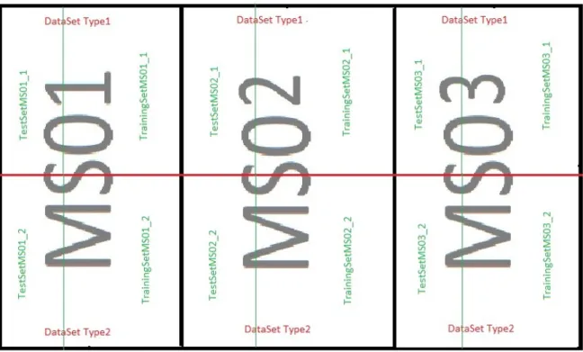
It is very important to explain the physical meaning of the data that is being used. The machine learning algorithms find patterns on data that contain some internal information. This section explains the attributes of the data sets and tries to define what they mean in another context, different from that of data mining. As already mentioned there are two types of data sets used, however they contain the same data. The second type has some modifications as compared to the first one. They will be explained later in this section.

The data set types consist of the following attributes respectively:

DateTime Turbidity WindSpeed WindDirection Depth Gradient ManualQA Table 3.1: Data set type 1 attributes

Those data sets that will be used for predictions on unlabeled data (new data) will have the same attributes but instead of ManualQA it will have PredictedQA. Before explaining all the

(20)

DateTime Turbidity WindSpeed WindDirection Depth Gradient NTU(t-1) NTU(t-2) NTU(t+1) NTU(t+2) ManualQA

Table 3.2: Data set type 2 attributes

attributes some general concepts are defined. Each data set consists of data for a particular station. There are overall data from three stations that are used for tests in this thesis. These stations are different in the sense that they are placed in different geographical locations. A station is a buoy containing a number of sensors placed on it that are collecting various data, for example salinity, turbidity, temperature etc. They are then transmitted to the data center via network. The focus of this thesis will be to provide some convenient and accurate ways to ensure the quality of turbidity data received from the stations.

A program was used to build the data sets. Since the data needed is in different files and the time stamps of their values are also different (even though close to each other), a merge is necessary to include all in one file. As already mentioned there are 3 stations, subsequently three main data sets will be constructed. However for the sake of testing and verifying how would the classifiers react to some changes on the data sets, another three data sets were created. The changes were made after some justifications to improve the accuracy of the classifiers as it will be shown again in the next chapter. Afterwards each of these six data sets is split into two parts in preserving the ratio 1:3 for one set and 2:3 for the other. The first will be used for testing during model testing and the second for training during model construction. So the total number of data sets constructed by this program is 12.

3.1.1 Attributes

DateTime is a timestamp of when each data instance is received. They are usually received in predefined time intervals that range from every 10 minutes to every hour. Continuous monitoring is the reason for getting data after the defined intervals. This is done to avoid losing necessary data in any case the sensors encounter an error of some type.

Turbidity

Turbidity is the amount of particulate matter that is suspended in water. Turbidity is measured by shining a light through the water and is reported in nephelometric turbidity units(NTU) [5] .

Turbidity makes the water look cloudy or opaque depending on the climate activity. During periods of normal wind speed and normal flow of the water, turbidities are low, usually less than 10 NTU. But during a rainstorm or a strong wind, particles from the surrounding land (rocks of just land) are washed into the water making it a muddy brown color, indicating water that has higher turbidity values. When it is also very strong wind, large waves are created in the sea, so the water flow is too high and the water volume moving is big as well, causing different particles from the bed of the sea to move in the upper direction and stir up with other existing particles, causing higher turbidities. Negative values of turbidity don’t

(21)

3.2. STATISTICS 13

exist and according the calibration of the sensors its value shouldn’t exceed 125. It can be inferred from the above description of turbidity why the values of two other attributes wind speed and wind direction. In case there are high values of wind speed, it is expected a high value of NTU and vice versa.

Wind Speedmeasures the wind speed in (m_/

s). The reason for including it in this data set is closely related to the turbidity values as explained above.

Wind Direction is used to check for objects on different directions from the position that the buoy is located. If for example it is close to the shore or there are some rocks in the surroundings then they might affect in an increase on the value of NTU. If nothing is on the surrounding then something else might have caused the increase in the NTU values or an error has occurred. This value is measured in degrees and has values ranging in the interval 0-360.

Depthis the water level value at which the sensors are placed in the field. Different NTU values are measured in different level, again according to the weather conditions. For example the surface might have lower level as compared to the lower ones in case there are high waves. Gradient is the slope of two data instances next to each other on their values of NTU over time. This is done because it is expected that the value of NTU should gradually decrease after reaching a high value, thus the gradient should have small, 0, even negative but not very big values.

ManualQAis the attribute of the classification of data done by a person after manually going through the data checking for incorrect NTU values received from the stations. True and False labels stand for correct and incorrect data instances.

In this context, the second data set type has four other attributes with two previous and two preceding values of NTUs. This is done to have more explicit information on the change of the values of NTU and to easily detect immediate changes of it.

3.2

Statistics

This section provides some analyzes on the data sets. In the context of getting to know the data it is important to perform some calculations over the data sets to examine the type of attributes, their value range, variance and so on. First the numerical attributes will be explained and then the class attribute. Afterward some correlation analyzes will be performed as well as some data quality checks on the data sets.

(22)

Figure 3.1: An overview of data sets used in this thesis

3.2.1 Numerical attributes

As already mentioned previously there are two types of data sets that will be examined and used for the data mining process.

The first data set type has the following numerical attributes: • Turbidity

• Wind Speed • Wind Direction • Depth

• Gradient

• Date Time: This attribute contains time stamps in the ”date” format as explained in [7] . These values are converted into doubles once uploaded to AutoQA Monitor (the same way Weka handles these type of values).

The following statistical summary will include this group of metrics for the data sets: MaxValuefinds the maximum value of the attribute

(23)

3.2. STATISTICS 15

MinValuefinds the minimum value of the attribute

Rangefinds the difference between Max and Min values. It is a measure of variability and it calculates the maximum spread on the data

Mean finds the mean of the values of an attribute. It is a measure of the location of data. if the data values is distributed in symmetric manner than this will be the middle value of the range of values the data contains

Median finds the median value of an attribute. It is the median value in between the higher and lower set of values. it is also a measure of location of the values of an attribute Standard deviationis a measure of spread of data.

DataSet Attribute Max Min Range Mean Median StDev

TrainingSetMS01-1 Turbidity 82.37 -0.241 82.611 0.85 0.603 0.968 WindSpeed 20.94 0.094 20.85 6.655 6.55 3.02 WindDirection 359.94 -11.34 371.3 193.7 211.95 94.34 Depth 17.2 1.2 16 6.65 9.6 5.13 Gradient 13109.76 -117328.32 130438.05 -0.036 0 269.06 TrainingSetMS02-1 Turbidity 65.189 -1.25 66.439 1.184 0.688 2.15 WindSpeed 20.007 0.003 19.98 6.509 6.45 2.948 WindDirection 359.964 -11.751 371.7 193.53 209.07 94.56 Depth 26.9 1.6 25.3 8.195 1.6 8.07 Gradient 8216.64 -9090.864 17307.5 1.007 69.357 1.7e10 TrainingSetMS03-1 Turbidity 82.37 -2.723 85.093 0.659 0.573 0.68 WindSpeed 20.63 0.004 20.59 7.03 6.97 3.147 WindDirection 359.869 -11.17 371.03 186.376 204.85 92.66 Depth 13.8 1.7 12.1 7.105 1.7 6.016 Gradient 13109.76 -117328.3 13207.25 -0.845 0 303.99 Table 3.3: Summary statistics of the training data sets

3.2.2 Class attribute

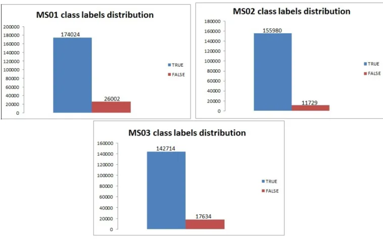
There is only one class attribute in all the data sets used. It is called the ManualQA and it can have only two categorical values (binary) : True and False. The following tables shows the distribution of each of the binary values of ManualQA attribute for each of the data sets in terms of frequency in order to have a better understanding on the ratio of data instances that are classified True and False.

As noticed from this table the class label ”False” is fewer in number as compared with ”True”. This is also the mode in all the data sets. Therefore it might be a challenge to correctly classify the ”False” data instances. It is also seen that the training and test sets for each station have

(24)

Station DataSetName FrequencyClassTrue FrequencyClassFalse MS01 TrainingSetMS01-1 0.87 0.13 MS01 TestSetMS01-1 0.88 0.12 MS02 TrainingSetMS02-1 0.93 0.07 MS02 TestSetMS02-1 0.94 0.06 MS03 TrainingSetMS03-1 0.89 0.11 MS03 TestSetMS03-1 0.88 0.12

Table 3.4: Frquencies of class labels for data sets of type 1

equal distribution of class values. The reason for doing this is explained in 4.2. The data sets of type 2 have the same distribution of class values thus they are not shown in the above table. Some histograms with the distribution of ”True” and ”False” class labels are shown in Figure 3.2.

Figure 3.2: Histograms showing the distribution of TRUE and FALSE class values for the data sets

(25)

3.3. ANALYSIS OF THE DATA 17

3.3

Analysis of the data

Before performing data mining model creation processes it is necessary to create a general idea of the data that is being used as well as apply some preprocessing techniques on it. This section shows some inspections done on the data sets to conclude on the quality of the data. Also a correlation analysis is done to find possible correlations between the attributes. Attribute selection and outlier analyzes are also included in this section.

3.3.1 Data quality

Data quality has a great impact on the success rate of the data mining algorithms. If wrong data is being input to the classifiers, the models generated won’t be so robust and will have poor performance on the classification tasks. The issues that will be considered regarding the data quality are:

• Missing values

Since the data sets were created using a program this issue is already handled. The data sets created have no missing value for each and every attribute they consist of.

• Duplicate values

For the same reason mentioned above, there are no duplicate values in the data set. A quick check for this would be to see if there is any time stamp which is identical. If so, the calculated gradient would be infinite, because the gradient is calculated using the following formula:

(turbidutyi−turbidityi−1)

(timei−timei−1)

(3.1) The gradient is calculated before data instances are randomized, thus it is done for every succeeding value. So, in case there will be any duplicated values of gradient there will be a division by 0 (infinity).

• Wrong values

As explained in the previous section, the attributes in the data sets have values that fall in a range of acceptable values. For instance ”turbidity” has values ranging from 0 to 125 NTU. Also, as seen from the statistics provided before for each attribute in every data set there are some negative values. Moreover the ”wind direction” attribute must contain values from 0 to 360.

Since every data on the data sets represents a real value retrieved from the stations in the field, taking those data out before training and building classification models would mean that those models will be too ”idealistic” and their performance on future classification tasks may suffer when it encounters these kind of data. However a test to verify how do these data impact the performance of the classification models can be done to make this verification.

(26)

3.3.2 Correlation analysis and attribute selection

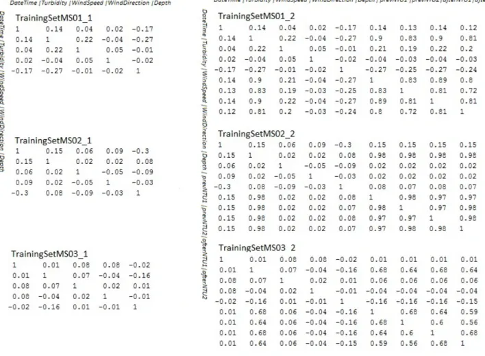
Correlation between two attributes with continuous values is a measure of the linear relationship between them. Its value is always in the range -1 to 1 [1]. A correlation of 1 means two attributes have a perfect positive linear relationship. That means that one can be build as a linear com-bination of the other in a linear equation of the form; y =k·x+b where x and y are the two attributes (for example represented as a vector of values ). Below will be shown the correlation matrices of 6 data sets, the training sets of the first and second types of data sets (since the test sets have the same attributes, subsequently the same data trends).

Figure 3.3: Correlation matrices for all training sets

The ”Gradient” attribute was removed from the calculations since it was generating many divisions with 0.

As notices from the matrices of training sets of type 1, the correlation coefficients are very close to 0, indicating a non existing correlation between the attributes. This fact means that the data

(27)

3.3. ANALYSIS OF THE DATA 19

set does not suffer from redundancy and all the attributes provided are necessary for model con-structions. This also implies that it is not possible to construct any of the attributes as a linear combination of another. Certainly every attribute can be constructed as a linear combination of all the other attributes by performing a principal component analysis, but this issue is out of the scope of this thesis.

On the other hand it can also be seen that in the training sets of type 2, the 4 attributes that contain the history ”turbidity” values are highly correlated with the ”turnidity” attribute since the coefficients have values like 0.9, 0.81, 0.83 and so on.

In case we perform an attribute selection on the different data sets (using CfsSubsetEval in Weka) the results would be:

Data Set Attributes

MS01-1, MS01-2 DateTime, Depth MS02-1 DateTime, Turbidity

MS02-2 DateTime, Turbidity, and afterNTU2 MS03-1, MS03-2 DateTime, Depth, Gradient

Table 3.5: Attribute selection for the training data sets

The attribute selection just keeps a subset of attributes that give most of the information on the data set and leaves out the rest of the attributes. So, the above presented output is a subset from the whole attributes of the data set based on correlation analysis between individ-ual attributes (features) that are not dependent on each other and don’t have redundant data. However, it should be noted that this is done mostly to reduce the processing time of model construction. The more attributes, the more time is required to build classification models. This approach will than be very convenient since it will reduce the running time of the algorithms by keeping at the same time most of the information from the previous data set. On the other hand such necessary information may be lost by taking out the other attributes. Also, even if the rest of the attributes (other than the ones presented in table 3.5) are omitted and the models are constructed without them, no significant change on the performance will be achieved. The attribute selection gives however some indications on which attributes are central and most important in the model construction phase.

3.3.3 Outliers

Outlier are data instances that are completely different from the rest of the data sets. As seen in the previous section, based on the statistics done on the continuous attributes, there are a number of data instances that have values which fall in a specific range around some value. Outliers are data instances that have values that don’t belong to any of this groups of values. Thus they

(28)

will impact the performance of the classifiers and confuse them during the classification process. Finding outliers is not trivial. Also, in the context of this thesis, the data being processed should be used as a whole since there is not a clear definition whether an instance that might be concluded to be an outlier from the data mining point of view it’s not from the physical meaning that the value represents. There are many techniques that can be used to detect outlies, as explained in [1] but they won’t be applied for this thesis.

(29)

Chapter 4

Model Creation

The next topic to explore according to CRISP-DM is the model building. This chapter depicts the process of model construction that was followed for the tests performed during this thesis and attempts to explain some decisions of the best methods to use in order to get good models. The goal is to get good and reliable results from these models. Also, a brief introduction to the nature of the classifiers used will be presented. Finally, some alternative classifiers will be mentioned.

4.1

Classification

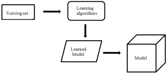
Data mining classification task is a two-step process. During the first step, model creation, a model or classifier is constructed to predict the class labels of each instance in the input data set. While in the second step (performing classification) this model can be applied for the same task to previously unknown data (new data). Classification is the task of assigning each data instance in a data set to predefined categories or labels. The models are constructed after a classifier has figured pattern on the data set that has each data instance already labeled. This is called the training set. As shown in [8], the concept is the same as a mathematical function Y = f(X) whereX is a set of attributes X = (x1, x2, ..., xn) and Y is a vector of labels (in this case True

and False)Y= (y1, y2, ..., yn) for each instance in the training set.

Figure 4.1: Data mining classification concept

(30)

4.1.1 Model creation process

The process of constructing models includes several steps. First the training set should be ready for usage (after doing all the necessary analysis previously) and then a classifier should be selected for building the model. Also, a testing technique should be chosen to view result of how good the model performs to classify the data in the training set. After the model has been built, it can be used for future classification tasks. This is explained in details in the next chapter. The AutoQA Monitor gives the possibility to select multiple classifiers to run on the training set. It also gives provides some of the most reliable model testing techniques that are used during model construction. Chapter6presents this functionalities in details. The classifiers can be of different internal structures. This means that the there are several ways to extract patters from the data. Decision trees and rules are two types of structures that will be explored further in this chapter.

Figure 4.2: Data mining model creation process

4.2

Testing techniques

The way to judge on whether a data mining model will reach the wanted success in classification tasks is to evaluate and examine its performance. There are different ways to achieve this but the protocol followed when building the models should be one that provides trusted results. The goal during model construction will be to create a model that will correctly classify as many data instances as possible when applied to the test sets that contain previously unseen instances. Another concern is that during model training phase the accuracy and error rate are generally too optimistic. This is because the same data is involved in training as well as testing. Subsequently the classifier can easily correctly classify and instance it used to build the model. In order to get a more realistic result the model should be tested on the test set that contains unknown data. These results would be a better measure of the performance of each classifier. This will be explained in details in the next chapter in the context of model evaluation and selection.

(31)

4.2. TESTING TECHNIQUES 23

On the other hand this section explains some of the best protocols used during model construction phase and derives a conclusion on which one is the best to use as supported by tests done using the AutoQA Monitor. The three techniques available are:

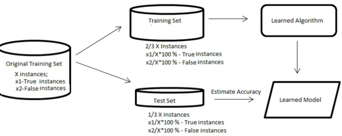
• Hold out In this approach the training set is partitioned into two disjoint sets usually in the ratio 1:3 for testing and the other 2:3 for training. The model is then constructed using the the data set portioned for training and is tested on the remaining data from the test set. So, the estimations on the accuracy of the model will be calculated on the test set, which has previously unseen instances for the model.

This method has however several drawbacks. First of all when using this accuracy assess-ment technique during model construction, fewer data instances are available for training, subsequently the model generated is not as good as it might have been if built including all the data. Also, the partition of the original training set may include most of the data instances with one of the class labels to only one of the sets. Therefore that particular class label will be overrepresented in one set and underrepresented in the other. Subsequently, the results may not be trusted.

In the implementation of hold out method in AutoQA Monitor another feature was added in the way the original data set is partitioned. The class labels in the training and test set after separation have the same ratio as in the data set before separation. This method is called stratification. It is done to ensure that both tests have the same distribution of class representatives as the original data set by including the right number of instances during the model construction and testing.

Figure 4.3: Hold out accuracy assessment method

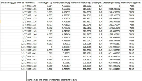
• Randomization Since the data sets that are being trained are time series data, there must be a way to make sure to include in the training and test set data from different years, months, days,and hours. Therefore another test method called randomization is implemented in AutoQA Monitor. A randomization algorithms is performed firstly to the

(32)

training set and then it is divided in percentage into training and test set. Usually (as in the hold out method) 66% of the data instances goes for training and the rest for testing. This technique suffers from the same issues as the hold out method. Also here there is no stratification done in order not to interfere in the randomization done according to dates. The data is partitioned directly after randomization.

Figure 4.4: A view of one of the data sets time stamp attribute

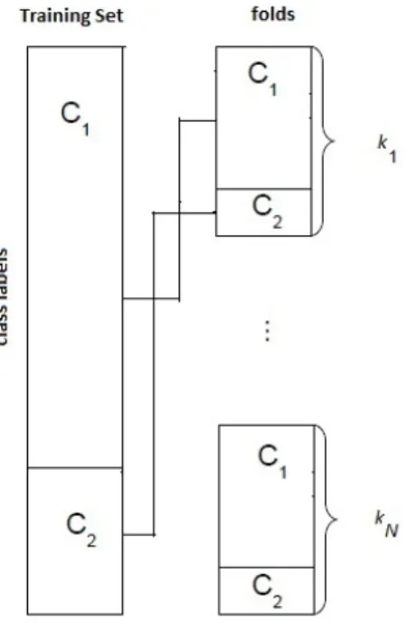
• Cross-validation Probably the simplest and most widely method used for estimating pre-diction error [6] . This technique is often used when the number of available data instances is not big enough. However it is also used to build a model that makes a good use of all the instance in the training set. The training set T is partitioned in k different parts and each of them is used exactly once for testing and once for training. So T= (k1,k2, ...,kN)

where k is the number of folds that the training set will be partitioned and N the number of instances in it. Each fold contains 1_k instances and each of them is stratified, so each of them contains the same ratio of instances with the class values as the original set. Af-terwards (k2,k3, ...,kN) are used as the training set and k1 as the test set. This process is

repeated for every fold. The total error is found by summing up all errors from each run or the accuracy is found as the average accuracy of all runs.

The decision on the value ofkis a topic for discussion but usually the 10-fold cross-validation is used, as well as 5-fold. [6]. A special case of this technique is the leave-one-out cross-validation when k=N. In this case each test set contains only one instance and the rest is the training set. This is beneficial in the sense that it utilizes the entire data set in the model construction by providing a better model. However this technique is very computa-tional expensive and is not very practical for relatively big data sets. An implementation

(33)

4.3. CLASSIFIERS 25

of leave-one-out cross-validation is also available in the AutoQA Monitor.

A schematic view of how the data is portioned and how the stratification is performed is shown in picture 4.5.

Figure 4.5: Partition of the training set ink-folds in the cross-validation method in a binary class problem

4.3

Classifiers

Choosing the right machine learning algorithms is one of the important decisions that needs to be taken when performing a data mining process. There are several alternatives that offer different ways to solve the classification problems. The difference consists of the particular manner that each of them find the patterns on the data. This chapter presents some of the algorithms that were included for usage in the AutoQA Monitor by giving a brief description on how they build the pattern on the data they are run, as well as providing some concrete examples from the patterns found on some of the data sets being studied on this thesis. At the end some other alternative classification algorithms different from the ones used for this thesis, are mentioned. All these algorithms will be called classifiers since their tasks are only concentrated in classification.

4.3.1 Trees

Classification using tree structures is done by the so called decision tree induction. In this tree the internal nodes are attributes and each outgoing edge is the outcome of test done on the values of these attributes. The leaf nodes contain class values. Certainly there is a root note that also

(34)

contains an attribute.

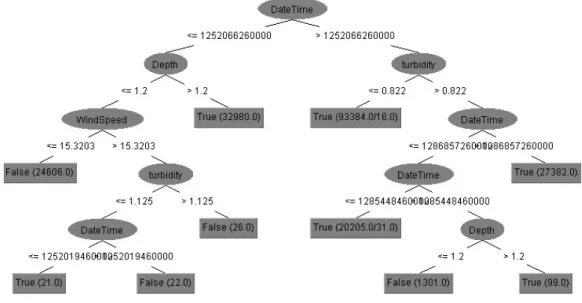
Decision trees are convenient to use in the sense that it does not require domain knowledge on the data [8].Moreover such a structure is quite intuitive and easy to grasp when applying new data on the tree. There are many types of machine learning algorithms (such as ID3) that use decision tree structures but in this thesis only J48 and RendomForest is used. An example of a decision tree constructed using J48 is shown in 4.6.

J48

It is the implementation of C4.5 in java (Weka)[2].This is an algorithm that is used for classifying continuous values attributes. The way it does this is by putting a threshold and splitting the set of data into two parts, one containing the values below the threshold and the other one above or equal to the threshold. This operation is performed recursively until the whole tree with purified leaves is constructed. The decision for the attributes to be involved in any node is done after calculating their information gain. The attributes with the highest information gain are chosen. This algorithm also handles missing values. The missing values are divided proportionally according to the rest of the data. It also offers the option of using pruning and validating the model in order to reduce the size of the tree of any of its branches if they are redundant and unnecessary. This contributes to make the process of building the models faster, but it can also have a negative effect on their performances since some of the tests done during the tree are lost.

Figure 4.6: A classification model of tree structure (J48)

It can be notices that all the leaves have the class values (True or False) and all the continuous attributes are split in two parts , being less or equal or higher than some number. This is a pruned

(35)

4.3. CLASSIFIERS 27

version of the decision tree for this particular model. The unpruned one is approximately double the size.

Random forest

This classifier is an ensemble method specifically designed for decision trees [1]. The basic idea is that it combines predictions made from many decision trees (this can can be specified manually) that are created on data from independent subsets of the training set. It is important to point out that all these subsets of data are stratified. Different alternatives are implemented to build the trees in this classifier. Some of them are: to select only some attributes as an input to the trees, or to select only a random feature with the best split for each node in the trees. After the trees has been generated and produced their predictions, a majority voting is performed on them to decide on the final outcome. It has been shown that this classifier can achieve satisfactory results compared to other ensemble techniques such as AdaBoost [1].

4.3.2 Rules

Rule-based classifiers use a collection of ”if ... then...” rules to extract and then build their clas-sification models. A set of rules is represented in a disjunctive form, meaning that many rules are ”AND-ed” together. The result of each set of rules is a class label. So each rule can be represented in the following way:

r1AN Dr2...AN Drk =⇒ yi

where the left side is the set of rules and the right side the class label.

Picture 4.7 shows the rules generated from PART on the same data set as the tree described above.

OneR

It is a type of association rule that involves just an attribute in the condition part. The criterion of the algorithm is to find that the attribute to be picked is the one that makes less error predictions. For each value of each attribute it counts how often does each class appear, finds the most frequent class and then it makes a rule out of it involving only that attribute and its value. Then it calculates the error rate of the rules and chooses the ones with smallest error rate. JRip

It is a widely used rule-based classifier that is mainly used for building models from data sets with imbalance class distribution. It chooses the majority class in two-class problems and learns the rules for the minority class. The algorithm performs basically two main steps, the rule growing stage when it builds rules on the data set until they are 100% accurate. Then it performs a pruning phase, where it incrementally prunes each rule of any final sequence in order to avoid very long

(36)

Figure 4.7: A classification model of rule based (PART)

and very specific rules. Finally, some additional optimization steps are done to determine whether some of the existing rules in the rule set can be replaced by better alternatives. The classification rule called JRip in WEKA was used.

PART

A PART model is a hybrid of rule-based classification and decision trees. First it uses an algorithm similar to that of J4.8. Then it takes the most accurate root-to-leaf paths and transforms these into classification rules that are used to build the model. This is done by both constructing and pruning the decision tree at the same time. The result will be a partial tree (or subtree) that cannot be simplified any more. [15] explains this algorithm in detail.

Decision table

This type of learning algorithm has as its core operation finding the right attributes to be included (attribute selection). This is done by doing cross-validation for different subsets of attributes and choosing the subset that performs the best. All the information is stored in the decision table. It is based on the simple idea that the output of the model will be a table. Then it’s a certain

(37)

4.3. CLASSIFIERS 29

judgment that decides on the classification task. It is based on those attributes that affect the decision the most. Those that don’t are left out of this decision. A detailed explanation of decision tables is made by [18].

4.3.3 Meta

This group of classifiers is called meta because they use another classifier as their base classifier to perform classification tasks. They are also named ensemble or combination techniques. The main idea is that they construct multiple models out of the training data and perform some aggregation of their classification to result into a single one. There are several ways of constructing these techniques, by manipulating the training data, the algorithms, the attributes, and the class labels. In general it has been shown that this type of classifiers tend to perform better than a single classifier as stated in [2] . Bagging and AdaBoost are the two algorithms used in this project. Random forest (which was explained in the subsection about trees) is also an ensemble technique but it only operates on decision trees.

Bagging

Bagging is an advanced data mining technique that was used in the experiments. It is also included as one of the choices of classifiers in the AutoQA Monitor. The ”Bagging” classification technique is implemented in Weka system and this was used to create the model. This technique repeatedly samples with replacement (that means that an instance used once is not omitted and can be picked again) from the data set, according to a uniform probability distribution and creates the co called bootstrap, which are subsets of data from the training set. The number of bootstraps is an input parameter that these classifier has. After creating the number of bootstraps it trains a base classifier on each of them. Afterward the test instance is assigned to the class that received the highest number of votes. Each model’s vote has the same weight during the voting. Bagging helps to reduce the errors associated with random fluctuations in the training data. This is also related to how good the base classifier performs, but bagging in general improves the performance of a base classifier which is not very stable. It must be emphasized that bagging does combination of only one type of base classifier at a time.

This can be used to increase the accuracy of a base classier that performs well on the training data by constructing bagging models with that base classifier. Several tests of this kind will be shown in the next chapter. [19] provides more details on this classifier.

AdaBoost

AdaBoost is an example of boosting ensemble technique. The same as in bagging, subsets of training data are created by sampling with replacement. Also this ensemble technique combines models of one base classifier type. It also uses voting schemes to combine predictions. Boosting runs also a number of times as specified by an input parameter. It has been shown that the more iteration the better and the lower the error on the training data is [2].

(38)

during the process of model construction. In this way it gives focus on classifying correctly a group of instances that are harder than others to classify. This can also result in model over fitting. Since a lot of focus is put on only a certain number of training instances, the model might not perform good when applied on new data. [20] presents more information on this classifier. Majority Voting

According to [9] one of the techniques that could be used as a combination of base classifiers is majority voting. This is more convenient in classification tasks where class labels are the target since it only involves counting each label. The predictions of each base classifier are retrieved and counted for each label. The label that gets most of the votes for each instance if chosen as the final predicted label. Each classifier included has equal vote weight, that is why [10] refers to majority voting as ”democracy”. [10] also shows that Majority Voting performs much better when the number of base classifiers is relatively big.

This technique would however be effected negatively in scenarios when one or some of the base classifiers performs really poor and the other satisfactory. Therefore a choice on the base classi-fiers should be made beforehand in order to ensure that the base classiclassi-fiers have an acceptable classification ability on the data sets.

In AutoQA Monitor Majority Voting is implemented in the way that is can operate after build-ing each individual base classifier on the data sets. Its implementation is adopted by Weka implementation of the meta classifier called ”Vote”.

Stacking

Stacking is another way to combine multiple models that have been learned for a classification task. It is an advanced techniques which gives each base classifier some kind of weight during the aggregation of the predictions from each of them. The idea is that the predictions from each base classifier (or level-0 classifiers) is all gathered into a new data set that will be used as an input for the meta-classifier (or level-1 classifier). This terminology was used by Wolpert, but [11] refers to it. It also refers to level-0 data and models and level-1 data and level-1 generalizer.

The issues raised when using this classifier are: what should the attributes of the level-1 data be; what level-1 generalizer (classifier) must to be used. Also a good choice of the level-0 classifiers is needed. During the tests and experiments that will be shown in 5.2.2 the level- 0 classifiers could be selected from all the above explained. As level-1 algorithm, a multi-response linear regression algorithm was used (MLR) as it was proved to be the best performing among other in [11]. The data set is converted intoI separate regression problems, whereI is the number of class values. The problem for classl has data instances with response equal to one for if they have class l and 0 otherwise. The input data set on this classifier will be the data set with the predictions from each classifier.

(39)

4.3. CLASSIFIERS 31

Figure 4.8: A schematic of how stacking works [11]

4.3.4 Alternative approaches

There are also other types of classifier in the data mining world but the above ones were chosen for usage and verification on their performance on the given task since their structure is much simpler to examine and since they are some of the most used classifiers.

Other types of classifier include:

• Instance-based classifiers Classification is done based on a number of similar instances with the test set. Therefore they don’t build a model for classification. They are also called lazy learners. Usually they are very computationally expensive.

• Artificial neural networksThis approach creates models using nodes and directed links between them in the same manner the human neural system works. Roughly speaking, a neural network is a set of connected input or output units in which each connection has a weight associated with it.During the learning phase, the network learns by adjusting the weights so as to be able to predict the correct class label of the input tuples.[8]

• Bayesian classifierThese classifier provide probability estimation that an instance belongs to a class label. These classifiers are usually time consuming, but quite robust to model over fitting. They are good in dealing with missing values and their performance is not affected by any irrelevant attributes in the data sets.

• Genetic algorithmsGenetic algorithms attempt to incorporate ideas of natural evolution. An initial population is created consisting of randomly generated rules. Afterwards, a population is created based on the fittest rules and the offspring of the rules. Offstring rules are constructed by applying the genetic operator like crossover and mutation. This process is repeated until the population evolves in such a way that each rule satisfies a predefined threshold of accuracy in classifying the individual members of a population. [8]

(40)

(41)

Chapter 5

Model Assessment and Selection

After having constructed a number of classification models, a decision should be made on the best one to use for classification on new data. According to CRISP-DM this step in the data mining process is called model evaluation. This chapter refers to model selection and assessment instead. Model selection is the choice of the best performing classifier and model assessment is the evaluation of a number of metrics on it after applied on new data set. All the decisions made on using the best classifiers and testing techniques will be supported by tests and experiments performed using AutoQA Monitor. A number of metrics to evaluate the performance of the classifiers will be explained as well.

5.1

Model assessment process

A good data mining classification model would be one that has high accuracy in predicting class labels on a data set. First of all a clear definition of accuracy needs to be done. Additionally, as credibility of the classifiers abilities is crucial, a reliable way to evaluate the models is necessary. This is the reason that the performance of each classifier will be determined on the capability of predictions on independent data sets, that are the test set.

In order to clarify how the evaluation is done, a clear distinction between the training error rate and the test error rate should be defined. The training error rate (as well as accuracy) are the values calculated during model constructing. They depend on the testing techniques that is used. If cross-validation is used, the estimation of the accuracy and error rate will be calculated only over the training set, whereas if hold out is used the evaluation will be done on the test set that is partitioned from the original training set (also called validation set). This evaluation is more reliable because it is done over unseen data. However, the number of instances on the validation set is small (only a third of the whole training set) and since the data has many similarities the results may be again too optimistic. The phenomenon of building models highly dependent on the training set is called model overfitting and is a disturbing problem in data mining. These models have high complexity due to the fact that they try to classify correctly as

(42)

many instances as possible from the training set, but perform poor on new data. For this purpose the experiments done for selecting the best models are done by evaluating the error rates and accuracy on previously unknown sets.

The picture below presents a schematic of the steps that are followed during the process of testing models. it is a continuation of the model creation process depicted in 4.2. Moreover, chapter 6 shows how this process is implemented in AutoQA Monitor.

Figure 5.1: Model testing process

5.2

Model selection

This section presents the metrics used to compare the accuracy of different classifiers. It also makes comparisons on different classifier structures and types. An analyzes between trees and rule based classifiers as well using combinations of classifiers versus using the best classifiers is done. All the conclusions will be inferred from various tests done to find the right answers from the above comparisons. These tests will be made in AutoQA Monitor and the result will be described and analyzed.

5.2.1 Measures of performance

A group of measures is to be verified after running a classifier on the training set. Primarily, a measure to show the general performance of the classifier is necessary. But the decision of the best performing classifier involves other measures as well. For instance an important aspect of the classifiers is how good it performs in each of the class labels. The problem at hand requires special attention to ”False” classified instances since they are scarcer than ”True” instances, as shown in the histograms in picture 3.2.

The following part of this subsection describes the measured that are available for analysis after testing a model (or models) in AutoQA Monitor:

Accuracyis a measure of the number of correctly classified instance of the test set. It is cal-culated by this formula:

(43)

5.2. MODEL SELECTION 35

Acc= T otalN umberof CorrectlyClassif iedInstances

T otalN umberof Instances (5.1) This measure will be calculated as a percentage. A high accuracy indicates an overall good performance of the classifier in the sense that many instances have been correctly classified. Error ratecalculates the fraction of incorrectly classified instances among all the instances of

the test set. It is calculated as follows:

ErrR= T otalN umberof IncorrectlyClassif iedInstances

T otalN umberof Instances (5.2) The goal is to get a very small error rate, as much as close to 0 as possible. That would mean that almost all instances are correctly classified. This is though just an ideal scenario. Root Mean Squared Error is a measure of error between the actual and predicted class labels. In general this measure is calculated for classifiers that predict number, but in the case of binary nominal class labels they are represented with 1 for ”True” and 0 for ”False”. The formula for its calculation is:

RMSE=

s Pd

i=1(yi−yi0)2

d (5.3)

where: y1 is the actual class label, andd is the total number of instances.

y10is the predicted class label for the i-th instance,

and d is the total number of instances.

Absolute MSis very similar toRMSE. Instead of the square root, it finds the absolute value of the sum of differences between predicted and actual class values, as shown in the formula below:

AbsoluteMS=

Pd

i=1|yi−yi0|

d (5.4)

where: y1 is the actual class label, andd is the total number of instances.

Confusion matrix is a very important measure that displays in a matrix the actual and predicted number of instances. It is a convenient way to have a proper view of how well a classifier did to classify each individual class label. where:

(44)

Predicted class Actual class

True False

True TP FN

False FP TN

Table 5.1: Confusion matrix for a binary class problem

• TP (true positive) This number indicates the ”True” instances classified correctly. • TN (true negative) This number indicates the ”False” instances classified correctly. • FN (false negative) This number indicates the ”True” instances misclassified as ”False”. • FP (false positive) This number indicates the ”False” instances misclassified as ”True”. The goal is to keep TP and TN as high as possible and the other two as close to 0 as possible. In this context TN (also called sensitivity), TP (also called sensitivity), FP, FN rates are also convenient measures to be considered.

TNR =TN /(TN+FP) TPR =TP /(TP+FN) FNR =FN /(TP+FN) FPR =FP /(TN+FP)

TNR and TPR are more important for inspection. A high number of TPR (its max value is 1) means that almost every ”True” instance was classified correctly. The same case is for TNR but for ”False” instances instead.

F-Measure is a metric that summaries two other metrics, precision and recall that are given below:

Precision(p) =TP /(TP+FP) Recall(r) = TP /(TP+FN)

So,p indicates how well did the classifier on the ”True” instances. If this metric is close to one means that most of the ”True” instances are classified correctly. It also tells that the number of FP is very low. On the other hand a high number ofr shows that the number of FN is low. The highest value these two metrics can have is 1 and that would mean perfect classification of ”True” labeled instances.

The F-measure is calculated as given below:

F= 2T P

2T P +F P +F N (5.5)

(45)

5.2. MODEL SELECTION 37

5.2.2 Tests and experiments

After carefully inspecting, analyzing, and understanding the data as well as the procedures to use data mining for pattern recognition, it is appropriate to test the level of success that can be reached by applying classification models is the data sets. The aim will be to detect a well performing classifier for each data set using the testing techniques, procedures, and measures as explained above. Attention will be put on exploring the ability of the classifiers structures used to make right predictions on the given data sets by the use of ensemble classifiers, visualization, and metrics on the classification for each class label. At the end of this subsection, an example of classification made on a data set with unlabeled class attribute will be presented.

Before showing the results, a schematic view of how the tests were performed is necessary to be pointed out. Picture5.2depicts the process followed for the tests accomplished:

Figure 5.2: Steps followed for the tests and experiments done for picking the best classifier for the data sets

Certainly, it should be mentioned that only the best performing classification model is found and presented in the tests. However there is another scenario presented in picture 5.3 where combination techniques are used and the results are a derived from the combination of several models.

The following, is a summary of the tests and experiments performed:

1. Tests to conclude on the best performing classifier for each data set

Table 5.2presents the summary of measures that were explained above in this chapter, for the best performing classifier on each data set. The primary criterion for selecting them was the accuracy. This tests are crucial for the purpose of this thesis. An analyzes of their results gives a general idea on how good do the selected classifiers on the data sets. As noticed, the overall performance is satisfactory. However specific observations like the classification for each class label, the performance of each classifier structure and other topics will be explained more in the remaining part of this subsection. The material for discussion will be some of the measures presented in table 5.2.

(46)

Measures MS01-1 MS01-2 MS02-1 MS02-2 MS03-1 MS03-2

Classifier PART PART OneR JRip OneR OneR

Accuracy 89.01% 90.33% 94.57% 95.32% 91.68% 91.74% Error Rate 0.1099 0.0967 0.0543 0.0468 0.0832 0.0826 RMSE 0.3314 0.3109 0.2331 0.2119 0.2884 0.2875 AbsoluteMS 0.1099 0.0967 0.0543 0.0502 0.0832 0.0826 numTP 90039 90039 76245 76855 68754 68797 numTN 1360 2716 5464 5502 6973 6975 numFN 0 0 4633 4023 5195 5152 numFP 11283 9927 63 25 1676 1674 FP rate 0 0 0.0573 0.0497 0.0703 0.0697 FN rate 0.8924 0.7852 0.0114 0.0045 0.1938 0.1935 TP Rate 1 1 0.9427 0.9503 0.9297 0.9303 TN Rate 0.1076 0.2148 0.9886 0.9955 0.8062 0.8065 F-Meassure(True) 0.941 0.9478 0.9701 0.9743 0.9524 0.9527 F-Meassure(False) 0.1942 0.3537 0.6994 0.7311 0.6699 0.6714

Table 5.2: Results of the best classifiers (built using 10-fold cross-validation) performances tested on the test set

2. Tests to decide on the best testing technique during model construction

This experiment aims to observe the results of the best performing classifiers using the hold-out testing technique introduces in 4.2and compare them with the 10-fold cross-validation results, which were shown in table5.2. The procedure of model construction and testing is the same as one explained earlier in this subsection.

As seen from the results, there is a slight difference in the accuracies of the classifiers. They appear to be lower than the 10-fold cross-validation results presented in table 5.2. The reason for this might be that the hold-out method uses less data for model construction than the 10-fold cross-validation, thus the models it generates can be less accurate as compared with the other technique. Since the data used to construct the models is smaller in number the chances are that some patterns on the data might be missed. Therefore the best testing technique used