Credit Risk Assessment Considering
Variations in Exposure:
Application to Commitment Lines
Shigeaki Fujiwara
Given the worldwide financial market confusion caused by the subprime mortgage problem and the increase in credit line contracts with relaxed covenants, there have been cases in which financial institutions are facing a demand to provide additional credit to securitized vehicles with height-ened liquidity and credit risks. These are typical examples demonstrating the importance of risk management considering variations in exposure. There are also calls for incorporation of future variations in exposure into the model for the Basel II advanced internal ratings-based approach. This paper adopts commitment lines as a credit provision with variable exposure and constructs a credit risk model whereby stochastic new borrowing demand is linked to changes in a firm’s asset value. Through simulations, the paper then considers the interdependence among expo-sure at default, probability of default, loss given default, expected loss, and unexpected loss. The paper also prepares a simple model for the covenants, and verifies the influence of the rigidness of covenants on expected loss and other risk factors.
Keywords: Commitment lines; Probability of default; Loss given default; Exposure at default; Expected loss; Unexpected loss
JEL Classification: G21, G32, G33
Deputy Director and Economist, Institute for Monetary and Economic Studies (currently, Director and Economist, Financial Systems and Bank Examination Department), Bank of Japan (E-mail: [email protected])
The author would like to thank Associate Professor Satoshi Yamashita of the Institute of Sta-tistical Mathematics and the staff of the Bank of Japan (BOJ) for their useful comments. Views expressed in this paper are those of the author, and do not necessarily reflect the official views of the BOJ.
I. Introduction
The subprime mortgage problem, which increased in severity during 2007, has trig-gered confusion in worldwide financial markets. It is also exerting diverse influences on financial institutions that do not directly hold such loans. For example, some types of financial vehicles, which invested in securitized subprime mortgages,1depended on asset-backed commercial paper (ABCP) for part of their fund-raising; as the ABCP has become difficult to roll over, these vehicles have made use of large sums of sup-plementary liquidity facilities (backup lines of credit) from certain European and U.S. banks. As a result of unexpected liquidity provision, banks’ balance sheets are suddenly expanding. In some cases, this strains the funding of the banks themselves, and the provision of credit to entities with heightened credit risk is resulting in massive losses. These cases illustrate just how important it is for financial institutions to manage risk stemming from variations in exposure beforehand.
There are also calls for the Basel II framework to mandate the evaluation of credit risk considering exposure variations. The first pillar of the Basel II accord requires the measurement of credit risk, market risk, and operational risk in the computation of capital adequacy for risk assets (Basel Committee on Banking Supervision [2005a, b]). Among these, banks must choose one of three methods for the measurement of credit risk: the standardized approach, the foundation internal ratings-based approach, or the advanced internal ratings-based approach. Banks that choose the advanced internal ratings-based approach must estimate the values of three factors which determine the amount of losses: probability of default (PD), loss given default (LGD), and exposure at default (EaD).
A great deal of research has already been conducted on PD and LGD, and progress has been achieved in the development of models. In contrast, for EaD almost all of the research substitutes exposure at the time when credit risk is evaluated, and only a few studies such as Moral (2006), Yamashita and Yoshiba (2007), and Kupiec (2007) address exposure variations through maturity.
Typical examples of exposure variation include (1) derivatives;2(2) bills, housing loans, and other instruments whose principal is repaid in installments (including pre-payments, etc.); (3) additional loans; and (4) commitment lines. Among these, addi-tional loans and commitment lines require a credit risk evaluation model that assumes changes in exposure because their risk is expected to increase via increases in expo-sure. Especially with commitment lines, banks cannot control their exposure, because they must passively provide new loans in response to firms’ execution for withdrawal rights obtained in compensation for commission fees. Accordingly, banks set covenants beforehand to prevent increases in exposure to firms with heightened credit risk. For covenants, banks use a combination of multiple conditions that can be observed and
1. The special purpose company (SPC) known as asset-backed commercial paper (ABCP) conduits is one ex-ample. ABCP conduits use CP and other relatively short-term fund-raising and invest in diverse securitized products. Banks provide these SPCs with securitized products, and provide supplementary liquidity facilities when issuing ABCP.
2. For example, the exposure in interest rate swaps is zero at the contract date, but the exposure then stochastically changes to positive or negative with subsequent changes in the yield curve: to be precise, the six-month forward rate curve.
easily verified, such as the worsening of a given financial variable beyond a given level. Recently there has been an increase in so-called “covenants light” contracts with comparatively loose waiver clauses in European and U.S. lending markets, and such lending has resulted in a stronger need for risk management.
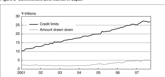
Figure 1 presents the credit limits and amount drawn down under commitment lines in Japan. The credit limits have consistently risen since 2001, and are now approaching ¥30 trillion. The drawn-down amount remained around ¥2 trillion through mid-2004 with little change, has been rising since then, and presently exceeds ¥5 trillion.
This paper considers commitment lines, whose market scale has expanded in recent years, and aims to present an example of a credit risk model that incorporates stochastic changes in exposure. The model also incorporates the effect of covenants on credit risks. The paper constructs a credit risk model whereby new loan demand changes stochastically in association with changes in a firm’s asset value, that is, a determinant factor of its PD, and evaluates the credit risk of commitment lines under conditions whereby there are correlations between EaD, PD, and LGD.
While more detailed verification based on the data of individual companies is of course necessary to confirm the appropriateness of the model and the parameter set-tings, the investigations focus on the following points using simple model settings and simulations through which cause-effect relations can easily be confirmed:
(1) What interdependence exists among EaD, PD, and LGD?
(2) What influence is consequently exerted on expected loss (EL) and unexpected loss (UL)?
(3) How does credit risk change with the rigidness of covenants, and what factors affect its optimal settings?
Figure 1 Commitment Line Market in Japan
Note: Figures cover city banks, trust banks, Saitama Resona Bank, Shinsei Bank, Aozora Bank, Regional Banks, and Regional Banks II.
Major findings and quantitative examinations are as follows.
(1) Credit risk tends to increase with exposure to the firm whose new loan demand rises when its asset value declines. Positive correlation between EaD and PD in the model describes this result.
(2) Covenants that prevent uncontrollable increases in exposure to poor performing firms are useful for limiting credit risk. In some cases, lax covenants can lead to greater losses, and this largely depends on the structure of how changes in a firm’s asset value lead to new loan demand.
(3) Consequently, verifying this structure is important for controlling credit risk when providing commitment lines and setting covenants.
(4) There is a covenants level that optimizes the trade-off between the increase in loan interest earnings and the increase in EL.
The remainder of this paper is structured as follows. Section II presents prior studies addressing exposure variations. Section III first presents an overview of commitment lines, and then attempts to create a model for stochastic loan demand via commitment lines, using the financial data of individual firms. By linking changes in a firm’s as-set value to changes in loan demand, a Merton-type structural model, which can be generally used to evaluate credit risk, is applied. Section IV evaluates the credit risk of commitment lines using a Monte Carlo simulation, and considers the optimal covenant settings for banks. Section V concludes the paper with a summary of the findings.
II. Prior Research on Exposure Variations
This chapter presents an overview of three research papers that address variations in exposure: Moral (2006), Yamashita and Yoshiba (2007), and Kupiec (2007).
A. Moral (2006)
Moral (2006) decomposes EaD: EaD
LEQ
(1)
where is the exposure at time,is the credit limit of the commitment line a bank sold at/before , and LEQ
is the percentage of the commitment line used from timeto default date/ relative to the unused commitment line at time. Moral (2006) attempts to estimate the unknown LEQ (loan equivalent), and attempts to derive EaD at time/. Specifically, he introduces the following three simplified methods:
1. Simple average of the observed values
We consider the LEQ over the coming year. First we collect data on default firms whose commitment lines have similar properties, such as the firm’s industry and stand-by or revolving type (see Section III for details), and then calculate the actually observed LEQ from the EaD at the default date and exposure one year prior to default. The LEQ value is estimated to minimize the sum of the squares of the error between the observed LEQ and the estimated value (in other words, the simple average of the observed LEQ is taken as the LEQ estimated value).
2. Weighted average of the observed values
While the above method treats all of the observed data equally, another approach is to weight the individual data by importance and then calculate the estimated value. For risk management, rather than knowing the future drawn-down amount by parties that are already close to full drawdown of their commitment line, it is more important to know the future drawdown by parties that still have a large amount unused. In this case, the weighted average of the LEQ values can be adopted as the estimated LEQ. One method for computing the weighted average is to use the square of the unused portion as the weight.
3. Minimization of the loss function
The damage from wrong risk management estimates differs in the cases of an over-estimate and an underover-estimate of the potential amounts of withdrawal. One way to ad-dress this is to incorporate a large penalty for underestimating the drawn-down amounts of commitment lines when estimating the LEQ. As an application example, Moral (2006) points to the estimation of minimum capital requirements, using an asymmet-rical evaluation function that assigns larger weights for underestimating the minimum capital requirements. Assuming that there is no estimation error for PD or LGD, the es-timation error for minimum capital requirements results solely from the EaD eses-timation error. The estimated LEQ is then found by minimizing the evaluation function.3
B. Yamashita and Yoshiba (2007)
Yamashita and Yoshiba (2007) examine the conditions where the bank supplies addi-tional loans to minimize the expected loss, and analytically evaluate how the new loan affects EL and UL.4
They assume that a firm’s asset value follows a geometric Brownian motion, and that banks can provide additional loans at specific points in time. Defaults by the firm occur when its asset value is less than its liabilities at loan maturity. Under these model settings, additional loans are made in two opposite cases. The first is the low asset value case in which the new loan contributes to a decline in PD. The second is the high asset value case in which the new loan contributes to an increase in interest income. The paper also notes that when additional loans are provided following the principle of minimizing EL, UL conversely rises, and highlights the undetected risk in the case of a bank decision made only on the expected value.
C. Kupiec (2007)
The Basel II formula for calculating minimum capital requirements in the first pillar takes EaD and LGD as given and makes the calculation using an asymptotic single risk factor (ASRF) model. On the other hand, empirical analyses show that PD, LGD, and EaD all grow larger during recessions.5 Kupiec (2007) attempts to model these positive correlations among PD, LGD, and EaD. Specifically, he uses latent variables
3. When there are estimation errors in PD or LGD, or when they are time variable, this is reflected in the value of the LEQ estimate. Estimation methods for EaD alone instead of the minimum capital requirements may be desirable to avert such a bias.
4. UL is defined as the expected loss under stress (SEL) minus EL. See Section IV for details.
5. EaD apparently increases during recessions because funds demand rises as cash flow worsens under poor busi-ness performance. One reason why LGD increases during recessions is that for loans with collateral the value of
to determine a firm’s asset value, LGD and EaD, using a common factor and individual factors that follow normal distributions. The setup establishes the correlations among PD, LGD, and EaD through the common factor. He then derives the analytical solution for the portfolio loss rate under these model settings. However, he does not explicitly incorporate the cause of the variation in EaD such as changes in firm funds demand into the model, and simply introduces changes in EaD as a stochastic process.
III. Commitment Lines and Funds Demand Model
A. Outline of Commitment Lines
The law concerning commitment line agreements6defines commitment lines as a “con-tract between a bank and its corporate clients, which legally obliges the bank to extend loans to the clients upon their request up to the amount that is agreed at the time of the contract within the term of validity that is also agreed at the time of the contract. The contract grants corporate clients the right to withdraw any time within the term of validity any amount up to the limit designated in the contract. In return for the commitment, the bank receives a commitment fee.”
More specifically, the characteristics of commitment line contracts can be summa-rized as follows.7
• Corporate clients can borrow funds at any time within the credit limit.
• Commitment lines can be categorized into two basic types: stand-by lines of credit used as a backup for emergency cases such as when it becomes difficult to issue CP, and revolving lines of credit for borrowings during normal times.
• The loan interest rate is stipulated at the time of the contract as a specific rate or as a spread over a reference rate such as the Tokyo Interbank Offered Rate (TIBOR) or the prime rate.
• Corporate clients pay a commitment fee on the credit line, or on the unused portion of the credit line.
• Banks sometimes set covenants in the contracts whereby they can refuse to pro-vide loans under commitment lines, mainly based on the deterioration in finan-cial conditions of the corporate clients such as the capital ratio and the interest coverage ratio.
B. Factors Determining Funds Demand
Many studies have examined commitment lines, including Campbell (1978) and Martin and Santomero (1997), partly because the commitment line market developed long ago in the United States. Those studies, however, are primarily concerned with the determi-nation of the fair value of commission fees and do not focus on modeling funds demand as the motivation for drawing down new loans. Therefore, the simple assumptions of
the collateral declines during recessions, resulting in a lower recovery rate upon default. Pykhtin (2003) notes that ignoring the correlation between PD and LGD results in an underestimation of the credit risk.
6. Operational since March 1999. With the implementation of this law, the use of commitment line contracts started to spread in Japan. This law stipulates that the commissions paid by borrowers under commitment line contracts are not regulated by the Interest Rate Restriction Law or the Capital Subscription Law.
funds demand models are unsuitable for the credit risk valuation model that considers the developments in EaD. Specifically, many of the earlier models cannot express the partial use of credit and drawdowns before maturity, because they make the simple assumption of full use of the commitment lines or no use at all, which is totally opposed to the concept of continuous stochastic changes in the EaD. To develop such a stochastic EaD, this paper begins by modeling new funds demand referring to the financial data of individual firms.
This paper focuses on changes in a firm’s asset value as a factor determining funds demand. In general, funds demand is expected to increase when a firm’s asset value is rising, and vice versa. However, a firm’s asset value may rise when the firm improves its financial position, for example, through a reduction in borrowings. It would be the case that a firm’s asset value may also rise using debt leverage contrary to the financial restructuring. Thus, the relationship between a firm’s asset value and funds demand may vary by company and across time. Moreover, funds demand does not necessarily decrease when a firm’s asset value declines. There may be cases where funds demand rises because of temporary cash flow tightening or backing out from a certain business line that incurs personnel restructuring costs. Because commitment lines are often con-tracted for working capital, it might be more appropriate to classify funds demand into funds for working capital and funds for capital investment; however, in this paper, for simplification we do not consider the use of funds.
We begin by examining the relationship between a firm’s asset value and funds demand using financial data on individual firms. First, we observe annual changes in total assets for a firm’s asset value and total liabilities for funds demand. Book values are used for both, for convenience. For total assets, we do not adjust for market value using market capitalization to calculate total assets as the sum of liabilities and share value. That approach would actually make the relationship between liabilities and total assets even more difficult to grasp, as share prices are strongly influenced by other domes-tic and foreign financial assets and especially by stock markets in other industrialized countries, which have been becoming increasingly linked in recent years.
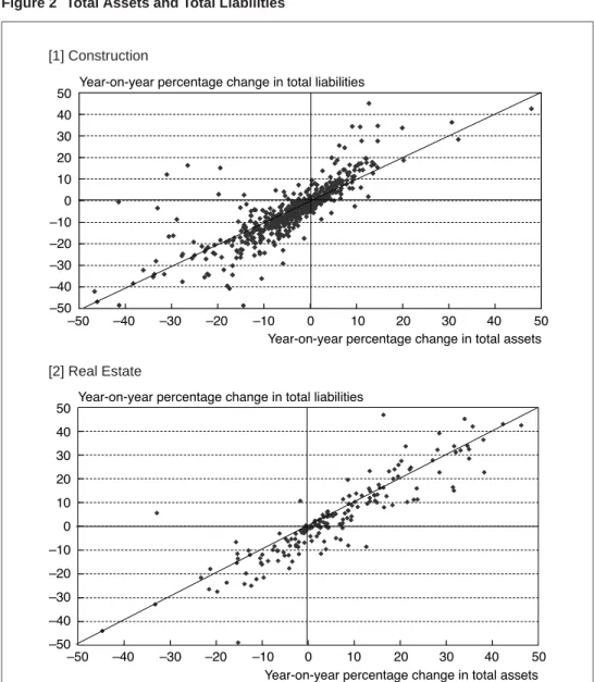
The data source is the Development Bank of Japan, with figures for each fiscal year from fiscal 1999 through fiscal 2004. The firms covered are those in the real estate and construction industries listed on the First Section of the Tokyo Stock Exchange. Firms in these industries have large changes in asset value and liabilities, and generally receive their financial support from banks. Figure 2 presents the annual percentage changes in total assets and total liabilities for each firm.
While Figure 2 indicates a strong positive correlation between the changes in total assets and liabilities, a considerable number of observations deviate significantly from the 45-degree line. The construction industry includes a substantial number of firms where liabilities increased while total assets declined, or where liabilities did not decline as much as total assets did. Conversely, liabilities of some firms below the 45-degree line in the third quadrant decreased more than total assets did. This might be a result of debt-equity swaps and write-offs of debt. Similar trends are observed in the real estate industry, but they are not as pronounced as in construction.
Figure 2 Total Assets and Total Liabilities
[1] Construction
[2] Real Estate
Note: A small number of observations could not be plotted within the graph boundaries.
Next, looking at the region where total assets increased, in many cases the increase was the result of greater debt leverage. That trend is observed especially in the con-struction industry. Conversely, there are some firms for which total assets increased by a smaller amount than their liabilities did.
C. Funds Demand Model
We proceed to develop the model with the assumptions that changes in a firm’s asset value influence funds demand, that banks are providing adequate commitment lines, and that additional funds demand over the existing loan amount will be filled using the commitment lines without contracting new loans. First we use a Merton-type structural model, that is, the standard credit risk model, to describe changes in a firm’s asset value. Specifically, a firm’s asset value follows the geometric Brownian motion shown in equation (2): (2) whereand
respectively represent the drift and the volatility in the firm’s asset value growth rate. The only liabilities are borrowings, and the liabilities at maturity will be the borrowings at the initial time plus the loans drawn on the commitment line. Default occurs if the firm’s asset value falls under total liabilities at maturity. In that case, net liabilities become the loss at default.
As for the timing of the drawdown, the period of time until maturity/ is divided intoparts, and the timing is expressed as , where /. The amount of each new loan via the commitment line, (
), is modeled as max Ratio (3) and & (4) where
is an indicator function with a value of one when the condition inside the bracketsis true, and a value of zero at all other times. Equation (4) for
repre-sents the linkage of the stochastic changes in funds demand to the changes in a firm’s asset value. We assume that funds demand is when a firm’s asset value rises and
when a firm’s asset value declines. Even when , liabilities may be trending up or down, so the time-trend term & is included. Furthermore,
is expressed as a stochastic process with the probability term
. represents volatility reflecting the uncertainty of funds demand and
is a random variable following a standard normal distribution. The error terms in equation (2) and equa-tion (4) are independent of each other. Equaequa-tion (3) includes a MAX funcequa-tion because of the assumption that loans via the commitment line are not repaid until maturity time /. While liabilities could actually be reduced through repayment prior to maturity, this assumption seems reasonable in the following sense. In general, loan terms seem to be determined in periods in which funding for a firm’s investments and business operations are stable. Unexpected increases in funding demand seem to be filled by the drawdown of the commitment line. Thus, the model in this paper targets credit risk valuation for a shorter period than the period reflecting long-term developments in loan amounts.
When new loan demand
occurs, the entire amount is borrowed as long as it is within the line limits and the covenants are not violated. When there is conflict with the covenants, the request for new drawdowns is refused. As for covenants, the interest coverage ratio and other financial indices are commonly used. In this paper the market-value basis capital ratio Ratio , asset value minus liabilitiesasset value, is adopted for the financial index referred to in covenants in order to incorporate the developments ininto the credit risk model. In short, commitment line loans are issued on demand only when the capital ratio exceeds .
The new loan makes a firm’s asset value and liabilities rise by the same amount. Thereafter, a firm’s asset value once again follows a geometric Brownian motion. Col-lateral is not considered, so the LGD becomesliabilities minus asset valueliabilities. Figure 3 presents an image of the model.
D. Determination of ,
Section C presented a model incorporating changes in a firm’s asset value into stochastic development in funds demand via a commitment line. In this section, we consider the specification of parameters and
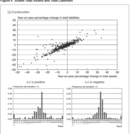
. The scatter diagram presented in Figure 4 uses the same data as in Figure 2, on an annual percentage change basis, and scales the data with total assets in fiscal . The histograms show the distribution of the slopes from the origin for these scaled annual percentage change data.
In the construction and the real estate industries, the distributions show a maximum slope of 1.0, regardless of whether is positive or negative. This leads to the hy-potheses that “the values of and
equal one, and the presence of the stochastic term in equation (4) results in a distribution around the slope one.” Looking at the slope distribution in detail, we see that whenis positive the maximum is one, but there
Figure 4 Scaled Total Assets and Total Liabilities
[1] Construction
is positive is negative
(continued on next page)
tends to be a long tail toward the negative, especially for the real estate industry. In contrast, whenis negative, the distribution is approximately symmetrical.
With reference to these observations, this paper sets the value of at one. On the other hand, the value of
is set as zero or negative under the assumption that “firms cannot restrain liabilities when their asset value is decreasing, and there are concerns that such firms may be forced to take on additional loans.” Such a hypothesis should properly be subjected to empirical analysis based on the individual company data with commitment line contracts. Because such data do not exist, this paper analyzes credit risk based on the above-stated hypothesis as the first step in the investigation of credit risk models for stochastic EaD.
Figure 4 (continued)
[2] Real Estate
is positive is negative
IV. Simulation Results
The simulation adopts the following simple settings to broadly reflect the characteris-tics of the credit risk model under which EaD depends on a firm’s asset value. First, we break down the continuous time model into a discrete time model with two periods and three points of time (present, six months later, and one year later), and assume that additional loan demand might occur six months later in a stochastic manner. The maturity dates for the liabilities at the initial time and for the loans drawn down on the commitment line are all one year later. We now proceed to calculate the values of PD, ELGD (expected LGD), EL, and UL through a Monte Carlo simulation under the above assumptions.
Before conducting the simulation, we set values for the parameters other than and
in equations (2) and (4), initial asset value (
using annual data from 1979 to 2006 for nonfinancial corporations under the Flow of Funds Statistics. First, we set and .based on the average capital ratio throughout the full period. The time series of this ratio generally shows fluctuation within the range of 20 percent–50 percent. We do not assume any specific scenario on the current condition in the ratio such as heightened debt leverage, so average values are used. Next, for the parameters in equation (2), we compute the average and variance of the annual ratio series for total assets and set the values at "percent,
percent. Finally for the parameters in equation (4), we scale the 1979 liabilities at 70 and set the values at& ,
.based on the average and variance of the liabilities annual difference series.
Under these parameter settings, however, the one-year PD becomes extremely low at 0.003 percent.8 Because the model characteristics can be interpreted more easily from the simulation results, we assume an enterprise with a somewhat high PD and set
at 20 percent higher than the original one of 10 percent. The values of the other parameters remain as stated above. With these settings, the PD becomes 2.7 percent, which generally corresponds to PDs for firms with a BB bond rating.
The credit limit on the commitment line is set at 20, and interest earnings for the bank are not considered in the credit risk analysis. The simulation is conducted 200,000 times to stabilize the calculation results.
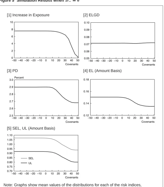
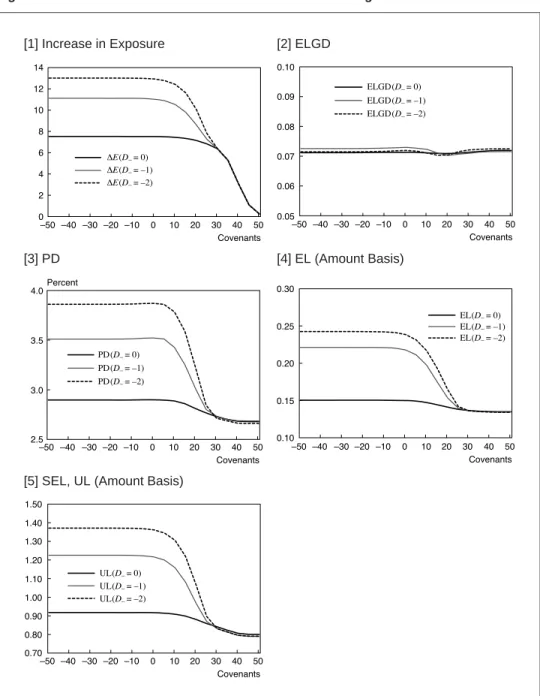
A. Case When
First we examine the case where the value of parameter
is zero. Figure 5 shows the simulation results for the expected value of the new loan amount, PD, ELGD, EL, and UL. The horizontal axis of the graph shows the measurement for the covenants, that is, the capital ratio (in percent).9
UL is calculated as follows. We assume a single-factor Merton model10under the as-sumption that the bank’s credit portfolio is well diversified; in other words, the amount of credit to any given borrower is sufficiently small in the overall portfolio. UL is calculated by subtracting the value of EL from the value of EL under stress (stressed EL), hereafter, SEL. We also assume a confidence level of 99.9 percent for the common factor under stress, with
/!
percent. The correlation between the common factor and a firm’s asset value is
.
11
In Figure 5, the covenants are assumed to be between"and 50. Covenant values of around the initial capital ratio of 30 percent or a bit lower are considered realistic. Despite this, we boldly set the covenants over a wide range for the following reasons. First, negative values, that is, capital deficits, are considered because the model does not consider default prior to the loan maturity during which firms may fall into negative net worth. Covenants above 30 percent are also considered to have the effect of setting strict covenants in cases when the bank does not allow further declines in a firm’s asset value
8. On a global basis, this is around the level of PD for corporate bonds with a rating of AA.
9. In this paper, covenants refer to whether or not the capital ratio is less than. For simplification, hereafteris referred to as “the covenants.”
10. See, for example, Yamashita and Yoshiba (2007) for the single-factor Merton models and the definition of UL. 11. Under the Basel II credit risk measurement for loans to nonfinancial corporations, parameter must be set at
Figure 5 Simulation Results When
[1] Increase in Exposure [2] ELGD
[3] PD [4] EL (Amount Basis)
[5] SEL, UL (Amount Basis)
Note: Graphs show mean values of the distributions for each of the risk indices, conducting 200,000 simulations.
with high credit risk or other more extreme cases when the banks provide a commitment line with a high commission, in expectation of an increase in the firm’s capital.
Next, we explain the changes in each risk parameter. We review the simulation results in the three broad categories of covenants levels: (1) the standard setting range of 0 percent–30 percent; (2) a very loose setting of 0 percent or less; and (3) a strict setting of 30 percent and above.
1. Increases in exposure
a. 0 percent–30 percent
The expected value of the increase in exposure is more than six and less than eight, and the liabilities increase by about 10 percent from their initial value of 70. The increase is more or less constant at a level less than 10 percent of covenants, indicating that the existence of the covenants does not restrict the increase in exposure in the range.
b. 0 percent or less
The covenants are not a constraint, and the new loan demand is just below eight. The new exposure figure depends on the probability of improvement in a firm’s asset value through equation (4) with
.
c. 30 percent and above
Because there are a large number of cases in the simulation where the covenants pre-vent new loan withdrawal, the mean increase in exposure declines as the covenants become strict.
2. Changes in PD
Under Merton-type structural models, the liability ratio determines PD. In other words, PD rises as debt leverage is utilized. This can be explained with equations as follows.
Just before the commitment line loan is drawn down, the firm’s asset value is, the liabilities are, and the period until maturity is/. PD is given by
PD ! / ln / (5) where!is a distribution function of a normal distribution. It is clear that when the other parameters in equation (5) are fixed, PD is determined by the liability ratio.
We now consider the influence of the new loan on PD. When the amount of the new loan is, the PD just after the loan is drawn becomes
PD ! / ln / (6)
This shows that PD rises (falls) because of the commitment line loan when the liability ratiorises (falls) from. Regardless of the amount of the commitment line loan, the liability ratio will increase whenever the loan is drawn in the case of net positive assets ( ), and decrease whenever the loan is drawn in the case of excess debt ( "). We now examine the changes in PD among different covenants levels.
a. 0 percent–30 percent
In the case of net assets, new loans always raise PD, but borrowing is restricted as the covenants become more severe. For that reason, PD is a decreasing function of the covenants level.
b. 0 percent or less
PD remains more or less constant at 2.9 percent. In a theoretical sense, (1) in the case of excess debt, commitment line loans reduce PD, and (2) making the covenants more se-vere weakens this effect, so PD is an increasing function of the covenants level, opposite
to Section IV.A.2.a. As discussed above in the examination of exposure, however, the covenants are not a binding condition for new loan withdrawal, so the effect of (2) is extremely small, and in Figure 5 PD is observed to be essentially flat.
c. 30 percent and above
Because the severe covenants restrict loan withdrawal, PD declines following the above-mentioned effect and ultimately converges to 2.7 percent when no new loans are made.
3. Changes in ELGD
ELGD remains constant at 0.07 regardless of the covenants level. Because ELGD has a low sensitivity to the amount of new loans, this has almost no influence on ELGD, even if new loans are restricted by covenants. An intuitive explanation is as follows. ELGD is calculated as the conditional expected value
. Here ,
respectively represent the firm’s asset value and the liabilities at maturity, and the
distribution determines ELGD. The
distribution in logarithmic form for the new loan amount ofis given by
ln ln / / (7)
Because ln has little sensitivity to and the ln
distribution is not influenced significantly by , ELGD remains essentially con-stant regardless of the covenants level. An explanation using differential calculations is presented in the Appendix.
4. Changes in EL
EL is approximately equal to the product of EaD, PD, and ELGD. Because ELGD is essentially constant as stated above, the change in EL is roughly explained by the changes in EaD and PD. However, to be precise, because all three variables follow distributions with correlations in the credit risk model, EL is not actually determined as the product of EaD, PD, and ELGD. Thus, to calculate EL, we calculate the expected loss through the simulation. While it is inappropriate to interpret EL as the product of the three variables, that approach is adopted here so that the interpretation is easy.
a. 0 percent–30 percent
EL gradually declines, mostly from the decline in PD. The effect of the decrease in EaD also contributes to the decline in EL.
b. 0 percent or less
Because EaD and PD are essentially constant, EL also remains constant at around 0.15.
c. 30 percent and above
The decline in EL is even gentler than that for Section IV.A.4.a. This is because while EaD suddenly declines, the decline in PD is limited. PD influences EL via existing exposure as well as new loan exposure. Ultimately, EL converges to 0.12 when no new loans are made.
5. Changes in SEL
a. 0 percent–30 percent
SEL is a decreasing function of the covenants. This is because if exposure is restrained by the covenants during the loan term period, SEL can be reduced even if a stress event occurs at maturity. SEL declines by 0.1 from covenants 0 percent to 30 percent. This
is largely greater than the 0.01 decline in EL, demonstrating that the covenants have a greater effect on SEL than on EL.
b. 0 percent or less
Because the increase in exposure and PD are essentially constant, SEL is also flat. Be-cause the covenants do not restrict an increase in exposure, SEL takes a maximum value.
c. 30 percent and above
Similar to EL, the size of the decline in SEL is gradual compared with Section IV.A.5.a. Furthermore, the area where the curve is convex is further to the right compared with EL. This is because the decline in EaD has a stronger influence on SEL than on EL. Ultimately SEL converges to 0.95 when there are no new loans.
As for UL (i.e., SELEL), because the variations in EL are less than those in SEL, UL has essentially the same shape as SEL.
B. Cases Where Is
or
Thus far, we have assumed that
, where no loan demand arises from declines in a firm’s asset value. We now investigate the changes in risk when
is
or,
assuming “increased borrowings following a decline in a firm’s asset value,” which poses higher risk to banks. Here, the settings of all the parameters other than
are left unchanged to observe the influence from changes in
. Figure 6 presents the simulation results.
1. Increases in exposure
When
is decreased from zero to
to, the increase in exposure rises because greater funds demand arises when a firm’s asset value declines. In the case of no upper limit to the commitment line, the increase in exposure becomes a linear function of
from the settings of equation (4). In Figure 6, on the other hand, the increase in the case of
’s shifts from
to is less than in the case from zero to. This is because in the simulation there are cases where new loans are restricted by the limit of the commitment line, and this reduces the average EaD.
When the covenants are set within the range of 0 percent–30 percent, the area where the increase in exposure begins to decelerate is around 20 percent when
is zero and around 0 percent when
is
. This indicates that when
and the covenants are loose, there is a large risk that the bank will not be able to restrain increased new loan demand. In contrast, when the covenants level approaches 30 percent exposure is almost the same regardless of the value of
, because the loan demand is suppressed by the covenants when a firm’s asset value declines. This shows that the relationship between covenants and increases in exposure can change greatly depending on the value of
, and suggests the importance of setting the covenants at an appropriate level.
2. Changes in PD
PD rises as
becomes smaller. The maximum differential of PDs between zero and
for
is nearly 1 percent. PD grows larger as
declines for the following reasons. New loan demand arises irrespective of whether a firm’s asset value increases or decreases six months later, but firms hold positive net assets in many cases. In this case, the liabilities ratio that determines PD rises along with the increase in new loans. As the negative value of
declines, the increases in the new loan and the liabilities ratio become greater. For that reason, PD rises because of declines in .
Figure 6 Simulation Results When the Value of Is Changed
[1] Increase in Exposure [2] ELGD
[3] PD [4] EL (Amount Basis)
[5] SEL, UL (Amount Basis)
When
is
or, PD suddenly rises as the covenants level decreases from 20 percent to 0 percent. Because EaD and PD have a strong positive correlation under a relaxed covenants setting, credit risk increases significantly. When the covenants are set higher than around 25 percent, however, PD becomes constant regardless of the value of
because an increase in exposure due to a decline in the firm’s asset value is restricted.
3. Changes in ELGD
ELGD remains nearly constant at 0.07 regardless of the value of
and the covenants. When the covenants are lax, intuitively ELGD would be expected to rise when large funds demand arises from declines in a firm’s asset value. However, as long as the assumptions that assets and liabilities rise equally from new loans and that the geo-metric Brownian motion parameter in equation (2) remains constant hold true, under the framework of the Merton-type structural model, ELGD is barely influenced by the covenants setting, similar to the case of when
. (See the Appendix for the reasoning.) The gap between simulation results and intuition suggests the possibility that these two assumptions may not hold.12
4. Changes in EL and UL
When the covenants are 30 percent or less, EaD and PD both rise from the decline in
, and thus EL and UL both increase significantly. In particular, UL more easily rises because SEL expands nonlinearly against the change in
. In Figure 6, SEL is only restricted because the limit of the commitment line is set at 20, and there is great potential credit risk under easy commitment line provision and lax covenants especially when
is negative.
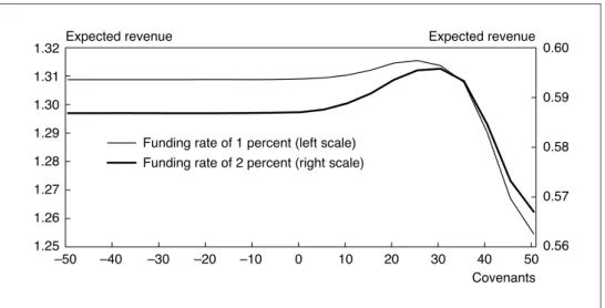
C. Optimal Covenants Setting
Up to this point, because the analysis has assumed no loan interest income, banks are able to reduce EL (always positive) by setting strict covenants. When interest earnings are considered for valuation of expected loss, however, another argument emerges; the optimal covenants level exists to maximize the total return composed of (1) higher interest earnings from the increase in loan amount and (2) higher expected loss at default because of the increase in loan amount. In this section, we examine this trade-off assuming that banks act to maximize their expected revenues including the expected loss.13
We now examine the optimal covenants level using simulations. The simulation settings are as follows. Banks provide new loans at a previously determined interest rate,. The bank’s funding cost is,
. The initial liability amount
and the new loan amount are stated at face value. In other words, the amounts that the firm actually borrows are discounted by lending rates.14 The simulation parameter settings are the same as for the case
, and, is set at 3 percent. Simulations are conducted for the two cases when,
is 1 percent and 2 percent.
12. For example, even when a firm has worsening performance, at the moment of new loan withdrawal, it remains as cash in the firm’s balance sheet. Consequently, the assumption that assets and liabilities rise equally when new loans are drawn is feasible. In reality, however, it is entirely possible that the asset may deteriorate from the moment this cash is used for the firm’s activities. In that case, the firm’s asset value does not increase by the amount of the new loan. Then, ELGD increases because the numerator of in equation (7) decreases.
Over a somewhat longer time frame, it is also possible that the cash borrowed by firms with worsened performance may not be used effectively. In that case, the growth rate of the firm’s asset value,, may be said to have declined during the period. Thus, a possible approach to avert this kind of problem is to setas a function of the firm’s asset value.
13. Another approach would be to consider the profit risk trade-off for risk calculated using UL. For simplification, we assume risk-neutral banks.
14. These settings are to simplify the expression of revenues as defined in equation (8), and whether the funding amount is measured on a discounted basis or face value basis is an unimportant issue.
Figure 7 Optimal Covenants
Under the above settings, the expected revenuesare
(8) where # is the time from the drawdown of the commitment line to maturity. The simulation results are presented in Figure 7.
The expected revenues are positive when there is a spread to some extent between the lending rate and funding rate. The optimal covenants level is 30 percent when the funding rate is 2 percent and 25 percent when the funding rate is 1 percent, which suggests that optimal covenants are not lower than 30 percent of the initial capital ratio. When the funding rate is 1 percent, the volume effect of the increased exposure exceeds the negative influence of increased credit risk, and therefore the optimal covenants value becomes smaller than in the case of the 2 percent funding rate.
V. Summary
This paper has constructed a credit risk model for stochastic changes in exposure and applied it to evaluate credit risk of commitment lines. Loans under commitment lines make it difficult for banks to manage risk appropriately, once such contracts are con-cluded and firms have an option to withdraw new loans. For that reason, the covenant conditions are important for risk management. We consider a model in which EaD, PD, and ELGD are mutually interdependent and a firm’s funds demand is explicitly linked to changes in its asset value. We apply the model to commitment lines, and calculate EL, UL, and other risk measurements. We also assume various degrees of covenants from relaxed to severe to examine the changes in EaD, PD, ELGD, EL, and UL and investigate their interdependence in simulations.
The following points were verified quantitatively through the simulations.
(1) Credit risk tends to increase with exposure to the firm whose new loan demand rises when its asset value declines. A positive correlation between EaD and PD in the model describes this result.
(2) Covenants that prevent uncontrollable increases in exposure to poor performing firms are useful for limiting credit risk. In some cases, lax covenants can lead to greater losses, and this largely depends on the structure of how changes in a firm’s asset value lead to new loan demand.
(3) Consequently, verifying this structure is important for controlling credit risk when providing commitment lines and setting covenants.
(4) There is a covenants level that optimizes the trade-off between the increase in loan interest earnings and the increase in EL.
Because individual companies’ commitment line data are not available, the exami-nation of the suitability of the model and parameter settings in this paper is insufficient. Moreover, this paper adopts several simplified assumptions to understand the property of the model that generates mutual dependence among EaD, PD, and LGD. The fol-lowing types of model extensions could be considered. These are left as future issues, along with the verification on the model based on empirical data.
(1) The funds demand model sets and
as constants, but it would enhance model applicability to make these parameters either functions of the firm’s asset value or stochastic variables.
(2) The model assumes that new loan demand always occurs at a specific point, but the timing and the presence or absence of loan demand could also be incorporated into the model.
(3) The model could accommodate funds prepayment prior to maturity instead of having all refunded at maturity.
(4) Funds demand is given as exogenous, but the model could be extended to make it an endogenous variable, for example, assuming the demand is determined to maximize shareholder value.
APPENDIX: CHANGES IN ELGD FROM COMMITMENT LINE LOANS
The ELGD for a new loan with a face value of is given by the following equation:ELGD ! exp/! / ! (A.1) where / ln /
We now calculate the first derivative to examine the sensitivity of ELGD to the amount of the new loan with a face value of :
$ELGD $ ! !exp/! / ! ! exp/! / ! (A.2)
The numerator of equation (A.2) is modified as follows:
! exp/!! / ! exp/! / ! / exp/!! / exp/!! / ! / exp/! / / exp/!! / / !exp/! / (A.3) whereis the density function of the standard normal distribution.
From equation (A.3), the denominator of$ELGD$ is far larger than the numer-ator, so a change in leads to a small change in ELGD. Appendix Figure 1 shows the changes in ELGD when new loans are made under various firms’ asset value conditions. The parameter settings are the same as those for the case
in Section IV. The figure shows little change in ELGD regardless of the new loan amount. In other words, there is little influence on ELGD even when new lending is restrained by covenants.
References
Basel Committee on Banking Supervision, “International Convergence of Capital Measurement and Capital Standards,” Basel Committee Publication No. 107, November, 2005a (available at http://www.bis.org/publ/bcbs107.htm).
, “An Explanatory Note on the Basel II IRB Risk Weight Functions,” July, 2005b (available at http://www.bis.org/bcbs/irbriskweight.htm).
Campbell, Tim S., “A Model of the Market for Lines of Credit,” Journal of Finance, 33 (1), 1978, pp. 231–244.
Dai-Ichi Kangyo Bank, International Finance Department, Hojin Yushiwaku Settei to Yushi Tori-hiki (Corporate Credit Line Setting and Financial Transactions), BSI Education, 2001 (in Japanese).
Kupiec, Paul H., “A Generalized Single Common Factor Model of Portfolio Credit Risk,” presented at the 17th Annual Derivatives Securities and Risk Management Conference, Center for Financial Research, Federal Deposit Insurance Corporation, 2007.
Martin, J. Spencer, and Anthony M. Santomero, “Investment Opportunities and Corporate Demand for Lines of Credit,” Journal of Banking and Finance, 21 (10), 1997, pp. 1331–1350. Moral, Gregorio, “EAD Estimates for Facilities with Explicit Limits,” in Bernd Engelmann and Robert
Rauhmeier, eds. The Basel II Risk Parameters, Springer, 2006, pp. 197–242. Pykhtin, Michael, “Unexpected Recovery Risk,” Risk, 16 (8), 2003, pp. 74–78.
Yamashita, Satoshi, and Toshinao Yoshiba, “Analytical Solutions for Expected and Unexpected Losses with an Additional Loan,” IMES Discussion Paper No. 2007-E-21, Institute for Monetary and Economic Studies, Bank of Japan, 2007.