Western University
Scholarship@Western
Business Publications Business (Richard Ivey School of Business)
2-2018
Risk-Adjusted Inside Debt
Frank Li
Ivey Business School, Western University, [email protected]
Shannon Lin
Dalhousie University, [email protected]
Shuna Lin
Fudan University, [email protected]
Alan Tucker
independent, [email protected]
Follow this and additional works at:https://ir.lib.uwo.ca/iveypub
Part of theFinance and Financial Management Commons
Citation of this paper:
Li, Frank; Lin, Shannon; Lin, Shuna; and Tucker, Alan, "Risk-Adjusted Inside Debt" (2018).Business Publications. 18. https://ir.lib.uwo.ca/iveypub/18
Risk-Adjusted Inside Debt
Frank Li1
University of Western Ontario Shannon Lin2
Dalhousie University Shuna Sun3 Fudan University
Alan Tucker4
Li, F., Lin, S., Sun, S., and Tucker, A., 2018. Risk-Adjusted Inside Debt. Global Finance Journal 35: 12-42.
ABSTRACT
Compensation theory holds that executive aggression is related to both the level and riskiness of “inside debt” - promises from firms to pay their executives fixed sums of cash in the future, including pensions and deferred compensation. However, previous researchers have only examined the level of inside debt. We provide an inside debt metric that is conceptually superior to previously used metrics, as it incorporates the riskiness of inside debt. For the entire sample, our metric offers modest improvement in fit over past metrics, where the dependent variable is future equity return volatility. Furthermore, the relation between future volatility and our risk-adjusted inside debt metric is more prominent for non-investment grade firms, firms experiencing credit rating downgrades, and firms with high credit risk.
Keywords:Corporate conservatism; inside debt; executive compensation.
Acknowledgement: The authors thank Sean Cleary, Queen’s University, Canada, and Feng Chen, University of Missouri, for helpful comments.
1 Ivey Business School, University of Western Ontario, 1255 Western Road – Room 3322, London, Ontario,
Canada, N6G 0N1. Email: [email protected].
2 Rowe School of Business, Dalhousie University, Room 4090, 6100 University Avenue, Halifax, Nova Scotia,
Canada B3H 4R2. Email: [email protected].
3 Corresponding author. School of Business, Fudan University, 7th Floor, Li Dasan Building, 670 Guoshun Road,
Yangpu District, Shanghai, China. Email: [email protected].
2
Risk-Adjusted Inside Debt
1. Introduction
Top executives work, in part, in exchange for promises from their firms to pay them fixed sums of cash in the future, including pensions and deferred compensation, known as “inside debt” in the language of Jensen and Meckling (1976). As first documented by Sundaram and Yermack (2007), managers become more conservative in their investment, financing, and other corporate decisions as their compensation mix tilts from equity-based to debt-based, which is typical as they age. Specifically, Sundaram and Yermack (2007) find that as a CEO’s pension value increases relative to his equity value, risk-taking as measured by distance-to-default declines. They note that very large holdings of inside debt may even lead to an overly conservative management style.5
Subsequent studies provide additional support for a direct relation between the level of executive inside debt and corporate conservatism. In a widely cited study, Cassell, Huang, Sanchez, and Stuart (2012) indicate that CEO inside debt holdings are generally unsecured and unfunded liabilities of the firm and therefore expose the CEO to default risk similar to that faced by outside creditors. They find a negative association between the level of CEO inside debt holdings and the volatility of future firm stock returns, research and development expenditures (R&D), and financial leverage, and a positive association between the level of CEO inside debt holdings and the extent of firm
5 Distance-to-default is a common metric used in fixed income analytics to assess the overall riskiness of a
firm. Loosely speaking, it is the number of standard deviation decreases in firm value that will cause the firm to default on its debt.
diversification and asset liquidity. Other notable studies involving various aspects of corporate conservatism, executive compensation, and the level of inside debt include Edmans and Liu (2011), Wei and Yermack (2011), Anantharaman, Fang, and Gong (2013), Eisdorfer, Giaccotto, and White (2013), Kabir, Li, and Yulia (2013), Liu, Mauer, and Zhang (2014), Chi, Huang, and Sanchez (2014), Abhishek, Armitage, and Hagendorff (2014), Choy, Lin, and Officer (2014), and Kubick, Lockhart, and Robinson (2014), among many others.6
The aforementioned studies hypothesize and test that corporate conservatism (aggression) increases (decreases) as the level of inside debt rises. However, this is not precisely what executive compensation theory states. The theory also holds that conservatism (aggression) increases (decreases) as the riskiness of inside debt rises. For example, if a CEO has high absolute inside debt, he nevertheless may be aggressive if the expected probability of default (expected recovery rate) of his inside debt is zero (100 percent). For another example, if a CEO has low inside debt, he may nevertheless be relatively conservative if the expected probability of default (expected recovery rate) of his inside debt is high (low). Previous studies fail to account for the risk element of inside debt theory, and their empirical hypothesis of a direct relation between conservatism and the level of inside debt is somewhat incomplete. A more properly stated hypothesis of Jensen and Meckling’s theory of inside debt incentives would be that there exists a direct relation between conservatism and the credit risk-adjusted level
4
of inside debt.7 Given the sophistication and resources of CEOs, it is reasonable to assume that they understand the difference – in terms of their incentives – between the level of their inside debt and the credit risk-adjusted level of their inside debt. Previous researchers have pooled risky and less-risky inside debt, resulting in outcomes that are somewhat difficult to interpret economically. The compensation policies based on the outcomes may become suboptimal. By not differentiating between the qualities of inside debt, past researchers have not fully explored the empirical relation between conservatism and inside debt.8
Our examination of the credit risk of inside debt reveals that there can be important differences between raw and credit risk-adjusted inside debt levels, especially for very credit risky firms. Supposing that two CEOs have the same level of inside debt, the CEO in the more credit risky firm will be more conservative. This leads us to hypothesize that the relation between CEO conservatism and CEO inside debt may be stronger once the credit risk of inside debt is accommodated, particularly for high-risk
7 The level of inside debt per se is merely its promised value. The credit risk-adjusted level of inside debt
is its expected value, i.e., the promised value less anticipated loss due to the firm’s failure to pay. Theory holds that the executive will make decisions based on the expected value of his inside debt holding, and not its promised value.
8 For example, the popular measure of inside debt, “k”, constructed in Cassell et al. (2012) and other
studies, does not adjust for the expected probability of inside debt default or the expected recovery rate on inside debt in the event of default. The metric k is a special case/nested version of our metric; k is obtained from our metric (called k*) after setting the expected default probability on inside debt equal to zero or the expected recovery rate (in the event of default) equal to 100 percent. Put another way, the popular k metric uses the promised value of inside debt, while our adjusted k metric uses the expected value of inside debt. See sections 2 and 3.1 below. There is a sort of irony to using the promised value of inside debt (in prior studies); while researchers recognize that the theory states that executives holding inside debt are concerned about its credit risk, by using promised value the researchers nevertheless implicitly treat the inside debt as if it were default risk-free.
firms. For instance, in our data, Cardinal Health Care (R. Kerry Clark, CEO) had in 2009 a higher raw-k metric, which is the popular measure of inside debt level first constructed in Cassell et al. (2012), than Corning (Wendell Weeks, CEO). According to previous empirical studies, this would imply that the CEO of Cardinal (Corning) should be relatively less (more) aggressive. However, for the same year the credit risk-adjusted k metric of Cardinal was lower than that of Corning, implying that the CEO of Cardinal (Corning) should, according to the theory, be in fact relatively more (less) aggressive. The likely reason for this ordinal change in predicted aggression is reflected in the firms’ differential credit risk. As indicated by their 2009 credit ratings, Cardinal’s debt was investment grade while Corning’s was non-investment grade (junk), indicating that Corning’s CEO should be more concerned about the prospect of not collecting his inside debt than Cardinal’s CEO.9,10
Our study makes three contributions to the literature relating to executive aggression and inside debt. First, to the best of our knowledge, our study is the first to provide a metric that reflects a credit risk-adjusted level of inside debt, and is therefore conceptually superior to previously used metrics. Second, we demonstrate empirically that our metric is a more powerful determinant of corporate conservatism, as captured by future firm stock return volatility, relative to raw-k. While the improvement in fit offered
9In Cassell et al.’s k metric, a lower level of k implies that the CEO should be more aggressive. With our
risk-adjusted k metric, a lower level of k* also implies that the CEO should be more aggressive.
10 In general, the difference between k and k* widens as the credit quality of the firm diminishes, because
6
by our metric is modest for the overall sample, it is more pronounced for non-investment grade firms, firms experiencing credit downgrades, and firms with high credit risk. Third, in a related test designed to control for endogeneity, we show that the relation between inside debt and executive conservatism heightens during the 2007-08 credit crisis.
When conducting our tests, we first replicate those conducted by Cassell et al. (2012) where return volatility is the dependent variable.11 We use their k metric and find qualitatively and quantitatively similar results to those reported by Cassell et al. (2012). We then repeat the tests while substituting our adjusted k metric. We detail the construction of our metric in Section 3.1.12 Our metric accounts for both the expected cumulative default probability and expected recovery rate of inside debt (unsecured, with appropriate maturity), initially using data provided by Moody’s Investor Services. Thus, our paper represents a blending of the literatures on executive compensation and credit risk measurement. For the overall sample of firms, the coefficient of our k* metric is greater (in absolute value) and has a larger t-value than those, respectively, of the coefficient of the raw-k metric in Cassell et al. (2012).13 Therefore, our results indicate
11 We choose future stock return volatility as the managerial choice variable because it is a broad measure
of risk, highly correlated with credit spreads, and therefore closely related to distance-to-default.
12 We use the expected value of the inside debt by incorporating the expected default probability and the
expected recovery rate of executives’ inside debt in the event of default, rather than its promised raw value. The executives should be concerned about the expected value of their inside debt instead of the raw value, per the (correct) theory on inside debt. An analogy is the valuation of executive options with probability (or riskiness) included (i.e., N() in the Black-Scholes model).
13 Note that the raw-k metric of Cassell et al. is already significant at the 1% critical level. It is difficult to
improve at such a high level (at least in empirical finance). Therefore the fact that k* shows any improvement over raw-k is rather remarkable, statistically speaking. We return to this matter in Section 4.
that the relation between CEO conservatism and the level of CEO risk-adjusted inside debt is stronger than the relation between CEO conservatism and the level of CEO raw inside debt. Moreover, the improvement in fit offered by our metric is more pronounced for non-investment grade firms, firms that have experienced a ratings downgrade, and firms with high credit risk.14 That is, the gap between the significance of k* and that of k seems to widen both economically and statistically for these risky firms.
When repeating the tests of Cassell et al. (2012), we are careful to use similar methods including the choice of documented control variables and, for two-stage tests designed to address endogeneity, the choice of instrument variables. For firms with little debt, our metric k* – like the unadjusted k metric – can be artificially high, suggesting that the executive should be quite conservative.15 Following Cassell et al. (2012, footnote 19, page 596), we keep sample firms with raw-k values greater than or equal to 10, though eliminating these firms does not impact our results.16 Also, we investigate the
14 One may initially wonder why we adjust the executive’s inside debt for credit risk but do not adjust the
firm’s (outside) debt for credit risk. The reason is obvious, however; from the executive’s perspective, the inside debt is an asset and therefore subject to default risk, while from the firm’s perspective both the inside and outside debt are liabilities. Also, like those cited previously, our study fails to control for the possibility that CEOs are hedging their inside debt risk, presumably via derivative securities, which would have the effect of bifurcating executive compensation design and executive risk taking. However, if CEOs are hedging their credit risk exposure to their firms, such hedging would only serve to bias results toward a finding of no relation between risk-adjusted inside debt and corporate conservatism.
15 To understand this result, note that the raw-k metric is given by [VED/VEE]/[VFD/VFE], where VED is
the promised value (i.e., level) of the executive’s inside debt, VEE is his equity value, VFD is the (book) value of the firm’s (outside) debt, and VFE is the equity value of the firm. For low debt firms (low VFD) k can be very large. Note that the raw-k metric is a measure of relative CEO leverage, i.e., raw-k is the ratio of CEO debt-to-equity to firm debt-to-equity.
8
prospect that a change in CEO could be driving the results, but find that results remain intact after controlling for this possibility.
Another concern in our empirical setting is that stock volatility and credit risk (captured by our adjusted k) should be highly positively correlated (Merton, 1974), as both are determined by firm fundamental risk. However, this endogeneity problem actually works against us finding the documented negative relation between our inside debt measure and future stock volatility. Furthermore, we use a powerful natural experiment to address endogeneity. We find that, during the credit crisis of 2007 and 2008, the relation between CEO conservatism (aggression) and both raw-k and our measure of risk-adjusted inside debt (k*) heightens (wanes) when compared to the relation during the non-credit crisis period. The examination of the credit crisis period presents a unique experiment that addresses endogeneity concerns because, absent some other cogent reasons for CEOs to become more conservative, the finding indicates that corporate planning is sensitive to a CEO’s personal credit risk exposure. Like more traditional creditors, CEOs appear to reduce risk when general credit conditions deteriorate.
Finally, for robustness we use alternative methods of adjusting inside debt levels for the credit riskiness of the debt. We use ratings data from two major rating agencies. In addition, we use expected default probabilities and expected recovery rates implied from credit default swaps for a small subsample of firms. Regardless of which rating agency we use, or if we use credit default swap spreads, we find that the relation
between future firm equity return volatility and our credit risk-adjusted k metric is stronger than the relation for raw-k.17
Section 2 provides our motivation and hypothesis development. Section 3 explains our main research design. Section 4 discusses the sample selection process and major empirical results. Section 5 presents the credit crisis test, the new CEO test, and other robustness tests. Section 6 concludes.
2. Motivation and Hypothesis Development
Executive compensation contracts are structured to align the interests of managers with those of owners (Berle and Means, 1932; Jensen and Meckling, 1976; Bebchuk and Jolls, 1999). While the literature on the incentive effects of compensation packages mainly focuses on equity-based compensation (Murphy, 1985; Lambert and Larcker, 1987; Morck, Schleifer, and Vishny, 1988; Coles et al., 2006), a newer and growing body of studies has focused on debt-based compensation in light of the recognition that inside debt may be prevalent and substantial. Over 80% of CEOs hold some form of inside debt which on average amounts to $10 million (Wei and Yermack, 2011). Consistent with such large holdings, the literature demonstrates directly or indirectly that executives with greater levels of inside debt protect the value of their
17 Given the efficiency of the credit markets, and the rarity of “split ratings”, it is not surprising that results
are similar when adjusting inside debt using different ratings firms as well as credit default swap spreads. We find that the values of the product [DP x (1 – RR)] obtained from different rating agencies, as well as from swap spreads, are all highly correlated. A split rating occurs when two different rating agencies
10
holdings by practicing more conservatism. For example, Sundaram and Yermack (2007) show that CEO inside debt is positively related to distance to default. Also, inside debt has been linked to both the cost of debt and the use of debt covenants (Anantharaman, Fang, and Gong, 2013; Wang, Xie, and Xin, 2010), as well as accounting conservatism (Chen, Dou, and Wang, 2010). In addition, Cassell et al. (2012) demonstrate that CEOs with large inside debt protect their holdings by implementing less risky investment and financial policies.
The promised value of inside debt represents its default-free value. According to theory, however, the value of CEO inside debt holdings is sensitive to both the probability of bankruptcy and the liquidation value of the firm in the event of bankruptcy or reorganization (Jensen and Meckling, 1976). Thus, by pooling risky and less-risky inside debt without differentiating between the qualities of inside debt, past empirical researchers have not fully explored the empirical relation between executive conservatism and inside debt, especially for high-risk firms. By accommodating the credit risk of inside debt, this study provides, for the first time, an inside debt metric that is conceptually superior to previously used metrics.
More specifically, the popular measure of inside debt (k) constructed in the current literature (e.g., Wei and Yermack, 2011; Cassell et al., 2012; Anantharaman, Fang, and Gong, 2013) does not adjust for the expected probability of inside debt default or the expected recovery rate on inside debt in the event of default. The metric k is a nested version of our metric; k is obtained from our metric, k*, after setting the expected
default probability on inside debt equal to zero or the expected recovery rate (in the event of default) equal to 100 percent. In other words, the popular k metric uses the promised value of the inside debt payoff, while our adjusted k metric uses its expected value.
We build on the theoretical arguments of Jensen and Meckling (1976) and Edmans and Liu (2011), who posit that inside debt holdings are likely to elicit increased conservatism. More specifically, we predict that there is lower future firm equity return volatility associated with more credit risk-adjusted inside debt. This relation should be more prominent than was previously found based on the traditionally used raw-k metric. Thus our main hypothesis is:
H1: There is a more powerful negative association between CEO credit risk-adjusted inside debt holdings and the volatility of future firm stock returns than the previously documented relation between CEO raw inside debt holdings and the volatility of future firm stock returns. Furthermore, this more powerful negative association is especially apparent for very credit risky firms.
To test this hypothesis, we first investigate all sample firms using k and k*, and find that k* exhibits a slightly better fit to the data. We further focus on more credit risky firms, and find that the improvement in fit is enhanced for subsamples consisting of non-investment grade firms, firms that experienced a ratings downgrade, and credit risky firms.
12
In this section, we provide a broad overview of our testing methods, first starting with an introduction of our credit risk-adjusted metric k* and the intuition behind its various inputs. Please see Appendix A for details regarding the calculation of k*, which is our main independent variable. We further discuss our regression models as well as the measurement of our main dependent variables in this section.
3.1. CREDIT RISK-ADJUSTED METRIC
Our metric, k*, which accommodates the credit riskiness of inside debt, is given by:
k* = {[(VED – (VED)(DP)(1 – RR))/VEE]/[VFD/VFE]} (1)
where VED is the promised value (i.e., level) of the executive’s inside debt; DP is the expected cumulative default probability on the inside debt; RR is the expected recovery rate on the inside debt in the event of its default; VEE is the executive’s equity value; VFD is the book value of the firm’s outside debt; and VFE is the equity value of the firm. From the executive’s perspective, inside debt is one element of the firm’s unsecured outside debt. Thus, DP is best represented by the expected cumulative probability of default of the firm’s unsecured outside debt, with appropriate maturity.
Note that the raw-k metric is given by [VED/VEE]/[VFD/VFE], without considering DP and RR. To obtain k*, we substitute the expression {VED - [(VED)(DP)(1 – RR)]} for VED in the original k. Thus we use the expected value of the inside debt (the term in braces), rather than its promised value (merely VED). The term
[(VED)(DP)(1 - RR)] is, of course, the executive’s expected loss on his inside debt. With a greater DP or lower RR, the expected loss is greater, the expected value of inside debt is lower, the k* is lower, and therefore the executive will be more conservative, per the (correct) theory on inside debt.
There are several features of k*. First, for low-debt firms (low VFD), k* (like k) can be very large. Second, for firms that compensate their executives with little equity (low VEE), k* (like k) can be very large. Like Cassell et al. (2012) we do not restrict k*, and the elimination of firms with k* greater than 10 does not affect our results. Third, like k, k* is a measure of relative CEO leverage, i.e., k* is a ratio of CEO debt-to-equity to firm debt-to-equity. As such, a lower value of k* suggests greater CEO aggression, and thus more future firm stock return volatility. Fourth, whereas VED is the promised value of the executive’s inside debt, the product (VED – (VED)(DP)(1 – RR)) is the expected value of the inside debt. Fifth and foremost, k is obtained from k* by either setting DP equal to 0 (no default) or RR equal to 1 (full recovery in the event of a default). In other words, k is a nested version of k*, the former obtained by erroneously assuming that inside debt is default-free.
When computing k* we use the exact same procedures as Cassell et al. (2012) to obtain VED, VEE, VFD, and VFE. As such, we obtain similar raw-k metrics to those reported by Cassell et al. (2012). As described in detail in section 4.1., to obtain DP and RR we initially use ratings data and their corresponding historical default probabilities and recovery rates provided by Moody’s Investor Services. We use data corresponding
14
to the firm’s unsecured outside debt whose maturity most closely matches the expected maturity of the CEO’s inside debt: the latter is defined as the difference between retirement age and current CEO age. For robustness, we also use ratings data provided by Standard & Poor’s, as well as credit default spread data, the latter of which is available for a subsample of firms.
3.2. MODELING FUTURE FIRM STOCK RETURN VOLATILITY AND k*
Cassell et al. (2012) document a negative association between CEO inside debt holdings and the volatility of future firm stock returns. The starting point of our investigation is to replicate their main finding and then introduce our measure k*. We model the relationship between firm stock volatility and CEO inside debt holdings while closely following Cassell et al. (2012), using the following regression specifications:
𝑉𝑜𝑙𝑎𝑡𝑖𝑙𝑖𝑡𝑦 𝑜𝑓 𝑓𝑢𝑡𝑢𝑟𝑒 𝑓𝑖𝑟𝑚 𝑠𝑡𝑜𝑐𝑘 𝑟𝑒𝑡𝑢𝑟𝑛𝑠 = 𝛼0+ 𝛽0∗ 𝐶𝐸𝑂 𝑡𝑜 𝑓𝑖𝑟𝑚 𝑑𝑒𝑏𝑡 𝑒𝑞𝑢𝑖𝑡𝑦⁄ 𝑟𝑎𝑡𝑖𝑜 + ∑ 𝛽0∗ 𝐶𝑜𝑛𝑡𝑟𝑜𝑙𝑠𝑖 𝑛 𝑖=1 + 𝛽𝑛+1∗ 𝐼𝑛𝑑𝑢𝑠𝑡𝑟𝑦 𝑓𝑖𝑥𝑒𝑑 𝑒𝑓𝑓𝑒𝑐𝑡𝑠 + 𝛽𝑛+2∗ 𝑌𝑒𝑎𝑟 𝑓𝑖𝑥𝑒𝑑 𝑒𝑓𝑓𝑒𝑐𝑡𝑠 + 𝜀 (𝑂𝐿𝑆) (2) 𝑉𝑜𝑙𝑎𝑡𝑖𝑙𝑖𝑡𝑦 𝑜𝑓 𝑓𝑢𝑡𝑢𝑟𝑒 𝑓𝑖𝑟𝑚 𝑠𝑡𝑜𝑐𝑘 𝑟𝑒𝑡𝑢𝑟𝑛𝑠 = 𝛼0+ ∑ 𝛽𝑖∗ 𝐼𝑛𝑠𝑡𝑟𝑢𝑚𝑒𝑛𝑡𝑠𝑖 𝑘 𝑖=1 + ∑ 𝛽𝑗∗ 𝐶𝑜𝑛𝑡𝑟𝑜𝑙𝑠𝑗 𝑘+𝑛 𝑗=𝑘+1 + 𝛽𝑘+𝑛+1 ∗ 𝐼𝑛𝑑𝑢𝑠𝑡𝑟𝑦 𝑓𝑖𝑥𝑒𝑑 𝑒𝑓𝑓𝑒𝑐𝑡𝑠 + 𝛽𝑘+𝑛+2∗ 𝑌𝑒𝑎𝑟 𝑓𝑖𝑥𝑒𝑑 𝑒𝑓𝑓𝑒𝑐𝑡𝑠 + 𝜀 (2𝑆𝐿𝑆) (3)
Where:
Volatility of future firm stock returns isone of two variables: Log of total risk or Log of idiosyncratic risk. Each of these is measured over two windows: t+1 and t+1 to t+3 (see section 3.2.1.1);
CEO to firm debt/equity ratio is one of two variables: Log of CEO to firm debt/equity ratio or k, Log of adjusted CEO to firm debt/equity ratio or k* (see section 3.2.1.2.);
Controls isa vector of control variables (see Appendix B);
Instruments isa vector of instrumental variables (see section 4.3.);
Industry fixed effects is a vector of dummy variables for each two-digit SIC code represented in the sample; and
Year fixed effects is a vector of dummy variables for each year represented in the sample.
First we conduct an OLS analysis using equation (2). We then proceed to a 2SLS analysis in which we first regress k and k* on our instruments using equation (3), and then use the predicted values from the first-stage regression results as explanatory variables in equation (2) as the second stage.
3.2.1. Variable Measurement
3.2.1.1. Measurement of volatility of future firm stock returns
Following the prior literature (Cassell et al., 2012; Xu and Malkiel, 2003), we adopt two measures of volatility of future firm performance. The first is total risk as measured by the variance of daily firm stock returns in fiscal year t+1 (Cassell et al., 2012; Coles, Daniel, and Naveen, 2006). The second is idiosyncratic risk estimated as
16
the variance of daily residual returns in fiscal year t+1. We use daily firm returns data 36 months prior to the beginning of fiscal year t+1 to estimate the market model (Xu and Malkiel, 2003). We construct expected daily stock returns in fiscal year t+1. By subtracting the expected daily returns from the realized returns, we obtain the daily residual returns. Idiosyncratic risk is then estimated as the variance of daily residual returns in fiscal year t+1. We take the natural logarithm of both measures to mitigate the concern that skewness in the distribution of these measures may affect our inferences (Core and Guay, 1999; Goyal and Santa Clara, 2003; Xu and Malkiel, 2003). To mitigate concerns that our time window is not long enough to capture the implications of firm policy choices on the volatility of future firm performance, as in Cassell et al. (2012), we also construct total risk and idiosyncratic risk over the window t+1 through t+3 as alternative measures. After requiring that firms have complete data to obtain the volatility of future firm stock returns from t+1 through t+3, our initial sample size is 3,899 firm-year observations covering fiscal years 2006 to 2010.18
3.2.1.2. Measurement of CEO inside debt holdings
The literature to date has measured CEO inside debt holdings as k or the CEO to firm debt/equity ratio scaled by the firm’s debt-to-equity ratio (Cassell et al., 2012; Sundaram and Yermack, 2007; Edmans and Liu, 2011). Formulaically,
𝑘 = (𝑉𝐸𝐷 𝑉𝐸𝐸) ( 𝑉𝐹𝐷 𝑉𝐹𝐸) ⁄ (4)
18 As discussed momentarily, subsequent data requirements will further reduce our final testing sample to
We offer an improved measure of inside debt that is grounded in modern credit risk measurement. We adjust the original k measure to arrive at our k* metric - the adjusted CEO to firm debt/equity ratio. In particular, we adjust the "raw" inside debt for the firm's probability of default and the executive's expected recovery rate. We assume that the amount of inside debt owed to the CEO is VED. Denoting the expected default probability and the expected recovery rate of executives’ inside debt as DP and RR respectively for the appropriate maturity, the expected loss (EL, i.e., the "true" credit risk) to the CEO is: EL=VED*DP*(1-RR).
Our inside debt measure adjusted by creditability is defined as:
𝑘∗ = (𝑉𝐸𝐷 − 𝐸𝐿 𝑉𝐸𝐸 ) ( 𝑉𝐹𝐷 𝑉𝐹𝐸) ⁄ (5) Therefore, 𝑘∗= (𝑉𝐸𝐷 − 𝐸𝐿 𝑉𝐸𝐸 ) ( 𝑉𝐹𝐷 𝑉𝐹𝐸) ⁄ = [𝑉𝐸𝐷 − 𝑉𝐸𝐷 ∗ 𝐷𝑃 ∗ (1 − 𝑅𝑅) 𝑉𝐸𝐸 ] ( 𝑉𝐹𝐷 𝑉𝐹𝐸) ⁄ = [1 − 𝐷𝑃 ∗ (1 − 𝑅𝑅)] ∗ (𝑉𝐸𝐷 𝑉𝐸𝐸) ( 𝑉𝐹𝐷 𝑉𝐹𝐸) ⁄
Comparing our k* to the original k in the literature (e.g., Jensen and Meckling, 1976; Sundaram and Yermack, 2007; Edmans and Liu, 2011; Cassell et al., 2012), it is apparent that the raw-k measure is a special case of k*:
𝑘∗= [1 − 𝐷𝑃 ∗ (1 − 𝑅𝑅)] ∗ 𝑘𝐷𝑃=0,𝑅𝑅=1⇒ 𝑘∗= 𝑘 (6)
Aside from inside debt holdings, VED, there are three additional inputs in equation (5): DPand RR of inside debt, and the Maturity of DP and RR. Because these inputs are not directly observable, we need proxies to conduct our empirical tests. Our proxy for Maturity is the adjusted CEO’s expected decision horizon with the firm. As for
18
the CEO decision horizon (DH), we follow Antia, Pantzalis, and Park (2010) to further adjust the CEO’s expected DH for industry median age and industry median tenure. We believe this is the most appropriate maturity that balances the CEO’s expected decision horizon and the data limitation imposed by the firm’s bond issuances.19 To estimate DP and RR, we use Moody’s updated statistics on the cumulative global default rates both by letter rating and by alphanumeric rating since 1920 in their annual default study. Refer to Appendix A for details of the calculation of our adjusted inside debt measure. To calculate k*, there must be at least one bond whose maturity can capture the CEO’s expected decision horizon, so that we are able to obtain the firm’s rating, cumulative default rate, and expected recovery rate. However, for some firms no such bond exists. For these cases, we estimate a company’s debt rating, cumulative default rate, and expected recovery rate based upon comparable companies.20
4. Data and Discussion of Major Empirical Results
In this section, we provide details on how our sample was selected, and discuss basic summary statistics for variables found in this study. We illustrate that our main
19 In practice it is not always possible to identify a corporate bond whose time-to-maturity exactly captures
the maturity of the CEO’s inside debt. Moreover, the cumulative default rates and expected recovery rates reported by Moody’s only cover years 1 through 20. The term “most appropriate maturity” is defined as the most reasonable proxy for the maturity of CEO’s inside debt on the basis of balancing the extant firm’s bonds, the CEO’s expected decision horizon and the period coverage of Moody’s report on default rates and recovery rates. See Appendix A for details of this proxy derivation.
20 Following Sundaram and Yermack (2007), for firms without a bond rating, we estimate a company’s
debt rating based on comparable companies. We select comparable companies for a firm based on two-digit SIC code and firm size, and use the average rating of its comparable companies as the proxy.
independent variable k* can differ substantially from k when credit conditions deteriorate. We show results for OLS and 2SLS regressions, and split our sample based on different measures of credit risk.
4.1. SAMPLE SELECTION PROCESS
We attempt to cover all observations reported under the FAS 123R issued by the FASB in 2004 (OLD_DATAFMT_FLAG=0) during fiscal years 2006 to 2014. Prior to 2006, reporting rules did not require firms to disclose their CEOs’ inside debt positions. Because our data was pulled as of August 2014 and we have few observations for fiscal 2014 in Execucomp, we narrow the range to fiscal 2006 to 2013. Since the Merged CRSP/Compustat Database ends in fiscal 2012, we convert the permnos through cusips into GVKEY for the daily 2013 prices to merge CRSP and Compustat for fiscal 2013 and use the extant data in Merged CRSP/Compustat for fiscal years 2006-2012. As mentioned in the last section, our measurements of the volatility of future firm stock returns are variances of daily firm stock returns in year t+1 through t+3. Our final sample covers all observations from fiscal 2006 to 2010 with complete data on compensation in Execucomp to compute inside debt measures, as well as on stock prices/financial statements in CRSP/Compustat to estimate the dependent variables and all the control variables. The above requirements leave us with 1,984 firm-year observations.
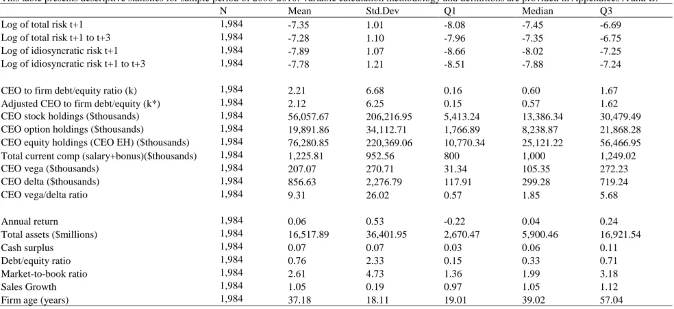
Panel A of Table 1 displays the summary statistics of k and k*, including key components of CEO compensation that are used as inputs to calculate k and k*. The
20
table also contains our dependent variables and additional regression control variables for fiscal years 2006-2010. Note that k and k* have high standard deviations and that there are some unusually high k and k* values in the sample. This finding is not surprising because, per Cassell et al. (2012), some firms have unusually small debt-to-equity ratios and rely less on debt-to-equity instruments to compensate their CEOs, resulting in higher CEO-specific debt-to-equity ratios.
[Insert Table 1]
In Figure 1, we show that the spread between k and k* widens as we move from Aaa down to Ccc. We also illustrate that the mean values of k and k* begin to increase after the 2008 credit crisis, which may indicate that inside debt holdings are becoming a more important component of CEO compensation.
[Insert Figure 1]
4.2. RESULTS FOR OLS ESTIMATION
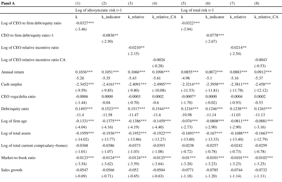
We replicate the main tests conducted by Cassell et al. (2012) where the independent variable is the original raw-k metric. We are careful to use similar methods, including the choice of documented control variables. In Table 2 we see results that are very similar to those of Cassell et al. (2012) for our sample from 2006-2010. Note that our sample period is longer than Cassell et al.’s, and this is likely the reason that our results vary slightly. In Panel A, we have the log of idiosyncratic risk (Columns 1-4) and the log of total risk for t+1 (Columns 5-8) as dependent variables, and in Panel B we
have the log of idiosyncratic risk (Columns 1-4) and log of total risk for t+3 (Columns 5-8) as dependent variables. The four explanatory variables21 are of largely negative significance in explaining the dependent variables, showing that CEOs with more inside debt implement more conservative corporate policies.
[Insert Table 2]
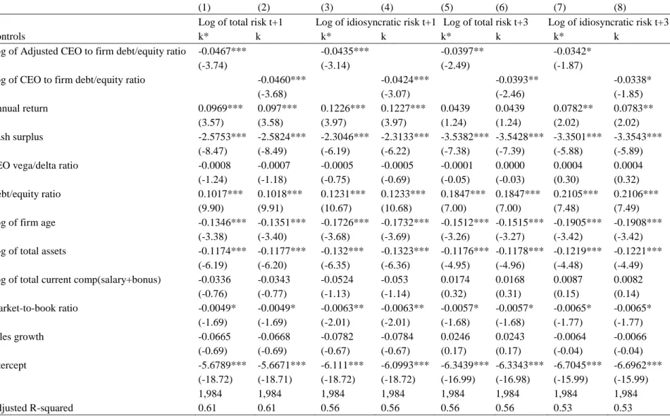
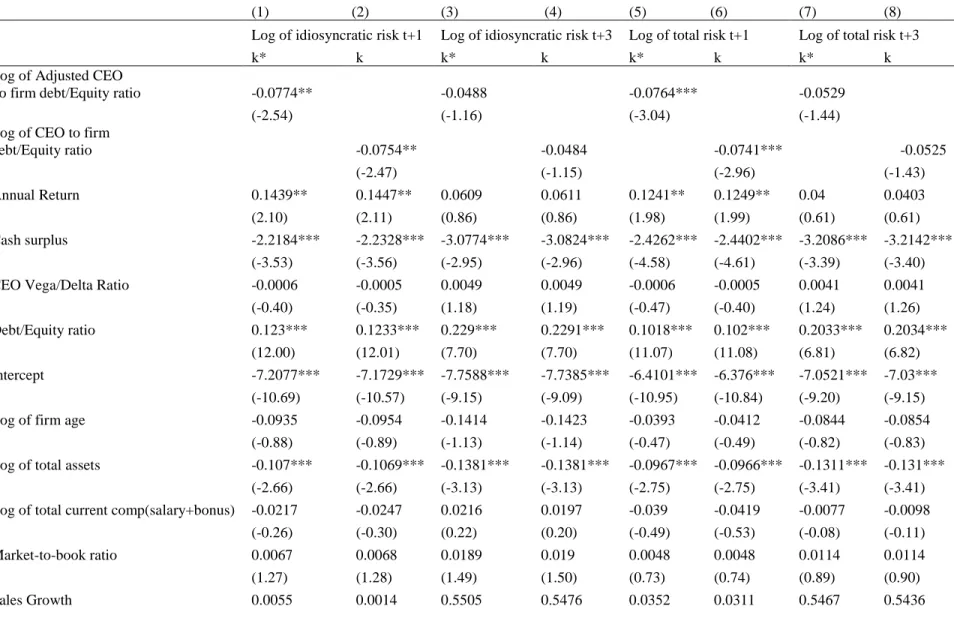
We next repeat the same analysis and instead use k* as the main explanatory variable. Recall that the calculation of k* requires several additional inputs, the overall effect of which is to reduce the sample size to 1,984 firm-year observations. In Table 3 we compare k and k* side by side, based on the same sample, and in each case the k* measure has a larger coefficient (in absolute value) and a larger t-stat than the original k.22 For example, in Columns (1-2) the coefficient on k* is -0.0467 with t-stat of -3.74, which are both larger than k’s coefficient of -0.0460 and its t-stat of -3.68. This pattern of k*’s superior ability to predict the dependent variables can be seen throughout Table 3.
[Insert Table 3]
While it appears at first glance that the improved fit offered by k* over k is nominal for the overall sample, the reader should keep in mind that the coefficient on k is already significant at the 1% critical level. In general, it is, empirically speaking,
2121 For detailed definitions of the four k measures, please refer to Cassell et al. (2011). For simplicity, we
use, throughout the paper, the k measure, the most used measure in Cassell et al. (2011). However the other three alternative measures generate similar results for all our tests.
22 For firms with little debt, the k or k* metrics can be artificially high, suggesting that the executive
22
difficult to improve upon an explanatory variable that is significant at such a high level. The fact that k* offers any improvement in fit is an empirical testament to its prowess. The obvious conceptual superiority of k* is, in general, supported empirically by the results in Table 3. Overall, the results presented in Table 3 support our main hypothesis,
H1.
4.3. A “HORSE RACE”
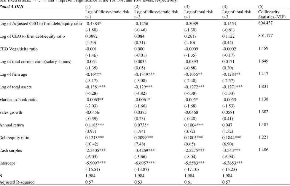
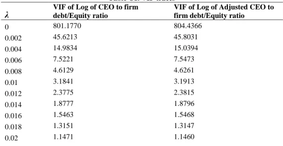
In order to directly compare the explanatory power of k and k*, we conduct a “horse race” by putting both measures in the same regressions. In Table 4 Panel A, the OLS results show that the coefficients of k become positive and insignificant, while the coefficients of k* remain negative, which is consistent with the theory, but insignificant. The extremely high VIF (Variance inflation factors) of k and k*, much higher than the rule-of-thumb value 10 (Belsley, 1991), indicates that the co-existence of k and k* leads to the multicollinearity problem, which increases the variance of the estimators and makes the estimated parameters unstable and insignificant (Kutner et al., 2004).
To address the multicollinearity problem, we follow Hoerl and Kennard (1970a, b) and Vinod (1978) by using ridge regression. Specifically, we estimate parameters via a “shrinkage” method that incorporates a small amount of bias into the estimating equation, thereby substantially reducing the sampling variance of the estimators in the presence of correlated data. See Appendix C for detailed discussion of ridge regression. The results in Table 4 Panel B show that k* outperforms k consistently, both in statistical
significance and economical significance. In particular, when included in the same regressions, k becomes insignificant while k* remains highly significant. Our risk-adjusted measure of inside debt seems, therefore, more relevant in determining firm risk.
[Insert Table 4]
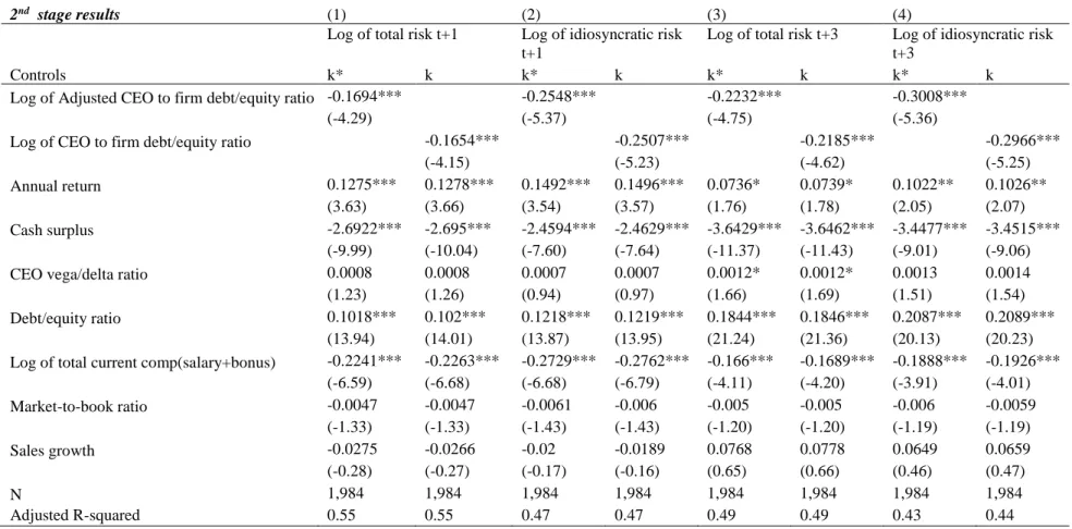
4.4. RESULTS FOR TWO-STAGE LEAST SQUARES ESTIMATION
We alternatively use two-stage tests designed to address endogeneity and utilize the same (except for one) choice of instrument variables as Cassell et al. (2012). We apply 2SLS in Table 5, repeating the same analysis as in Table 3. We use nearly identical instrumental variables (IV’s) as those used by Cassell et al. (2012), namely
CEO age, new CEO flag, natural logarithm of total assets and firm age, liquidity constraint flag, favorable tax status, maximum state tax rate on individual income, and
industry median inside debt measures. We only exclude CEO age as an IV because it is used in the computation of k*, thus creating a mechanical relation between CEO age and our adjusted inside debt measure. In our 2SLS analysis, we first regress k and k* on our instruments using equation (3), and then use the predicted values from the first-stage regression results as explanatory variables in equation (2).
In Columns 1-2 of Table 5, we see that k* has a coefficient of -0.1694 with a t-stat of -4.29, whereas k has a smaller coefficient of -0.1654 and a t-t-stat of -4.15 in explaining the log of total risk in year t+1. This pattern of k*’s superiority can be observed in Columns 3-4 as well. Consistent with the results presented in Table 3, the
24
conceptual superiority of k* is, in general, supported empirically by the results in Table 5. Overall, the results presented in Table 5 support our main hypothesis, H1.
[Insert Table 5]
4.5. RESULTS FOR INVESTMENT VS. NON-INVESTMENT GRADE FIRMS
As hypothesized earlier, we expect k* to exhibit a better fit for more credit risky firms where DP and RR discount the raw-k to greater degree. To investigate this aspect of our hypothesis, we examine k* for three subsamples: firms that are non-investment grade (this section); firms that experience credit downgrades (section 4.6); and firms with high credit risk (section 4.7). In all three cases we report results from OLS analysis. We also obtain similar qualitative results for 2SLS analysis.
By separating our sample into investment and non-investment grades, we find, as hypothesized, that k* performs better for the latter cohort. The difference for our sample split according to Moody’s credit ratings can be seen by contrasting the coefficients and t-stats in Columns 1-2 with those in Columns 3-4 of Table 6. Specifically, for the non-investment grade group (below Baa3), k* has a coefficient of -0.0477, larger (in absolute terms) than that of k at -0.0460. However, the coefficient for k* is not larger than the coefficient for k for the investment grade group (Baa3 or better). While the results reported in Table 6 are limited to the log of total risk at time t + 1, similar results are obtained for the other dependent variables. Overall, Table 6, when compared with Table
3, shows that the gap between the significance of k* and k widens both economically and statistically for non-investment grade firms.23 This is consistent with our hypothesis.
[Insert Table 6]
4.6. RESULTS FOR FIRMS EXPERIENCING CREDIT DOWNGRADES
We hypothesize that k* should outperform k even further for firms experiencing credit downgrades. To correctly identify these firms, we require firms to have at least two back-to-back annual credit rating observations. The subsample of firms with such observations is 1,092 (out of our 1,984 firms). Of these 1,092 firms, 410 experienced a credit rating downgrade (of one or more “notches”). Table 7 reports OLS analysis for these 410 cases. In general, the results reported are consistent with the notion that k* outperforms k for these firms, albeit results for the t+3 variables are statistically insignificant. Moreover, when comparing the coefficients on k* in Table 7 with those in Table 3, we see that the former are much larger (in absolute value), despite the smaller size of the downgrade subsample. Furthermore, when compared with Table 3, the improvement of k* over k appears more prominent, economically and statistically, in the results for t+1 (but not for t+3 since they are all insignificant). These results are generally consistent with H1 and further suggest that k* is a superior measure for credit risky firms.
23 We also investigated sample splits by above or equal to Ba3 versus below Ba3, and by above Caa1
versus equal to or below Caa1. Firms are classified as having “distressed debt” if their rating is Caa1 or worse. While the results of our investigation were generally consistent with the hypothesis that k*
26
[Insert Table 7]
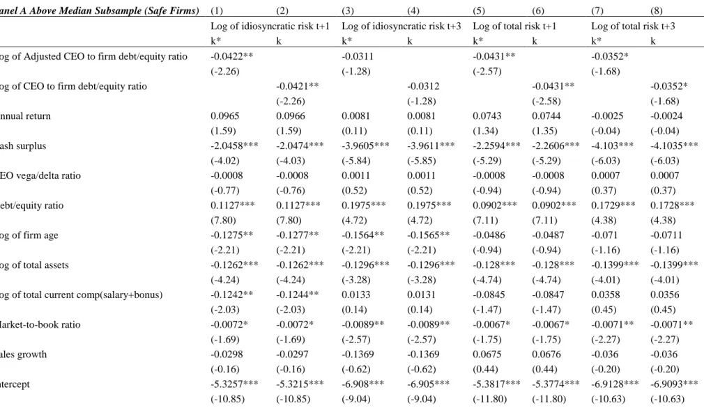
4.7. RESULTS FOR CREDIT RISKY FIRMS
As with non-investment grade firms and firms that experienced credit rating downgrades, we also expect k* to exhibit improved empirical fit for firms with higher-than-median [1-DP(1-RR)]. After all, [1-DP(1-RR)] is our unique “credit risk adjustment factor,” driving the difference between the promised payoffs and the expected payoffs of the inside debt. Table 8 Panel A suggests that for less risky firms, k and k* perform similarly. Note that if [1-DP(1-RR)]=1, k and k* are identical. In addition, if the firm is safe, the inside debt does not affect the managerial decision. Therefore, the results are less significant than those in Table 3.
We find interesting results in Panel B for credit risky firms. These are much more significant than those in Panel A and in Table 3, suggesting that inside debt does affect the executives’ decision in credit risky firms. More importantly, k* outperforms k even more in this subsample. This illustrates that the riskiness of inside debt is an important consideration, especially for credit risky firms.
[Insert Table 8]
5. Credit Crisis and Robustness Tests
In this section we conduct robustness checks to further test the relationship between k* and firm risk using OLS and 2SLS, and we discuss the results. We also
outline other robustness checks involving the derivation of DP and RR from credit default swap spreads.
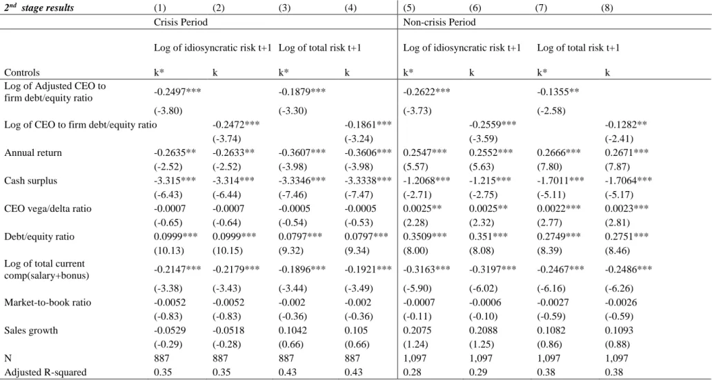
5.1. CREDIT CRISIS TEST
Assuming that the current credit crisis was an unanticipated exogenous shock to most individual firms, we use it as a natural experiment to address endogeneity (e.g., Campello, Graham, and Harvey, 2010; Ivashina and Scharfstein, 2010), and investigate whether the relation between executive conservatism (aggression) and credit risk-adjusted inside debt strengthens (wanes) during the crisis. We separate our sample into two sub-periods: the crisis period (2007 and 2008), and the non-crisis period (2006, 2009 and 2010). We then conduct 2SLS. The instruments used include new CEO flag, natural logarithm of total assets and firm age, liquidity constraint flag, favorable tax status, maximum state tax rate on individual income, and industry median inside debt measures. In Table 9, we first regress k and k* on our instruments, and then use the predicted values from the first-stage regression results as explanatory variables. Results are largely consistent with the inference that executives become more conservative during a credit crisis. For example, the t-statistics on the k* variables are generally greater during the crisis period, especially when the dependent variable is total risk. Also, results indicate that k* is still more robust than its original k as an explanatory variable throughout Table 9.
28
5.2. RESULTS OF ADDITIONAL ROBUSTNESS TESTS
As noted earlier, we also obtain DP and RR – for the full sample (1,984 firm- years) – by using alternative ratings data and their associated historical default probabilities and recovery rates provided by Standard and Poor’s. Furthermore, for a subsample of firms (318 firm years) we were able to impute DP and RR from 5-year credit default swap (CDS) spreads as provided by Bloomberg. Here we use firms whose inside debt maturity is close to five years. The method used to impute DP and RR from CDS spreads follows Hull (2012, pages 554-555).24 For the sake of brevity, we do not detail here the test results of relating future stock return volatility and k* as measured using these alternative values of DP and RR. Instead, we merely report that the robustness test results are highly consistent with those reported in all of the tables that are presented here. Results are available upon request. Given the efficiency of the credit markets and the rarity of split ratings, it is not surprising that results are similar when adjusting inside debt using data from different major ratings firms as well as CDS spreads. The values of the product [DP x (1 – RR)] obtained from different rating agencies, as well as from CDS spreads, are all highly correlated.25
24 DP can be readily implied from CDS spreads. To obtain RR, we rely on the empirical fact that implied
default probabilities are approximately proportional to 1/(1 – RR).
25 It is plausible that more credit risky firms are more conservative due to their debt restrictions/covenants,
rather than because of CEO choice/inside debt. However, tests involving raw-k already reflect restrictions associated with the firm’s outside debt. Since it is the same debt for both tests involving k* and k, the result that k* fits better than k suggests that executives must be more conservative, even if their outside debt precludes aggression. We show incremental explanatory power when using k*.
In unreported tests, we examined the other three k measures in Cassell et al. (2011): k_indicator, k_relative, k_relative_CA. We obtained similar comparative results by adjusting for the credit risk of the inside debt in each of the three cases. Different forms of k* perform consistently better than comparable forms of k, especially for firms with weaker credit.
We next investigate the possibility that a change in CEO may be driving our result that CEO aggression is inversely related to k*. For all tests reported in Tables 3-7, we separately investigate the 1,506 sample firms that experienced no change in CEO during the test period and find no difference in test results. For example, consistent with results reported in Table 6, k* outperforms k for non-investment grade firms within these 1,506 firms. This suggests that the possibility of differing degrees of managerial risk aversion, occasioned by CEO turnover, does not change our findings. Once again, our metric k* shows improvement over k in explaining future equity return volatility.
6. Conclusion
Jensen and Meckling’s (1976) theory of inside debt incentives predicts that more (less) credit risk-adjusted inside debt – and not merely the level of inside debt per se – motivates executives to be more (less) conservative. In this framework, our study makes three contributions to the literature on executive aggression and inside debt. First, to our knowledge, our study is the first one to provide a metric that reflects a credit risk-adjusted level of inside debt, and is therefore conceptually superior to previously used
30
metrics. Second, we show that the relation between our metric and future equity volatility is statistically and economically stronger than previously used metrics, especially for high-credit risk firms. In particular, we construct a metric, k*, that accounts for the credit risk-adjusted level of inside debt, and find that it is more powerfully related to corporate conservatism (as captured by future firm equity return volatility) than the commonly used raw-k metric. This relationship is more prominent for non-investment grade firms, firms experiencing a credit downgrade, and firms with high credit risk. As such, inferences from our study are important to researchers, practitioners, and policy makers when addressing the issue of optimal executive compensation, especially the use of inside debt. Third, we show that the relation between executive conservatism and inside debt heightens during the credit crisis.
Future research efforts should examine the relation between other corporate policies, such as accounting conservatism, tax aggression, diversification, research and development expenditures, and asset liquidity, and our k* metric, as well as the relation between corporate governance and the credit quality of inside debt.
References
Abhishek, S., S. Armitage, and J. Hagendorff. 2014. CEO inside debt holdings and risk-shifting: Evidence from bank payout policies. Journal of Banking and Finance 47, 41-53.
Allgood, S. and K.A. Farrell, 2000. The effect of CEO tenure on the relation between firm performance and turnover. The Journal of Financial Research 23, 373-390.
Anantharaman, D., V. Fang, and G. Gong. 2013. Inside debt and the design of corporate debt contracts. Management Science 60, 1260-1280.
Antia, M., Pantzalis, C., Park, J.C., 2010. CEO decision horizon and firm performance: an empirical investigation. Journal of Corporate Finance 16, 288–301.
Bebchuk, L.A., Jolls, C., 1999. Managerial value diversion and shareholder wealth.
Journal of Law, Economics, and Organization 15, 487–502.
Belsley, D. A., 1991. Conditioning diagnostics — Collinearity and weak data in regression. Wiley series in probability and mathematical statistics. New Jersey: Wiley-Interscience Publication.
Berle, A.A., Means, G.C., 1932. The Modern Corporation and Private Property, MacMillan, New York.
Black, F., Scholes, M., 1973. The pricing of options and corporate liabilities. Journal of Political Economy 81, 637–654.
Cassell, C., S. Huang, J. Sanchez, and M. Stuart. 2012. Seeking safety: The relation between CEO inside debt holdings and the riskiness of firm investment and financial policies. Journal of Financial Economics 103, 588-610.
Campello, M., Graham, J.R., Harvey, C.R., 2010. The real effects of financial constraints: evidence from a financial crisis. Journal of Financial Economics 97 (3), 470–487.
Chen, F., Dou, Y., Wang, X., 2010. Executive Inside Debt Holdings and Creditors’ Demand for Pricing and Non-pricing Protections, Working Paper, University of Toronto and Chinese University of Hong Kong.
Chen, D., Zheng, Y., 2014. CEO Tenure and Risk-taking. Global Business andFinance Review. 19(1), 1-27.
32
Chi, S., S. Huang, and J. Sanchez. 2014. CEO inside debt incentives and corporate tax policy. Working paper, University of Arkansas.
Choy, H., J. Lin, and M. Officer. 2014. Does freezing a defined benefit pension plan affect firm risk? Journal of Accounting and Economics 57, 1-21.
Coles, J., N. Naveen, and L. Naveen. 2006. Managerial incentives and risk-taking.
Journal of Financial Economics 79, 431-468.
Coles, J., Daniel, N., Naveen, L., 2013. Calculation of Compensation Incentives and Firm-related Wealth using Execucomp: Data, Program, and Explanation.
Core, J., Guay, W., 1999. The use of equity grants to manage optimal equity incentive levels. Journal of Accounting and Economics 28, 151–184.
Core, J., Guay, W., 2002. Estimating the value of employee stock option portfolios and their sensitivities to price and volatility. Journal of Accounting Research 40, 613–630. Daniel, N., Li, Y., and Naveen, L. 2013. No asymmetry in pay for luck. Working Paper. Edmans, A., and Q. Liu, 2011. Inside debt. Review of Finance 15, 75-102.
Eisdorfer, A., C. Giaccotto, and R. White. 2013. Capital structure, executive compensation, and investment efficiency. Journal of Banking and Finance 37, 549-562. Farebrother, R.W., 1975. The minimum mean square linear estimator and ridge regression. Technometrics, 127-128.
Farrell, K. A., D. A. Whidbee, 2002. Monitoring by the financial press and forced CEO turnover. Journal of Banking and Finance 26, 2249–2276.
Goyal, A., Santa-Clara, P., 2003. Idiosyncratic risk matters! Journal of Finance 58, 975– 1007.
Guay, W. 1999. The Sensitivity of CEO Wealth to Equity Risk: An Analysis of the Magnitude and Determinants. Journal of Financial Economics 53: 43-71.
Hoerl, A. E. and Kennard, R.W., 1970a. Ridge regression: biased estimation for nonorthogonal problems, Technometrics, 12, 55–67.
Hoerl, A. E. and Kennard, R. W., 1970b. Ridge regression: applications to nonorthogonal problems, Technometrics, 12, 69–82.
Hull, J. 2012. Options, Futures, and Other Derivatives, Prentice Hall, 8th edition.
Huson, M.R., P.H. Malatesta and R. Parrino, 2004. Managerial succession and firm performance. Journal of Financial Economics 74, 237-275.
Ivashina, V., Scharfstein, D., 2010. Bank lending during the financial crisis of 2008.
Journal of Financial Economics 97, 319–338.
Jensen, M. and W. Meckling. 1976. Theory of the firm: Managerial behavior, agency costs, and ownership structure. Journal of Financial Economics 3, 305-360.
Kabir, R., H. Li, and Y. Veld-Merkoulova. 2013. Executive compensation and the cost of debt. Journal of Banking and Finance 37, 2893-2907.
Kubick, T., G. Lockhart, and T. Robinson. 2014. Does inside debt moderate corporate tax avoidance? Working paper, University of Kansas.
Kutner, M. H., Nachtsheim, C. J., Neter, J., and Li, W., 2004. Applied linear statistical models (5th ed.). New York: McGraw-Hill.
Lambert, R.A., Larcker, D.F., 1987. An analysis of the use of accounting and market measures of performance in executive-compensation contracts. Journal of Accounting Research 25, 85–129.
Liu, Y., D. Mauer, and Y. Zhang. 2014. Firm cash holdings and CEO inside debt.
Journal ofBanking and Finance 42, 83-100.
Lowerre, J.M., 1974. On the mean square error of parameter estimates for some biased estimators. Technometrics, 461-464.
Merton, R.C., 1973. Theory of rational option pricing. The Bell Journal of Economics and Management Science 4, 141–183.
Moody’s, 2012. Corporate Default and Recovery Rates, 1920-2011. Moody’s Investors Service, 1–66.
Morck, R., Schleifer, A., Vishny, R.W., 1988. Management ownership and market valuation: an empirical analysis. Journal of Financial Economics 20, 293–315.
34
Murphy, K., 1985. Corporate performance and managerial remuneration: an empirical investigation. Journal of Accounting and Economics 7, 11–42.
Sundaram, R., and D. Yermack. 2007. Pay me later: Inside debt and its role in managerial compensation. Journal of Finance 62, 1551-1558.
Vinod, H.D., 1978. A survey of ridge regression and related techniques for improvements over ordinary least squares. Review of Economics and Statistics 60 (1), 121–131.
Wang, C., Xie, F., Xin, X., 2010. Managerial Ownership of Debt and Accounting Conservatism, Working Paper, Chinese University of Hong Kong and George Mason University.
Wei, C., and D. Yermack. 2011. Investor reactions to CEOs’ inside debt incentives,
Review of Financial Studies 24, 3813–3840.
Xu, Y., Malkiel, B.G., 2003. Investigating the behavior of idiosyncratic volatility.
Table 1 Summary statistics
This table presents descriptive statistics for sample period of 2006-2010. Variable calculation methodology and definitions are provided in Appendices A and B.
N Mean Std.Dev Q1 Median Q3
Log of total risk t+1 1,984 -7.35 1.01 -8.08 -7.45 -6.69
Log of total risk t+1 to t+3 1,984 -7.28 1.10 -7.96 -7.35 -6.75
Log of idiosyncratic risk t+1 1,984 -7.89 1.07 -8.66 -8.02 -7.25
Log of idiosyncratic risk t+1 to t+3 1,984 -7.78 1.21 -8.51 -7.88 -7.24
CEO to firm debt/equity ratio (k) 1,984 2.21 6.68 0.16 0.60 1.67
Adjusted CEO to firm debt/equity (k*) 1,984 2.12 6.25 0.15 0.57 1.62
CEO stock holdings ($thousands) 1,984 56,057.67 206,216.95 5,413.24 13,386.34 30,479.49
CEO option holdings ($thousands) 1,984 19,891.86 34,112.71 1,766.89 8,238.87 21,868.28
CEO equity holdings (CEO EH) ($thousands) 1,984 76,280.85 220,369.06 10,770.34 25,121.22 56,466.95 Total current comp (salary+bonus)($thousands) 1,984 1,225.81 952.56 800 1,000 1,249.02
CEO vega ($thousands) 1,984 207.07 270.71 31.34 105.35 272.23
CEO delta ($thousands) 1,984 856.63 2,276.79 117.91 299.28 719.24
CEO vega/delta ratio 1,984 9.31 26.02 0.57 1.85 5.68
Annual return 1,984 0.06 0.53 -0.22 0.04 0.24
Total assets ($millions) 1,984 16,517.89 36,401.95 2,670.47 5,900.46 16,921.54
Cash surplus 1,984 0.07 0.07 0.03 0.06 0.11
Debt/equity ratio 1,984 0.76 2.33 0.15 0.33 0.71
Market-to-book ratio 1,984 2.61 4.73 1.36 1.99 3.18
Sales Growth 1,984 1.05 0.19 0.97 1.05 1.12
Firm age (years) 1,984 37.18 18.11 19.01 39.02 57.04
36
Table 2 Association between the relative CEO debt-to equity ratio and the volatility of future stock returns
This table presents OLS regression results for our sample period of 2006-2010 in which the dependent variable is Log of total risk or Log of idiosyncratic risk. In Panel A, the dependent variable is measured in year t+1, and in Panel B, the dependent variable is measured in years t+1 through t+3. Variable calculation methodology and definitions are provided in Appendices A and B. For detailed definitions of the four k measures, please refer to Cassell et al. (2011). Each model includes industry (two-digit SIC) and year fixed effects. ***, **, and * represent significance at the 1%, 5%, and 10% levels, respectively.
Panel A (1) (2) (3) (4) (5) (6) (7) (8)
Log of idiosyncratic risk t+1 Log of total risk t+1
k k_indicator k_relative k_relative_CA k k_indicator k_relative k_relative_CA Log of CEO to firm debt/equity ratio -0.0327*** -0.0322***
(-3.46) (-3.94)
CEO to firm debt/equity ratio>1 -0.0836** -0.0778***
(-2.50) (-2.67)
Log of CEO relative incentive ratio -0.0210** -0.0214**
(-2.15) (-2.54)
Log of CEO relative incentive ratio CA -0.0026 -0.0043
(-0.28) (-0.53)
Annual return 0.1036*** 0.1051*** 0.1066*** 0.1096*** 0.0855*** 0.0872*** 0.0883*** 0.0912*** -5.26 -5.35 -5.43 -5.61 -4.98 -5.1 -5.16 -5.37 Cash surplus -2.3452*** -2.4161*** -2.4091*** -2.4905*** -2.3214*** -2.3958*** -2.3811*** -2.458***
(-9.59) (-9.85) (-9.80) (-10.08) (-11.53) (-11.81) (-11.78) (-12.12) CEO vega/delta ratio -0.0006 0.0000 -0.0003 0.0002 -0.0007* 0.0000 -0.0004 0.0002
(-1.44) -0.04 (-0.70) -0.6 (-1.70) (-0.02) (-0.93) -0.53 Debt/equity ratio 0.1493*** 0.1523*** 0.1517*** 0.1544*** 0.1216*** 0.1246*** 0.1238*** 0.1263***
-11.4 -11.58 -11.47 -11.6 -10.98 -11.14 -11.03 -11.13 Log of firm age -0.1331*** -0.1375*** -0.1386*** -0.1459*** -0.076*** -0.0808*** -0.0811*** -0.0881***
(-4.04) (-4.16) (-4.19) (-4.40) (-2.73) (-2.90) (-2.90) (-3.16) Log of total assets -0.1959*** -0.1936*** -0.1952*** -0.1922*** -0.1693*** -0.167*** -0.1688*** -0.1663***
(-14.02) (-13.77) (-13.86) (-13.27) (-13.60) (-13.33) (-13.40) (-12.79) Log of total current comp(salary+bonus) -0.0368 -0.0386 -0.0373 -0.0393 -0.0238 -0.0257 -0.0242 -0.0259 (-1.01) (-1.07) (-1.03) (-1.08) (-0.72) (-0.78) (-0.73) (-0.78) Market-to-book ratio -0.0123*** -0.0124*** -0.0124*** -0.0125*** -0.01*** -0.0101*** -0.0101*** -0.0102***
(-3.54) (-3.62) (-3.59) (-3.64) (-3.20) (-3.23) (-3.23) (-3.25) Sales growth -0.0547 -0.0566 -0.052 -0.0504 -0.0771 -0.0785 -0.0744 -0.0732
Intercept -5.6813*** -5.6149*** -5.6584*** -5.6339*** -5.3223*** -5.2582*** -5.3005*** -5.2728*** (-16.01) (-15.83) (-16.07) (-16.19) (-20.09) (-20.03) (-20.11) (-20.21)
N 3,899 3,899 3,899 3,899 3,899 3,899 3,899 3,899
Adjusted R-squared 0.58 0.57 0.57 0.57 0.62 0.61 0.61 0.61
Panel B (1) (2) (3) (4) (5) (6) (7) (8)
Log of idiosyncratic risk t+3 Log of total risk t+3
k k_indicator k_relative k_relative_CA k k_indicator k_relative k_relative_CA Log of CEO to firm debt/equity ratio -0.0327*** -0.0310***
(-2.77) (-3.10)
CEO to firm debt/equity ratio>1 -0.0987** -0.0856**
(-2.47) (-2.54)
Log of CEO relative incentive ratio -0.0204* -0.0199*
(-1.66) (-1.90) 0.0053 0.0016 (0.46) (0.16) Annual return 0.0714*** 0.072*** 0.0744*** 0.0782*** 0.0424** 0.0434** 0.0452** 0.0485** (2.74) (2.78) (2.87) (3.04) (1.99) (2.05) (2.13) (2.31) Cash surplus -3.0006*** -3.0559*** -3.0665*** -3.175*** -2.9305*** -2.991*** -2.9906*** -3.083*** (-8.47) (-8.60) (-8.61) (-8.85) (-10.24) (-10.34) (-10.41) (-10.63) CEO vega/delta ratio -0.0003 0.0003 0.0000 0.0006 -0.0004 0.0002 -0.0001 0.0005
(-0.49) (0.53) (0.05) (1.06) (-0.74) (0.45) (-0.16) (0.98) Debt/equity ratio 0.2141*** 0.2167*** 0.2166*** 0.22*** 0.1876*** 0.1902*** 0.1898*** 0.1928***
(9.33) (9.45) (9.41) (9.57) (8.90) (9.04) (8.99) (9.15) Log of firm age -0.1281*** -0.1308*** -0.1337*** -0.143*** -0.0831** -0.0865** -0.0882** -0.0962***
(-3.04) (-3.09) (-3.17) (-3.39) (-2.38) (-2.46) (-2.52) (-2.76) Log of total assets -0.1895*** -0.1877*** -0.1888*** -0.183*** -0.1745*** -0.1726*** -0.1739*** -0.1696***
(-10.05) (-9.98) (-9.94) (-9.47) (-10.85) (-10.75) (-10.72) (-10.23) Log of total current comp(salary+bonus) 0.0113 0.0097 0.0107 0.007 0.0209 0.0192 0.0204 0.0176
(0.22) (0.19) (0.21) (0.14) (0.48) (0.44) (0.47) (0.41) Market-to-book ratio -0.0175*** -0.0175*** -0.0176*** -0.0177*** -0.0148*** -0.0148*** -0.0149*** -0.015***
38 Sales growth -0.1197 -0.1227 -0.1168 -0.1137 -0.1156 -0.1179 -0.113 -0.1107 (-1.27) (-1.30) (-1.24) (-1.20) (-1.46) (-1.48) (-1.42) (-1.38) Intercept -6.3011*** -6.2306*** -6.2777*** -6.2664*** -5.9439*** -5.8793*** -5.9223*** -5.9054*** (-15.91) (-15.72) (-15.92) (-15.92) (-18.34) (-18.23) (-18.34) (-18.27) N 3,899 3,899 3,899 3,899 3,899 3,899 3,899 3,899 Adjusted R-squared 0.51 0.51 0.50 0.50 0.55 0.55 0.55 0.55