(Article begins on next page)
The Harvard community has made this article openly available.
Please share
how this access benefits you. Your story matters.
Citation
Lee, Charles M.C., Eric C. So, and Charles C.Y. Wang.
"Evaluating Firm-Level Expected-Return Proxies." Harvard
Business School Working Paper, No. 15-022, October 2014.
Accessed
February 17, 2015 4:52:59 AM EST
Citable Link
http://nrs.harvard.edu/urn-3:HUL.InstRepos:13350443
Terms of Use
This article was downloaded from Harvard University's DASH
repository, and is made available under the terms and conditions
applicable to Open Access Policy Articles, as set forth at
http://nrs.harvard.edu/urn-3:HUL.InstRepos:dash.current.terms-of-use#OAP
Copyright © 2014 by Charles M. C. Lee, Eric C. So, and Charles C.Y. Wang
Working papers are in draft form. This working paper is distributed for purposes of comment and discussion only. It may not be reproduced without permission of the copyright holder. Copies of working papers are available from the author.
Evaluating Firm-Level
Expected-Return Proxies
Charles M. C. Lee
Eric C. So
Charles C.Y. Wang
Working Paper
15-022
Expected-Return Proxies
Abstract
We develop and implement a rigorous analytical framework for empirically evalu-ating the relative performance of firm-level expected-return proxies (ERPs). We show that superior proxies should closely track true expected returns both cross-sectionally and over time (that is, the proxies should exhibit lower measurement-error variances). We then compare five classes of ERPs nominated in recent studies to demonstrate how researchers can easily implement our two-dimensional evaluative framework. Our empirical analyses document a tradeoff between time-series and cross-sectional ERP performance, indicating the optimal choice of proxy may vary across research settings. Our results illustrate how researchers can use our framework to critically evaluate and compare a growing body of ERPs.
I
Introduction
Expected rates of return play a central role in many managerial and investment decisions that affect the allocation of scarce resources. Recognition of this role has given rise to a substantial literature, spanning the fields of economics, finance, and accounting, about estimating expected rates of return for individual equities. The importance of firm-level estimates is widely understood, but consensus is lacking on how such estimates should be made. As a result, the specific estimation methods chosen by researchers vary widely across disciplines and studies, often without justification or discussion of alternative approaches.
Disagreement over how to estimate firm-level expected equity returns is exacerbated by the continued proliferation of new proxies proposed by researchers. One reason for this growth is the development of new asset-pricing models, each of which yields a spe-cific theoretical formulation of expected returns. For each such formulation, furthermore, researchers propose innovations to the inputs used when empirically implementing expected-returns proxies, such as new forecasting techniques for earnings or inclusion of additional asset-pricing factors.1 Thus, objectively comparing the relative merits of different firm-level
proxies requires a rigorous evaluative framework for adjudicating between them. This paper offers such a framework.
Our central contribution is a two-dimensional framework for empirically assessing the relative quality of firm-level expected-return proxies (ERPs). Using a firm’s true — but unobservable — expected-return as the normative benchmark, we define a given ERP’s de-viation from this benchmark as its measurement error. Although the measurement errors are themselves unobservable, we show that it is possible to derive characteristics of the dis-tribution of errors for each ERP, such that researchers can compare the relative performance of alternative proxies.
1For example, Gebhardt et al. (2001) use a residual-income model and analysts’ earnings forecasts to
estimate firms’ implied cost of equity capital. Subsequent researchers have modified this model by introducing the use of alternative growth forecasts (e.g.,Easton and Monahan,2005) and corrections for bias in analysts’ forecasts (e.g.,Easton and Sommers,2007), and/or by replacing analysts’ forecasts with mechanical earnings forecasts (e.g.,Hou et al.,2012).
Our two-dimensional framework evaluates ERPs on the basis of their relative time-series and cross-sectional measurement-error variances. Prior studies on the performance of ERPs have focused almost exclusively on cross-sectional tests, with mixed results (See Section II
for a discussion of this literature).2 We advance this literature by introducing the time-series dimension into the performance evaluation of firm-level ERPs.
Our framework formalizes the intuition that well-performing ERPs should both track expected returns in the cross-section (that is, cross-sectional variation in ERPs should re-flect cross-sectional variation in firms’ expected returns) and track a given firm’s expected returns closely over time (that is, time-series variation in a firm’s ERP should reflect varia-tion in its expected returns over time). Our framework allows researchers to characterize the cross-sectional and time-series dimensions of ERP performance for broad classes of firm-level proxies simultaneously and concisely. We show, both analytically and empirically, that the two dimensions of ERP performance are not redundant. We argue, further, that each can have a significant impact on research inferences in a given setting, and that researchers’ pref-erences over these dimensions should depend on the particular application and/or research context. Thus, the optimal measure produced by this framework will depend on each proxy’s cross-sectional and time-series performance and on the relative importance that a researcher assigns to each dimension.
To illustrate how researchers can implement our two-dimensional framework, we assess the relative performance of five families of ERPs (see Appendices I and II for a detailed description of each family). These five ERP families are based either on traditional equi-librium asset-pricing theory or on a variation of the implied-cost-of-capital (ICC) approach featured in accounting studies in recent years. Collectively, they encompass all of the proto-type classes of ERPs nominated by the academic literature in both finance and accounting over the past 50 years.
2Most prior tests judge ERPs based on their ability to predict subsequent realized returns. Standard
regression-based tests check whether the slope coefficient from a cross-sectional regression of ex-post returns on an ex-ante expected-returns proxy yields a coefficient of one (e.g.,Guay et al.,2011;Easton and Monahan,
Three of the ERPs we test originate in traditional equilibrium asset-pricing theory (the left-hand branch of the ERP tree depicted in AppendixI), in which non-diversifiable risk is priced, a firm’s ERP is a linear function of its sensitivity to each risk factor (the β’s), and the risk premium associated with the factor (the γ’s). We test a single-factor version based on the Capital Asset Pricing Model (CAPM) and a similar multi-factor version based on four empirically inspired factors (FFF). We also test a characteristic-based expected-return estimate (CER), discussed in Lewellen (2014), in which a firm’s factor loadings (the β’s) reflect its relative ranking in terms of each firm characteristic.
We also test two prototype ERPs from the ICC literature (the right-hand branch of the ERP tree in Appendix I). The implied-cost-of-capital is the internal rate of return that equates a firm’s market value to the present value of its expected future cash-flows; ICCs have become increasingly popular as a class of ERPs. We test a commonly used method of estimating ICC drawn fromGebhardt et al.(2001) andHou et al.(2012). Finally, we develop a new ERP prototype by computing a “fitted” version of theGebhardt et al.(2001) measure that we refer to as FICC. This proxy is new to the literature, but it seems to us to reflect a natural progression in the evolution of ERPs. FICC is based on an instrumental variable approach, whereby each firm’s ICC estimate is regressed on a vector of firm characteristics. Each firm’s FICC estimate is therefore a “fitted” value from the regression — that is, it is a linear function of the firm’s current characteristics.
Our results show that ICC, CER, and FICC dramatically outperform the traditional factor-based proxies (CAPM, FFF), both in the cross-section and in time-series. Among the three non-factor-based proxies, CER, the proxy nominated byLewellen(2014), performs best at exhibiting the lowest variance in cross-sectional measurement errors; the two implied-cost-of-capital proxies, ICC and FICC, perform better in the time-series tests. The performance of the new proxy, FICC, reflects its hybrid nature in that it offers lower cross-sectional measurement-error variance than ICC and relatively lower time-series measurement-error variance than CER. Our evidence is consistent with the findings of Lewellen (2014), which
show that characteristic-based proxies exhibit good return-predictability in the cross-section and suggest that these proxies may be more reliable than ICC proxies. However, we show that ICC proxies outperform CER in time-series. These findings suggest that, in research contexts where the cross-sectional variation of expected returns is of greater importance, such as in investments or capital budgeting, CER may be preferable. In contexts where time-series tracking of expected returns is of greater importance, such as studying the impact of certain shocks on firms’ expected returns (e.g., Callahan et al., 2012; Dai et al., 2013), ICC might perform best. When both time-series and cross-sectional performance are important, FICC might be the best option.
Overall, our empirical analyses give further credence to our two-dimensional framework by documenting a tradeoff between time-series and cross-sectional ERP performance, such that the optimal proxy may vary across research objectives and settings. We hope and expect that, by providing a rigorous tool for evaluating the relative performance of expected-return proxies, this framework will provide guidance on ERP selection and stimulate further thought and research on a matter of central import to researchers, investors, and corporate managers. The rest of the paper is organized as follows. Section II discusses related literature. Section III presents the theoretical underpinnings of our performance metrics. Section IV
provides details on our sample construction and empirical results. Section V concludes.
II
Related Literature
A large and growing literature examines the impact of regulation, managerial decisions, and market design on firm-level expected returns. For example, firm-level expected returns have been used variously to study the effect of disclosure levels (Botosan,1997;Botosan and Plumlee, 2005), information precision (Botosan et al., 2004), legal institutions and security laws (Hail and Leuz,2006;Daouk et al.,2006), cross-listings (Hail and Leuz,2009), corporate governance (Ashbaugh et al., 2004), accrual quality (Francis et al., 2004; Core et al.,2008), taxes and leverage (Dhaliwal et al., 2005), internal control deficiencies (Ashbaugh-Skaife
et al.,2009), voluntary disclosure (Francis et al.,2008), and accounting restatements (Hribar and Jenkins, 2004). In all of these studies, the research objective is to examine the effect of various elements in its information environment on a firm’s expected-return. Although these studies focus on factors affecting firm-level expected returns, they do not address the performance-evaluation problems that we identify here.
The specific methods of estimating expected returns chosen by researchers vary widely across studies and disciplines, often without justification or discussion of alternative ap-proaches.3 Furthermore, a related stream of research aims to develop new estimates of
expected returns, often by modifying existing proxies via the introduction of new inputs, such as forecasts of earnings or growth. The evaluation framework that we present here provides a means to compare the relative merits of existing proxies within a given research context; it also provides a tool to gauge whether a new proxy represents an advancement by using the performance of existing proxies as a minimum benchmark. By establishing how to implement this benchmark, our framework introduces clarity into a muddied and continually growing pool of potential ERPs.
The value of assessing ERPs within a two-dimensional framework is intuitive. In many decision contexts, such as investment and capital budgeting, we would like ERPs to reflect cross-sectional differences in true expected returns. In numerous other research contexts, however, it is crucial for time-series variation in a firm’s ERPs from one period to the next to reflect variations in the firm’s true expected returns — for example, when researchers use a difference-in-differences research design to study the impact of a regulatory change on a firm’s expected returns. In these settings the time-series dimension is more relevant, but existing performance tests do not assess the quality of ERPs along this dimension. Unlike prior studies that focus on cross-sectional differences in ERP performance (e.g., Easton and 3In recent years a substantial literature on ICCs has developed, first in accounting, and now increasingly
in finance. The collective evidence from these studies indicates that the ICC approach offers significant promise in dealing with a number of longstanding empirical asset-pricing conundrums. See Easton and Sommers(2007) for a summary of the accounting literature prior to 2007. In finance, the ICC methodology has been used to test the Intertemporal CAPM (Pástor et al.,2008), international asset-pricing models (Lee et al.,2009), and default risk (Chava and Purnanandam,2010).
Monahan, 2005), our time-series tests allow researchers to identify the most suitable ERP for tracking a firm’s expected-return variation over time in a particular context. Thus a key contribution of our paper is demonstrating how researchers can implement this critical second dimension of ERP performance evaluation.4
The paper most closely related to ours is Easton and Monahan (2005), hereafter re-ferred to as EM, which derives a methodology for relative comparisons of cross-sectional measurement-error variance between alternative ERPs. Our paper complements and ex-tends EM’s analysis in several ways. First, we argue and demonstrate that better-performing ERPs should track true expected returns not only in the cross-section but also over time, thus allowing researchers to more comprehensively assess the relative performance of ERPs. Second, EM’s framework is based on stricter assumptions, making it more difficult to ap-ply their methodology to compare broad classes of ERPs. Specifically, EM assumes that a proxy’s measurement errors are uncorrelated with true expected returns, making their measure inappropriate for a large class of ERPs. As a simple example, any ERP that is a multiple of true expected returns would violate the assumption necessary to use their ap-proach because the ERP’s error would be clearly correlated with the true expected-return. Third, our approach circumvents the requirement of the EM framework to estimate multiple firm-specific and cross-sectional parameters (e.g., cash-flow news); it is thus much simpler to implement empirically. Overall, though our cross-sectional measurement-error variance metric is conceptually similar to EM, our two-dimensional framework is more parsimonious, easier to implement, applicable to broad classes of ERPs, and it is more comprehensive by incorporating time-series performance evaluation.
In a related study, Botosan et al. (2011) proposes an alternative approach to evaluating ERPs, on the basis of their associations with risk proxies. A central difference between our 4We note that other papers have also examined time-series properties, in particular of ICCs. For example, Easton and Sommers (2007) examines the properties of aggregate risk premiums implied by ICCs and the role of analyst biases. Pástor et al.(2008) assess the time-series relations between aggregate risk prmiums and market volatility. Whereas these studies focus on the properties of aggregate expected returns, our framework focuses on the time-series performance of firm-level ERPs under a unified measurement-errors-based framework.
approach and that of Botosan et al. (2011) has to do with which construct is assumed to be valid. Botosan et al. (2011) assume that expected returns, as an economic construct, must entail certain associations with assumed risk proxies. Our approach relies on expected returns as a statistical construct, and our method relies on the properties of conditional expectations. Similarly, Larocque and Lyle (2013) proposes a framwork for assessing ERPs on the basis of their ability to predict accounting returns. The central difference between our approach and theirs is the assumed normative benchmark. Whereas our framework assumes the normative benchmark to be a firm’s true expected returns, their framework assumes the benchmark to be a firm’s future returns on equity.
III
Theoretical Underpinnings
This section begins with a simple decomposition of returns and then derives our two-dimensional evaluation framework for expected-return proxies.
Return Decomposition
We begin with a simple decomposition of realized returns:
ri,t+1 =eri,t+δi,t+1, (1)
where ri,t+1 is firm i’s realized return in period t+ 1, and δi,t+1 is the firm’s unanticipated news or forecast error.5 In this framework, we define er
i,t as the firm’s true but unobserved
expectation of future returns conditional on publicly available information at time t, cap-turing all ex-ante predictability (on the basis of the information set) in returns. By the property of conditional expectations, eri,t is optimal or efficient in the sense of minimizing
mean squared errors.6
5InCampbell(1991),Campbell and Shiller(1988a,b), andVuolteenaho(2002), the news term is further
decomposed into cash-flow and expected-returns components. This is not necessary for our purposes.
It follows from this definition and the property of conditional expectations that a firm’s expected returns (eri,t) cannot be systematically correlated with its forecast errors (δi,t+1), in time-series or in the cross-section.7 Intuitively, if expected returns were correlated with subsequent forecast errors, one could always improve on the expected-return measure by taking into account such systematic predictability, thereby violating the definition of an optimal forecast.8
Having thus defined our normative benchmark, we abstract away from the market-efficiency debate. If one subscribes to market market-efficiency, eri,t should only be a function
of risk factors and of expected risk premia associated with these factors. Conversely, in a behavioral framework,eri,tcan also be a function of other non-risk-related behavioral factors.
Next, we introduce the idea of ERPs (erbi,t+1), defined as the unobserved expected-return (eri,t+1) measured with error (ωi,t+1):
b
eri,t+1 =eri,t+1+ωi,t+1. (2)
In concept, eri,tb +1 need not be an ICC estimate as defined in the accounting literature — it can be any ex-ante expected-return measure, including a firm’s Beta, its book-to-market ratio, or its market capitalization at the beginning of the period. The key is that, whatever the “true” expected-return may be, we do not observe it. What we can observe are empirical proxies that contain measurement error. Our goal here is to evaluate how good a job these proxies do at capturing or tracking eri,t.
Differences between alternative ERPs are reflected in the properties (time-series and cross-sectional) of their ω terms. Comparisons between different ERPs are, therefore, com-parisons of the distributional properties of theω’s they generate, over time and across firms. Statements we make about the desirability of one ERP over another are, in essence, expres-sions of preference with regard to the properties of the alternative measurement errors (i.e.,
7Known as the Decomposition Property of conditional expectations (e.g.,Angrist and Pischke,2008). 8Fama and Gibbons (1982) make a similar argument in relating observed ex-post real interest rates to
the ω terms) that each is expected to generate. In other words, when we choose one ERP over another, we are specifying the loss function (in terms of measurement error) that we find least distasteful or problematic. The choice of ERPs thus becomes a choice between the attractiveness of alternative loss functions, expressed over ω space.
Under this setup, what would superior ERPs look like? We cannot nominate a single criterion by which all ERPs should be judged — doing so is impossible without specifying the researcher’s preference function over the properties of measurement errors. In our setup, however, “well-behaved” ERPs will exhibit certain empirical attributes. The extent to which they do so thus becomes a basis for comparison.
Comparing ERPs
Recall that our main objective is to produce ERPs that track true expected returns well, both across firms and over time. Equivalently, we would like measurement errors to be small at all times (i.e., ωi,t ∼0for alliand allt). Because these expectations are unlikely to hold,
we must choose between alternative error distributions, and specify those properties of ω
that are most important to us as researchers.
If the measurement errors (ω’s) are non-trivial, two further properties become important. First, we want measurement errors for a given firm that are stable over time. That is, all else equal, ERPs with lower time-series variance in measurement errors are preferred. If
ωi,t is stable over time, the ERP for a given firm will track its true expected returns more
closely in time-series. Consequently, changes in a firm’s ERP over time will be informative about changes in its underlying expected returns, rather than merely reflecting changes in ERP measurement errors. For example, an ERP with constant measurement errors over time is ideal, since its time-series variations will precisely reflect variations in the underlying unobserved expected returns. This is particularly useful in research contexts when studying the impact of regulation or disclosure policy on a firm’s expected returns (e.g., Callahan et al., 2012; Dai et al., 2013).
Second, we prefer measurement errors that are stable across firms at a given point in time. If this property holds, cross-sectional differences in ERPs are more informative about differences in expected returns between firms. For example, an ERP with constant mea-surement errors across firms is ideal, since differences in ERPs precisely capture differences in the underlying expected returns. This is particularly desirable in investment or capital budgeting decisions.
The stability of measurement errors over time and across firms is captured by the notion of lower measurement-error variance (in both time-series and cross-section). Thus, to capture how well ERPs track the underlying unobserved expected returns we propose two empirical properties by which to assess expected-return proxies: lower measurement-error variance in time-series and in the cross-section. Note that these two properties do not necessarily imply each other. As shown below, an ERP that exhibits perfect time-series tracking ability could exhibit noisy measurement errors in the cross-section; similarly, an ERP exhibiting perfect cross-sectional tracking ability could exhibit great intertemporal variations in measurement errors. This non-redundancy can also be seen in our empirical tests in Section IV.
Time-Series and Cross-Sectional Measurement-Error Variances
This section formalizes the two dimensions of ERP performance evaluation. The sub-sequent discussion presents the basic foundation and intuition of our evaluative framework. For brevity, most of the technical details appear in the Technical Appendix.
Time-Series Error Variance
To assess the stability of ERP measurement errors over time, we must be able to empir-ically identify and compare the time-series variance of the error terms, Vari(ωi,t), generated
by different ERPs. A key objective (and, we believe, contribution) of this paper is to ana-lytically disentangle the time-series properties of ERP measurement errors from those of the true expected returns, when both are time-varying and persistent over time.
We show in this sub-section (and in the Technical Appendix), that it is possible to derive an empirically estimable and firm-specific measure, Scaled Time-Series Variance, denoted as SVari(ωi,t), that allows us to compare alternative ERPs in terms of their time-series
measurement-error variance, even when the errors themselves are not observable. This anal-ysis then provides the foundation for our comparison of ERPs.
The Technical Appendixprovides a detailed derivation ofVari(ωi,t)andSVari(ωi,t).
Un-der the assumptions that (a) expected returns and measurement errors are jointly covariance-stationary, and (b) future news is unforecastable, we show in equation (T7) in the Technical Appendix that the time-series measurement-error variance of a given ERP for firm i can be expressed as:
Vari(ωi,t) = V ari(erbi,t)−2Covi(ri,t+1,erbi,t) +Vari(eri,t), (3)
whereVari(erbi,t)is the time-series variance of a given ERP for firm i, Vari(eri,t)is the
time-series variance of firmi’s expected returns, andCovi(ri,t+1,erbi,t)is the time-series covariance
between a given ERP and realized returns for firm i in period t+ 1.
The first term on the right-hand-side shows that the (time-series) variance of a given ERP’s measurement error is increasing in the variance of the ERP [Vari(erbi,t)]. This is
intu-itive: as the time-series variance of measurement errors of a given ERP for firm i increases, all else equal, so will the observed variance of the ERP.
The second term on the right-hand side shows that the variance of the error terms for a given ERP is decreasing in the covariance of the ERP and future returns [Covi(ri,t+1,erbi,t)].
This is also intuitive: to the extent the within-firm covariance between a given ERP and future realized returns is consistently positive over time, the variance of the errors will be smaller. In other words, to the extent a given expected-return proxy consistently predicts variation in future returns for the same firm, time-series variation in that proxy is more likely to reflect variation in the firm’s true expected returns than in measurement errors.
Finally, notice that the third term, Vari(eri,t), is the time-series variance of firm i’s
true (but unobserved) expected returns. For a given firm, this variable is constant across alternative ERPs and therefore does not play a role in relative performance comparisons. In other words, we need only the first two terms of (2) to determine which expected-return proxy exhibits lower time-series variance in measurement errors. Accordingly, we define the sum of the first two terms of (2) as the Scaled TS Variance:
SVari(ωi,t) = Vari(erbi,t)−2Covi(ri,t+1,erbi,t). (4)
In our empirical tests, we compute for each ERP and each firm the relative error variance measure using (4), and then assess the time-series performance of ERPs based on the average of SVari across the N firms in our sample:
AvgSVarTS = 1 N
X
i
SVari(ωi,t). (5)
For a given sample, ERPs that exhibit lower average time-series measurement-error variances [Vari(ωi,t)] also exhibit lower average scaled TS variance (AvgSVarTS). All else equal, ERPs
with lower time-series measurement-error variances for a given sample are deemed to be of higher quality because time-series variation in the expected-return proxy is more likely to reflect changes in firms’ expected returns than is time-series variation in measurement errors. Note that AvgSVarTS facilitates relative comparisons across ERPs. If we impose addi-tional structure (that is, if we make stricter assumption about the time-series behavior of expected returns), it is possible to obtain an empirically estimable absolute measure of the time-series measurement-error variance.9 Note too that our time-series framework allows researchers to pick the best ERP for a specific firm on the basis of SVari(ωi,t).
9This can be done, for example, by assuming that expected returns and ERP measurement errors
fol-low AR(1) processes (e.g., Wang, 2014). The empirical tests in this paper, however, do not require such assumptions.
Cross-Sectional Error Variance
Although low time-series measurement-error variance is desirable, this criterion alone is not sufficient to assess the quality of an ERP. When choosing between two ERPs that track true expected-return equally well in time-series, we will unambiguously prefer the one whose errors are more stable in the cross-section, since cross-sectional variations in such proxies are likely to reflect the cross-sectional variation in true expected returns.
Employing similar logic, we show inPart Bof the Technical Appendix that it is possible to derive an empirically estimable and proxy-specific measure, Average Scaled Cross-Sectional Variance (AvgSVarCS), that allows us to compare the cross-sectional measurement-error variance of alternative ERPs. We show that the cross-sectional measurement-error variance of a given ERP for a given cross-section t can be expressed as:
Vart(ωi,t) =Vart(erbi,t)−2[Vart(eri,t) +Covt(eri,t, ωi,t)] +Vart(eri,t), (6)
whereVart(erbi,t) is a given ERP’s cross-sectional variance at time t, Vart(eri,t) is the
cross-sectional variance in firms’ expected returns at time t, and Covt(ri,t+1,erbi,t) is the
cross-sectional covariance between firms’ ERPs at timetand their realized returns in periodt+ 1. Since the cross-sectional variance in firms’ expected returns — the last term — is invari-ant across different ERPs, relative comparisons of cross-sectional ERP measurement-error variance can be made by comparing the Scaled Cross-Sectional Variance:
SVart(ωi,t) = Vart(erbi,t)−2[Vart(eri,t) +Covt(eri,t, ωi,t)]. (7)
In particular, our empirical tests assess the cross-sectional performance of ERPs based on the average of SVart across the T cross-sections in our sample:
AvgSVarCS = 1 T
X
t
Part B of the Technical Appendix shows that AvgSVarCS can be estimated by
1 T
X
t
Vart(eri,t)b −2Covt(ri,t+1,eri,t),b (9)
following assumptions similar to those that characterize the time-series case above. Equa-tion (9) indicates that, all else equal, an ERP’s average cross-sectional measurement-error variance is increasing in the cross-sectional variance of the ERP. In other words, when ERPs are noisier, there is more measurement error. The second term suggests that, all else equal, an ERP’s average measurement-error variance is decreasing to the degree that ERPs predict future returns in the cross-section. In other words, when the cross-sectional variation of an ERP captures more of the cross-sectional variation in realized returns, variations in proxies are more likely to reflect the true variations in expected returns.
The Two-Dimensional Framework
The two dimensions of our evaluation framework are not redundant. An ERP that performs well in time-series may perform very poorly in the cross-section. For example, an ERP can have firm-specific measurement errors that are constant across time, resulting in zero time-series measurement-error variance, but these measurement errors can obscure the cross-sectional ordering of expected returns across firms. Consider two stocks, A and B, with constant true expected returns of 10 percent and 2 percent respectively. Suppose that a particular ERP model produces expected-returns proxies of 2 percent and 10 percent for stocks A and B respectively. Such an ERP produces zero time-series measurement-error variance for both stocks, since the measurement errors are constant across time for each firm, but such an ERP mis-orders the stocks’ expected returns in the cross-section and produces cross-sectional error variance.
Conversely, an ERP that performs well in the cross-section may perform poorly in time-series. For example, an ERP can have time-specific measurement errors that are constant
across firms but vary over time, resulting in zero cross-sectional measurement-error variance but potentially substantial time-series measurement-error variance. Suppose again that the true expected returns of stocks A and B are always 10 percent and 2 percent, respectively. Now consider an ERP model that produces expected-return proxies for A and B of 13 percent and 5 percent in certain years, and 10 percent and 2 percent in other years. Such an ERP always correctly orders expected returns in the cross-section and exhibits constant measurement errors for each firm in the cross-section (i.e., zero measurement-error variance in each cross-section), but will produce time-series error variance. In this case, time-series variation in the proxies does not reflect variations in true expected returns, but it reflects variations in measurement errors. In sum, an ERP that is equal to true expected returns is clearly a “perfect” ERP in our framework. More broadly, as shown above, a perfect ERP in our framework may have non-zero measurement error, so long as these errors are (a) constant across time for a given firm and (b) constant in the cross-section for all firms.
As noted earlier, EM also derive a methodology to rank ERPs on the basis of their cross-sectional measurement errors using a measure they call the modified noise variable. Like us, their measurement facilitates relative comparisons of cross-sectional measurement-error variance between alternative ERPs. However, their measure is based on stricter assumptions. Specifically, EM assume that ERP measurement errors are uncorrelated with true expected returns, which makes their measure inappropriate for a large class of ERPs. For example, any ERPs of the formC×eri,t for some constantC would violate the assumptions necessary
to use this “modified noise variable” to compare cross-sectional measurement error variance. Interestingly, EM also assume, to facilitate the use of their empirical metric, that on average the difference in the cross-sectional covariance of ERP measurement errors (ω) and news (δ) is “second-order” between any pair of ERPs; taken to the extreme, this assumption is equivalent to our assumption of zero cross-sectional correlation between news and expected returns (and therefore their proxies and measurement errors), on average. Overall, our cross-sectional performance metric is conceptually similar to EM. But we believe that ours is more
parsimonious, easier to implement empirically, and applicable to broad classes of ERPs, and that it extends the scope of analysis to include time-series performance evaluation.
In sum, we have provided a rationale for a two-dimensional evaluation framework that compares ERPs under a set of minimalistic assumptions. Researchers can use equations (5) and (9) to gauge the relative performance of ERPs to determine the optimal choice for a given research context. The following section applies this evaluation framework to assess the merits of five representative ERP measures nominated by prior literature.
IV
Empirical Implementation
A key strength of our two-dimensional evaluation framework is that it can be implemented in a small set of empirical analyses and is thus easily portable across research settings. To illustrate how researchers can empirically implement our framework, this section supplements our theoretical analyses by evaluating the relative performance of five families of monthly expected-return proxies. These five ERP groups are based either on traditional equilibrium asset-pricing theory or on some variation of the ICC approach featured in accounting studies in recent years. Collectively, they span all the prototype classes of ERPs nominated by the academic finance and accounting literatures over the past 50 years.
Three of the ERPs we test originate in traditional equilibrium asset-pricing theory, where non-diversifiable risk is priced. Specifically, we test a single-factor version based on the Capital Asset Pricing Model (CAPM) and similar multi-factor version based on Fama and
French (1993). We also test a characteristic-based ERP presented in Lewellen (2014) in
which a firm’s factor loadings (the β’s) embody its relative ranking in terms of each firm characteristic.
We also test two prototype ERPs from the ICC literature (the right-hand branch of the ERP tree in Appendix I). ICC is the internal rate of return that equates a firm’s market value to the present value of its expected future cash-flows. Finally, we develop a new ERP prototype by computing a “fitted” version of the Gebhardt et al. (2001) measure based on
an instrumental-variable approach, whereby each firm’s ICC estimate is therefore a “fitted” value from the regression — i.e., a linear function of the firm’s current characteristics. This section outlines our sample-selection process and the methodologies underlying our estimates of expected-return proxies.
Sample Selection
We obtain market-related data on all U.S.-listed firms (excluding ADRs) from the Center for Research in Security Prices (CRSP) and annual accounting data from Compustat for the period 1977-2011. For each firm-month, we estimate five expected-return proxies using data from the CRSP Monthly Stock file and, when applicable, firms’ most recent annual financial statements. To be included in our sample, each firm-month observation must include information on stock price, shares outstanding, book values, earnings, dividends, and industry identification (SIC) codes. We also require each firm-month observation to include valid, non-missing values for each of our five expected-return proxies, detailed below. Our final sample consists of 1,549,530 firm-month observations, corresponding to 12,022 unique firms.
Factor-Based Expected-Return Proxies
Our empirical tests include two estimates of expected returns to those derived from standard factor models: CAPM and a four-factor model based on Fama and French (1993) that adds a momentum factor (the UMD factor obtained from Ken French’s data library). At the end of each calendar montht, we estimate the expected one-month-ahead returns as
b Et[ri,t+1] =rft+1+ J X j=1 ˆ βiEbt[fj,t] (10)
for each factor model (with J = 1,4factors), where rft+1 is the risk-free rate in periodt+ 1,
ˆ
stock and factors’ returns over the 60 months prior to the forecast date), and fj,t are the
corresponding factors in period t. Expected monthly factor returns are estimated based on trailing average 60-month factor returns.
We denote the capital-asset pricing model and a four-factor Fama-French type model as CAPM and FFF respectively. We estimate CAPM for each firm at the end of each calendar month using historical factor sensitivities. Specifically, we first estimate each firm’s Beta to the market factor using the prior 60 months’ data (from t −1 to t−60). CAPM is then obtained by multiplying the estimated Beta by the most recent 12 months’ compounded annualized market-risk premium (provided by Fama and French) and adding the risk-free rate. Similarly, FFF represents a four-factor based ERP computed using the Mkt-Rf, HML, SMB, and UMD factors and 60-month rolling Beta estimates.
Implied-Cost-of-Capital (ICC)
We use the methodology in Gebhardt et al. (2001) to estimate a firm’s implied-cost-of-capital. ICC is a practical implementation of the residual income valuation model that employs a specific forecast methodology, forecast period, and terminal value assumption.10 Specifically, the time-t ICC expected-returns proxy for firmi is the berICCi,t that solves
Pi,t =Bi,t+ 11 X n=1 Et[NIi,t+n] Et[Bi,t+n−1] −erb ICC i,t 1 +erbICCi,t n Et Bi,t+n−1 + Et[NIi,t+12] Et[Bi,t+11] −erbICCi,t b
erICCi,t 1 +erbICCi,t
11Et Bi,t+11 , (11) where Et NIi,t+n
is the n-year-ahead forecast of earnings estimated using the approach in
Hou et al.(2012). We estimate the book value per share,Bi,t+n, using the clean surplus
rela-tion, and apply the most recent fiscal year’s dividend-payout ratio(k)to all future expected earnings to obtain forecasts of expected future dividends, i.e., Et[Dt+n+1] =Et[NIt+n+1]×k.
10Also known as the Edwards-Bell-Ohlson model, the residual income model simply re-expresses the
divi-dend discount model by assuming that book value forecasts satisfy the clean surplus relation,Et[Bi,t+n+1] =
Et[Bi,t+n] +Et[N Ii,t+n+1]−Et[Di,t+n+1], where Et[Bi,t+n], Et[NIi,t+n], andEt[Di,t+n], are the time t
We compute ICC as of the last trading day of each calendar month for all U.S. firms (excluding ADRs and those in the Miscellaneous category in the Fama-French 48-industry classification scheme), combining monthly prices and total-shares data from CRSP and an-nual financial-statements data from Compustat.
Characteristic-Based Expected-Return Proxies
Following Lewellen (2014), we calculate a characteristic-based ERP, which we denote as CER, by first estimating a firm’s factor loadings to three characteristics. This measure is based on an instrumental-variable approach, whereby each firm’s returns are regressed on a vector of firm characteristics in each cross-section (i.e., using Fama-MacBeth regressions); then the historical average of the estimated slope coefficients is applied to a given forecast period’s observed firm characteristics to obtain a proxy of expected future returns.
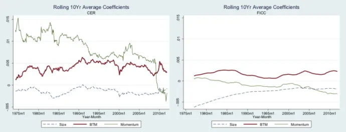
We also compute a “fitted” expected-return proxy, which uses ICCs instead of returns as the dependent variable. We refer to this fitted version of ICC, which represents a “fitted” value using historically estimated Fama-MacBeth coefficients, as FICC. We apply rolling 10-year Fama-MacBeth coefficients in our implementations of FICC and CER. Figure1reports rolling average Fama-MacBeth slope estimates from cross-sectional regressions of expected-returns proxies on firms’ size, book-to-market, and return momentum. The left-hand panel reports rolling average coefficients using realized returns as the dependent variable; the right-hand panel uses the ICC as the dependent variable. The coefficients from the ICC regressions are noticeably smoother than those from returns, consistent with FICC’s circumvention of some of the noise in returns by equating prices to estimates of future earnings.
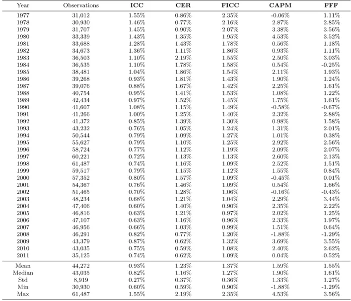
Descriptive Statistics
Table 1 reports the medians of five monthly expected-return proxies for each year from 1977 through 2011. We compute expected-return proxies for each firm-month in our main sample based on the stock price and on publicly available information as of the last trading
day of each month. Our sample consists of firm-months for which all five expected-return proxies are non-missing. The number of firm-months varies by year, ranging from a low of 30,930 in 1978 to a high of 61,487 in 1998. The average number of firm-months per year is 44,272, indicating that expected-return proxies are available for a broad cross-section of stocks in any given year. The time-series means of the monthly median expected-return proxies range from 0.93 percent (for ICC), to 1.59 percent (for CAPM).
It is instructive to compare the results for the two factor-based proxies (CAPM and FFF) with their non-factor-based counterparts (ICC, CER, and FICC). Recall that we compute CAPM and FFF using firm-specific Betas estimated over the previous 60 months and a continuously updated market-risk premium provided by Fama-French. The monthly means for CAPM and FFF (1.59 percent and 1.55 percent) are similar to those of the non-factor-based proxies. However, the time-series standard deviation of the factor-non-factor-based proxies is 3 to 5 times larger than the standard deviation of the non-factor-based proxies. Annual medians for CAPM range from -1.88 percent to 4.53 percent; in 5 out of 35 years the median of CAPM is negative, indicating that more than half of the monthly observations signal expected returns below zero. The volatility of CAPM and FFF reflects the instability of the market equity risk premium estimated on the basis of historical realized returns.
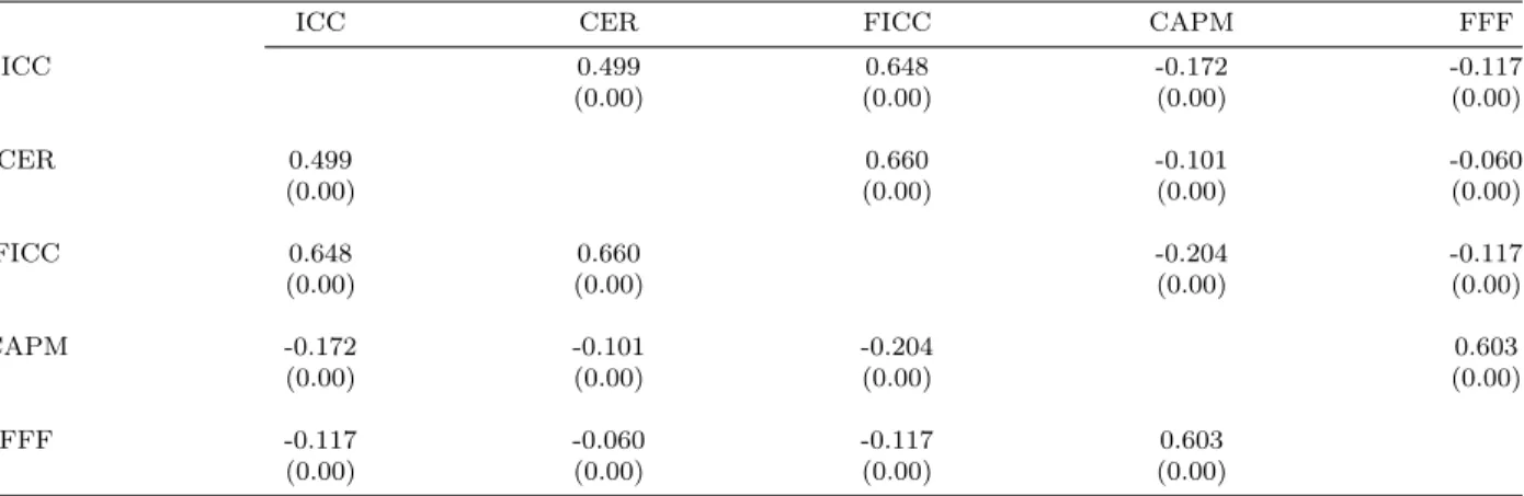
Table 2 reports the average monthly Spearman correlations among the five expected-return proxies. We calculate correlations by month and then average them over the sample period. The table shows that the three non-factor-based proxies are highly correlated among themselves, as are the two factor-based proxies. However, we find no positive correlation across the two groups — that is, none of the three non-factor-based proxies is positively correlated with the two factor-based proxies. In fact, the correlations between the non-factor-based and non-factor-based proxies are generally negative (finding consistent with earlier findings reported by Gebhardt et al.,2001).
Comparison of Measurement-Error Variances
As noted in Section III, better expected-return proxies should generate measurement errors with lower cross-sectional variance. Table3presents descriptive statistics for the cross-sectional variances of scaled measurement errors of the five expected-return proxies. Scaled measurement-error variances are calculated for each unique calendar-month/expected-return proxy pair using equation (7), as follows:
SVart(ωi,t) = Vart(erbi,t)−2Covt(ri,t+1,erbi,t),
where SVart(ωi,t) is the cross-sectional scaled measurement-error variance in month t, eri,tb
is the expected-return proxy in month t, and ri,t+1 is the realized return in montht+ 1.
Panel A of Table 3 reports summary statistics for the error variance from each model,
using a sample of data for 418 calendar months during our 1977-2011 sample period. Table values in this panel represent descriptive statistics for the error variance from each expected-return proxy computed across these 418 months.
Recall from Section III that we do not estimate the third component of Vart(ω) in
Equation (6); instead, we estimate the scaled measurement-error variances as in Equation (7). One implication of omitting this third term, which is a variance and therefore non-negative, is that the resulting estimates of scaled measurement-error variances can be negative. Hence, to ensure thatSVart(ωi,t)is positive, we multiply our estimates by 100 and add an arbitrary
constant of 10 when reporting summary statistics.
Panel Aof Table3shows that the three non-factor-based proxies (ICC, CER, and FICC)
generate smaller cross-sectional error variances than the other two. Panel B reports t-statistics based on Newey-West-adjusted standard errors corresponding to the pair-wise comparisons of cross-sectional scaled measurement-error variances within the sample of 418 months used in Panel A.
expected-return proxy displayed in the leftmost column has a larger (smaller) scaled measurement-error variance than the expected-return proxy displayed in the topmost row. The Panel B
findings indicate that all three non-factor-based proxies significantly outperform CAPM and FFF. Among the non-factor-based proxies, furthermore, both CER and FICC outperform the remaining three proxies, indicating that CER and FICC are best suited to rank firms in our sample in terms of their true expected returns.
According the second dimension of our evaluative framework, better expected-return proxies should also generate measurement errors with lower time-series variance. Table 4
reports a time-series measure of error variance for each of the five expected-return proxies, calculated for each unique firm/expected-return proxy pair using equation (4) as follows:
SVari(ωi,t) = Vari(erbi,t)−2Covi(ri,t+1,erbi,t),
where SVari(ωi,t) is the scaled measurement-error variance of firm i, erbi,t is the
expected-return proxy in montht, and ri,t+1 is the realized return in montht+ 1.
Panel A provides descriptive statistics for the variance of the error terms. To construct
this panel, we require each firm to have a minimum of 20 (not necessarily consecutive) months of data during our 1977-2011 sample period. A total of 12,022 unique firms met this data requirement. Table values in this panel represent summary statistics for the error variance (multiplied by 100) from each expected-return proxy computed across these 12,022 firms; again, we add a constant of 10 to each estimate before calculating summary statistics. Panel Breports t-statistics corresponding to the pair-wise comparison of firm-specific measurement errors across the sample of 12,022 firms used in Panel A.
The results in Table 4 show that the three non-factor-based proxies (ICC, CER, and FICC) generate lower time-series error variances than the other two. Panel B shows that ICC in particular generates measurement-error variances that are more stable over time than all other expected return proxies. Thus, the three non-factor-based proxies are not
merely better in the cross-section than the Beta-based proxies; they also behave better in time-series, on average.
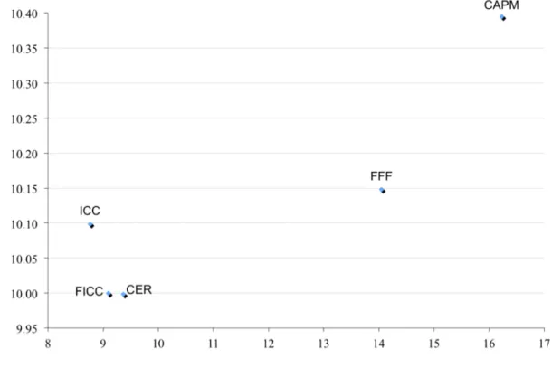
Figure 2 illustrates the results from our evaluative framework. The Y-axis depicts the median cross-sectional scaled measurement-error variance and the X-axis depicts the median time-series scaled measurement-error variances. Therefore, the upper left-hand corner of the figure demarcates an efficiency frontier where error variances are minimized.
This efficient frontier depicts the two-dimensional framework that researchers can use to compare alternative ERPs within their specific research setting. The figure shows that ICC, FICC, and CER are the best-performing proxies in terms of minimal error variance. The efficient frontier defined by these three proxies illustrates that the choice of expected-return proxies depends on the researcher’s particular loss function with respect to the stability of cross-sectional measurement errors versus the stability of time-series measurement errors. Strikingly, ICC, FICC, and CER all perform much better than the two factor-based measures, FFF and CAPM. The figure also illustrates the tendency for models that perform well on one dimension to do so on the other as well.
Why do certain proxies outperform others? Figure 2 helps to identify the relative strengths of the CER and ICC. CER performs better in terms of cross-section; ICC per-forms better in the time-series. One possible explanation for this phenomenon is that CER assumes a stable risk premium, relative to firm characteristics, based on a long panel of his-torical data (the estimated rolling coefficients on firm characteristics shown in AppendixII). These estimated risk premiums are relatively stable over time, while firm characteristics (i.e., risk factors) vary substantially. To the extent that risk premiums on these firm characteris-tics are moving over time, we would expect greater time-series measurement-error variances (though the cross-sectional ordering of expected returns may be less affected because firms are still sorted in each period according to their current risk factors).
Additionally, we find that ICC performs better in the time-series but not in the cross-section. To understand this result, recall that ICCs are fully forward-looking and do not rely
on estimating historical average premiums as CER does. Because estimating ICCs does not require calculating historical premiums, ICCs are more fluid across periods than CER; thus, ICC trades off decreased measurement errors in the time-series for increased measurement errors in the cross-section. These tradeoffs give further credence to our two-dimensional framework by empirically documenting a tradeoff between time-series and cross-sectional ERP performance, indicating that the appropriate proxy may vary across research objectives and settings.
Overall, our results offer a much more sanguine assessment of the implied-cost-of-capital approach than does some prior literature. A large and growing literature uses implied-cost-of-capital estimates as de-facto proxies for firm-level expected returns. However, prior research provides limited assurance that implied-cost-of-capital estimates are in fact useful proxies for expected returns. After examining seven implied-cost-of-capital estimates, for example, EM concluded that “for the entire cross-section of firms, these proxies are unreliable.” By contrast, we show that ERPs based on an implied-cost-of-capital approach (ICC, FICC) are attractive in terms of their cross-sectional performance, and also strongly outperform alternative ERPs in time-series tests.
Like those of Botosan et al. (2011), our findings raise questions about the EM assertion that ICC estimates are unreliable. Unlike Botosan et al. (2011), however, our primary evaluation criteria do not necessarily require superior ERPs to exhibit stronger empirical correlations with estimated Beta or other presumed risk proxies.
One caveat is that the conclusions drawn from our empirical analyses can depend on the sample used in the analysis (e.g.,Ecker et al.,2013) and on the variations of ERPs considered. The empirical exercise presented here is intended to illustrate the implementation of our two-dimensional evaluation framework for ERPs, but we hope that this framework will help researchers to determine which ERPs are appropriate for their intended research setting.
V
Conclusion
Estimates of expected returns play a central role in many managerial and investment decisions that affect the allocation of scarce resources in society. This study addresses a key problem in the literature that relies on estimates of expected returns: how to assess the relative performance of expected-returns proxies (ERPs) when prices are noisy.
Our paper demonstrates the importance of evaluating the time-series performance of ERPs, whereas most prior studies focus on cross-sectional performance evaluation. Evaluat-ing an ERP’s time-series performance is crucial in numerous research contexts, such as when researchers use a difference-in-differences research design to study the impact of a regulatory change on a firm’s expected returns.
We derive a two-dimensional evaluation framework that explicitly models both time-series and cross-sectional measurement-error variances for ERPs. Using a firm’s true but unobservable expected-return as the normative benchmark, we define an ERP’s deviation from this benchmark as its measurement error. Although the measurement errors themselves are unobservable, we show that it is possible to derive characteristics of the distribution of errors for each ERP such that researchers can compare the relative performance of alternative proxies.
Our main goal is less to establish the superiority of specific ERPs, than to demonstrate the value of an easily implementable performance-evaluation framework derived from a min-imalistic set of assumptions. We do not assume here that Beta or future realized returns are normative benchmarks by which ERPs should be measured. By establishing a rigorous evaluative framework, our findings help researchers select the appropriate ERP for a given context, and thus establish a minimum bar for what should be demanded from new entrants in the vast and still growing pool of firm-level expected-return proxies.
References
Angrist, J. D. and Pischke, J. 2008. Mostly harmless econometrics: An empiricist’s companion. Princeton University Press.
Ashbaugh, H., Collins, D., and LaFond, R. 2004. Corporate governance and the cost of equity capital. Working Paper, University of Wisconsin and University of Iowa.
Ashbaugh-Skaife, H., Collins, D., Kinney Jr., W., and Lafond, R. 2009. The effect of sox internal control deficiencies on firm risk and cost of equity. Journal of Accounting Research, 47(1):1–43.
Botosan, C. 1997. Disclosure level and the cost of equity capital. The Accounting Review, 72(3):323–349.
Botosan, C., Plumlee, M., and Wen, H. 2011. The relation between expected returns, realized returns, and firm risk characteristics. Contemporary Accounting Research, 28(4):1085– 1122.
Botosan, C., Plumlee, M., and Yuan, X. 2004. The role of information precision in deter-mining the cost of equity capital. Review of Accounting Studies, 9:233–259.
Botosan, C. A. and Plumlee, M. A. 2005. Assessing alternative proxies for the expected risk premium. The Accounting Review, 80(1):21–53.
Callahan, C. M., Smith, R. E., and Spencer, A. W. 2012. An examination of the cost of capital implications of fin 46. The Accounting Review, 87(4):1105–1134.
Campbell, J. 1991. A variance decomposition for stock returns. The Economic Journal, 101(405):157–179.
Campbell, J. and Shiller, R. 1988a. The dividend-price ratio and expectations of future dividends and discount factors. Review of financial studies, 1(3):195–228.
Campbell, J. and Shiller, R. 1988b. Stock prices, earnings, and expected dividends. Journal of Finance, 43(3):661–676.
Chattopadhyay, A., Lyle, M. R., and Wang, C. C. 2014. The cross section of expected returns around the world. Working Paper.
Chava, S. and Purnanandam, A. 2010. Is default risk negatively related to stock returns? Review of Financial Studies, 23(6):2523–2559.
Core, J. E., Guay, W. R., and Verdi, R. 2008. Is accruals quality a priced risk factor? Journal of Accounting and Economics, 46(1):2 – 22.
Dai, Z., Shackelford, D. A., Zhang, H. H., and Chen, C. 2013. Does financial constraint affect the relation between shareholder taxes and the cost of equity capital? The Accounting Review, 88(5):1603–1627.
Daouk, H., Lee, C., and Ng, D. 2006. Capital market governance: How do security laws affect market performance? Journal of Corporate Finance, 12(3):560–593.
Dhaliwal, D., Krull, L., Li, O., and Moser, W. 2005. Dividend taxes and implied cost of equity capital. Journal of Accounting Research, 43(5):675–708.
Easton, P. and Monahan, S. 2005. An evaluation of accounting-based measures of expected returns. The Accounting Review, 80:501–538.
Easton, P. and Sommers, G. 2007. Effect of analysts’ optimism on estimates of the expected rate of return implied by earnings forecasts. Journal of Accounting Research, 45(5):983– 1015.
Ecker, F., Francis, J., Olsson, P., and Schipper, K. 2013. Associations between realized returns and risk proxies using non-random samples. Working Paper.
Fama, E. and French, K. 1993. Common risk factors in the returns on stocks and bonds. Journal of Financial Economics, 33(1):3–56.
Fama, E. and French, K. 1996. Multifactor explanations of asset pricing anomalies. The Journal of Finance, 51:55–84.
Fama, E. and Gibbons, M. 1982. Inflation, real returns and capital investment. Journal of Monetary Economics, 9(3):297–323.
Francis, J., LaFond, R., Olsson, P. M., and Schipper, K. 2004. Costs of equity and earnings attributes. The Accounting Review, 79(4):967–1010.
Francis, J., Nanda, D., and Olsson, P. 2008. Voluntary disclosure, earnings quality, and cost of capital. Journal of Accounting Research, 46.1:53–99.
Gebhardt, W., Lee, C., and Swaminathan, B. 2001. Toward an implied cost of capital. Journal of Accounting Research, 39(1):135–176.
Guay, W., Kothari, S., and Shu, S. 2011. Properties of implied cost of capital using analysts’ forecasts. Australian Journal of Management, 36(2):125–149.
Hail, L. and Leuz, C. 2006. International differences in the cost of equity capital: Do legal institutions and securities regulation matter? Journal of Accounting Research, 44(3):485– 531.
Hail, L. and Leuz, C. 2009. Cost of capital effects and changes in growth expectations around u.s. cross-listings. Journal of Financial Economics, 93.3:428–454.
Hamilton, J. 1994. Time series analysis, volume 2. Cambridge University Press.
Hou, K., Van Dijk, M., and Zhang, Y. 2012. The implied cost of capital: A new approach. Journal of Accounting and Economics, 53:504–526.
Hribar, P. and Jenkins, N. 2004. The effect of accounting restatements on earnings revisions and the estimated cost of capital. Review of Accounting Studies, 9(2):337–356.
Larocque, S. and Lyle, M. R. 2013. Implied cost of equity capital estimates as predictors of accounting returns. Working Paper, Mendoza College of Business and Kellogg School of Management.
Lee, C., Ng, D., and Swaminathan, B. 2009. Testing international asset pricing models using implied costs of capital. Journal of Financial and Quantitative Analysis, 44(2):307–335. Lewellen, J. 2014. The cross section of expected stock returns. Critical Finance Review. Lintner, J. 1965. The valuation of risk assets and the selection of risky investments in stock
portfolios and capital budgets. The review of economics and statistics, pages 13–37. Pástor, L., Sinha, M., and Swaminathan, B. 2008. Estimating the intertemporal risk–return
tradeoff using the implied cost of capital. The Journal of Finance, 63(6):2859–2897. Sharpe, W. F. 1964. Capital asset prices: A theory of market equilibrium under conditions
of risk. The Journal of Finance, 19(3):425–442.
Vuolteenaho, T. 2002. What drives firm-level stock returns? Journal of Finance, 57(1):233– 264.
Wang, C. C. 2014. Measurement errors of expected return proxies and the implied cost of capital. Working Paper,Harvard Business School.
Technical Appendix
Part A. Ranking Firm-Specific ERP Measurement-Error Variance
Part A of this appendix derives a measure to rank ERP models on the basis of average time-series measurement-error variance, a measure that is ERP-specific and empirically es-timable. We call this measure Average Scaled TS Variance (AvgSVarTS). Our derivation proceeds in three steps. InStep 1we decompose a firm’s time-series ERP measurement-error variance and define a firm-specific Scaled TS Variance measure. In Step 2 we decompose realized returns and derive an expression for the time-series return-ERP covariance. InStep 3we show how to estimate Scaled TS Variance using the time-series return-ERP covariance and define the Average Scaled TS Variance.
We make the following assumptions throughout:
A1 Expected returns(eri,t+1), ERP measurement error(ωi,t+1), and realized returns(ri,t+1) are jointly covariance stationary.11
A2 Expected-returns forecast errors (or news, i.e., δi,t+1 = ri,t+1 −eri,t) is not ex-ante
forecastable, and is not systematically correlated with expected returns (in time-series or cross-section).
Step 1. Decomposing a Firm’s Time-Series Variance in ERP Measurement Errors and Defining M V arM V ari(ωi,t)M V arii(ω(ωi,ti,t))
We define an ERP as the sum of the true expected-return and its measurement error (T1):
b
eri,t+1 =eri,t+1+ωi,t+1. (T1) Taking the time-series variance on both sides of (T1) and re-organizing terms, a firm i’s time-series variance in ERP measurement errors can be written as
Vari(ωi,t) =Vari(erbi,t) +Vari(eri,t)−2Covi(eri,t,erbi,t), (T2)
which can be re-expressed as
Vari(ωi,t) =Vari(eri,t)b −2[Vari(eri,t) +Covi(eri,t, ωi,t)] +Vari(eri,t). (T3) The last right-hand-side term, firm i’s time-series variance in expected returns, does not depend on the choice of ERP model. Therefore, in comparing the time-series variance of ERP measurement errors for firm i, one needs only to compare the first two terms of (T3), which we refer to collectively as the Scaled Time-Series Variance of an ERP’s measurement
11A stochastic vector process {y
t}t≥1 is covariance-stationary if (a) E[yt] = µfor all t, and (b) E(yt−
µ)(yt−j−µ) =P
errors of firm i’s expected returns [SVari(ωi,t)]:12
SVari(ωi,t) =Vari(erbi,t)−2[Vari(eri,t) +Covi(eri,t, ωi,t)]. (T4)
Notice that the first right-hand-side term is firm i’s time-series variance in the ERP, which can be empirically observed. The second right-hand-side term involves unobservables: specifically, firm i’s variance in expected returns [Vari(eri,t)] and the time-series covariance between the firm’s expected returns and the ERP measurement errors [Covi(eri,t, ωi,t)]. In
what follows, we re-express the second term on the right-hand side in terms of variables that can be empirically observed.
Step 2. Decomposing Realized Returns and Time-Series Return-ERP Covariance In this step we show that Covi(ri,t+1,eri,t) =b Vari(eri,t) +Covi(eri,t, ωi,t). To obtain this
result, note that ex-post realized returns is the sum of the ex-ante expected returns and news or forecast errors:
ri,t+1 =eri,t+δi,t+1. (T5) We define eri,t to be firm i’s true but unobserved expected returns (eri,t) conditional on
publicly available information at timet, capturing all ex-ante predictability (with respect to the information set) in returns. By the property of conditional expectations, it follows that
eri,t is optimal or efficient in the sense of minimizing mean squared errors. This is known as
the Prediction Property of conditional expectations (e.g., Angrist and Pischke, 2008). It follows from this definition and the property of conditional expectations that a firm’s expected returns (eri,t) is uncorrelated with its forecast errors (δi,t+1) in time-series; this is also known as the Decomposition Property of conditional expectations (e.g., Angrist and
Pischke, 2008). Intuitively, if expected returns were correlated with subsequent forecast
errors, one could always improve on the expected-return measure by taking into account such systematic predictability, thereby violating the definition of an optimal forecast. This justifies assumption A2.
We can thus write the time-series covariance between returns and ERPs as:
Covi(ri,t+1,eri,t) =b Covi(eri,t+δi,t+1, eri,t +ωi,t)
=Vari(eri,t) +Covi(eri,t, ωi,t), (T6)
where the first equality follows from the return decomposition of (T5) and the definition of ERP (T1), and the last equality follows from assumption A2 (i.e., “news is news”), which implies that Covi(δi,t+1, eri,t) =Covi(ωi,t+1, δi,t+1) = 0.
Step 3. Estimating AvgSV arAvgSV arAvgSV arT ST ST S
Substituting (T6) into (T3) and (T4), we obtain:
Vari(ωi,t) =Vari(erbi,t)−2Covi(ri,t+1,erbi,t) +Vari(eri,t), (T7)
12Note thatVar
so that
SVari(ωi,t) = Vari(erbi,t)−2Covi(ri,t+1,erbi,t). (T8)
The first term of SVari shows that, all else equal, an ERP’s measurement-error variance is
increasing in the variance of the ERP. The second term of SVari shows that, all else equal,
an ERP’s measurement-error variance is decreasing in the degree to which ERPs predict future returns in time-series.
Notice that (T8) expresses SVari(ωi,t) in terms of two empirically observable variables
{erbi,t, ri,t+1}. These variables can be computed empirically, with consistency achieved under standard regularity conditions.13 Our empirical tests compute, for each ERP and each firm,
the relative error-variance measure using (T8), and assess the time-series performance of ERPs based on the average of SVari across the N firms in our sample:
AvgSVarTS = 1 N
X
i
SVari(ωi,t). (T9)
Notice also that SVari(ωi,t)≥ −Vari(eri,t), because Vari(ωi,t) =SVari(ωi,t) +Vari(eri,t)
and Vari(ωi,t) ≥ 0. Therefore, −Vari(eri,t) is the minimum bound for our empirically
estimable Scaled Time-Series Variance measure. In other words, if we have an ICC that measures expected returns perfectly, then SVari(ωi,t) =−Vari(eri,t).14
Part B. Ranking Cross-Sectional ICC Measurement-Error Variance
Here derive a measure to rank ERP models on the basis of their average cross-sectional measurement-error variance. We call this measure Average Scaled CS Variance (AvgSVarTS). Our derivation proceeds in two steps. In Step 1, we decompose a firm’s cross-sectional ERP measurement-error variance and define our cross-section-specific Scaled CS Variance measure. In Step 2, we show how to estimate Average Scaled CS Variance using the average cross-sectional return-ERP covariance. We make the same assumptions as inPart A.
13The following regularity conditions are sufficient to ensure that sample time-series variances and
covariances will converge in probability to population variances and covariances (Hamilton, 1994): for a covariance stationary stochastic process{Yt}t≥1, if there exists an MA(∞) representation (Yt=P∞j=0ψjj)
where the MA coefficients are absolutely summable (P∞
j=0|ψj| < ∞) and {t}t≥1 is an iid sequence with
E|t|r<∞, then the sample covariance converges to the population covariance in probability:
1 T PT t=1(Yt−Y¯T)(Yt−k−Y¯T)−→ p E(Yt−µ)(Yt−k−µ), where ¯ YT =T1P T t=1Ytandµ=E(Yt).
14Note that by comparing the resulting SVar for various ICC estimates, we only achieve a “relative”
performance assessment; we cannot conduct an “absolute” comparison to the true expected-returns measure without imposing further structure on the time-series process governing expected returns. InPart Cof this Technical Appendix, we illustrate how this can be done under the assumption that both the measurement error and the true expected returns follow AR(1) processes.
Step 1. Decomposing an ERP’s Cross-Sectional Measurement-Error Variance and Defining SVarSVarSVarttt(ω(ω(ωi,ti,ti,t)))
As in the case of time-series, the cross-sectional variance in ERP measurement errors can be written as
Vart(ωi,t) =Vart(erbi,t) +Vart(eri,t)−2Covt(eri,t,erbi,t), (C1)
which can be re-expressed as
Vart(ωi,t) =Vart(erbi,t)−2[Vart(eri,t) +Covt(eri,t, ωi,t)] +Vart(eri,t). (C2)
The final right-hand-side term, the cross-sectional variance in expected returns at time t, does not depend on the choice of ERP model. Therefore in comparing the cross-sectional variance of ERP measurement errors at timet, one needs only to compare the first two terms of (C2), which we refer to collectively as the Scaled CS Variance of an ERP’s measurement errors [SVart(ωi,t)]:15
SVart(ωi,t) = Vart(erbi,t)−2[Vart(eri,t) +Covt(eri,t, ωi,t)]. (C3)
Notice that the first right-hand-side term is the cross-sectional variance in the ERP, which can be empirically estimated. The second right-hand-side term involves unobservables — specifically, the cross-sectional variance in expected returns [Vart(eri,t)], and the
cross-sectional covariance between the firm’s expected returns and the ERP measurement errors [Covt(eri,t, ωi,t)].
Step 2. Defining and Estimating AvgSVarAvgSVarAvgSVarCSCSCS
In our empirical tests, we assess the cross-sectional performance of ERPs based on the average of SVart across the T cross-sections in our sample:
AvgSVarCS = 1 T
X
t
Vart(erbi,t)−2[Vart(eri,t) +Covt(eri,t, ωi,t)]. (C4)
To estimate AvgSVarTS, we note that the average cross-sectional covariance between returns and ERPs can be expressed as:
1 T X t Covt(ri,t+1,eri,t) =b 1 T X t
Covt(eri,t+δi,t+1, eri,t+ωi,t)
= 1 T
X
t
[Vart(eri,t) +Covt(eri,t, ωi,t)], (C5)
where the first equality follows from the realized returns decomposition (T5) and the defini-tion of expected-returns proxy (T1), and the last equality follows from the assumption (A2)
15Note thatVar