Predictive Inference with Copulas for Bivariate Data

(1)

Durham E-Theses

Predictive Inference with Copulas for Bivariate Data

MUHAMMAD, NORYANTI

How to cite:

MUHAMMAD, NORYANTI (2016) Predictive Inference with Copulas for Bivariate Data, Durham theses, Durham University. Available at Durham E-Theses Online: http://etheses.dur.ac.uk/11597/

Use policy

The full-text may be used and/or reproduced, and given to third parties in any format or medium, without prior permission or charge, for personal research or study, educational, or not-for-prot purposes provided that:

• a full bibliographic reference is made to the original source • alinkis made to the metadata record in Durham E-Theses

• the full-text is not changed in any way

The full-text must not be sold in any format or medium without the formal permission of the copyright holders. Please consult thefull Durham E-Theses policyfor further details.

Academic Support Oce, Durham University, University Oce, Old Elvet, Durham DH1 3HP e-mail: [email protected] Tel: +44 0191 334 6107

(2)

Predictive Inference with Copulas

for Bivariate Data

Noryanti Muhammad

A Thesis presented for the degree of

Doctor of Philosophy

Statistics and Probability Research Group

Department of Mathematical Sciences

University of Durham

England

(3)

My beloved husband; Imran, children; Aliah and Amirul, parents,

(4)

Predictive Inference with Copulas for Bivariate

Data

Noryanti Muhammad

Submitted for the degree of Doctor of Philosophy

February 2016

Abstract

Nonparametric predictive inference (NPI) is a statistical approach with strong fre-quentist properties, with inferences explicitly in terms of one or more future ob-servations. NPI is based on relatively few modelling assumptions, enabled by the use of lower and upper probabilities to quantify uncertainty. While NPI has been developed for a range of data types, and for a variety of applications, thus far it has not been developed for multivariate data. This thesis presents the first study in this direction. Restricting attention to bivariate data, a novel approach is presented which combines NPI for the marginals with copulas for representing the dependence between the two variables. It turns out that, by using a discretization of the copula, this combined method leads to relatively easy computations. The new method is introduced with use of an assumed parametric copula. The main idea is that NPI on the marginals provides a level of robustness which, for small to medium-sized data sets, allows some level of misspecification of the copula.

As parametric copulas have restrictions with regard to the kind of dependency they can model, we also consider the use of nonparametric copulas in combination with NPI for the marginals. As an example application of our new method, we consider accuracy of diagnostic tests with bivariate outcomes, where the weighted combination of both variables can lead to better diagnostic results than the use of either of the variables alone. The results of simulation studies are presented to provide initial insights into the performance of the new methods presented in this thesis, and examples using data from the literature are used to illustrate applications

(5)

of the methods. As this is the first research into developing NPI-based methods for multivariate data, there are many related research opportunities and challenges, which we briefly discuss.

(6)

Declaration

The work in this thesis is based on research carried out at the Statistics and Prob-ability Research Group, the Department of Mathematical Sciences, University of Durham, England. No part of this thesis has been submitted elsewhere for any other degree or qualification and it is all my own work unless referenced to the contrary in the text.

Copyright c 2016 by Noryanti Muhammad.

“The copyright of this thesis rests with the author. No quotations from it should be published without the author’s prior written consent and information derived from it should be acknowledged”.

(7)

Acknowledgements

Alhamdullilah, Allah my God, I am truly grateful for your countless blessings you have bestowed on me generally, and especially in accomplishing this thesis.

I would like to express my main deepest appreciation to my supervisors, Prof. Frank Coolen and Dr. Tahani Coolen-Maturi for their unlimited support, expert advice and guidance. Their patience, kindness, enthusiasm, and untiring support and calm advice have been invaluable to me.

I am immensely grateful to my husband, Muhamad Imran for his unwavering belief in me and unlimited support. His patience and kindness in helping to man-age the family, especially housework and our children, are really appreciated and respected. To my beloved children, Aliah and Amirul, thank you very much for understanding that your mom’s work kept her very busy.

Special thanks to my mother and mother-in-law for their frequent loving prayers for me, the substantial amount of their unconditional love surrounds me. To my great sadness, my father and father-in-law passed away on May 2014, they always encourage me to do the right things. To my brothers and sisters, thank you for your support and encouragement.

To all my friends who support and help me either directly or indirectly for this research, specifically by giving motivation and encouragement to finish this research, thank you so much. May God bless and ease whatever you do.

My final thanks to the Ministry of Higher Education of Malaysia (MOHE) and Universiti Malaysia PAHANG (UMP) for giving me the opportunity to pursue my studies at Durham University, supported by a full scholarship. Thanks also to the Department of Mathematical Sciences for offering such an enjoyable academic atmosphere and for the facilities that have enabled me to study smoothly.

(8)

Chapter 1 Introduction

1.1 Overview

Identifying and modelling dependencies between two or more related random quanti-ties is a main challenge in statistics and is important in many application areas. Tak-ing dependence into account is important to model, estimate and predict weather, risk and aspects of other applications more efficiently. Analyses of dependencies are of considerable importance in many sectors as an aid to better understanding the interaction of variables in a certain field of study and also as an input in every aspect of our life including engineering, health, finance, insurance and agriculture.

Statistical dependence is a relationship between any two or more characteristics of units under study or review. These units may, for example, be individuals, ob-jects, or various aspects of environment. The dependence structure is important in order to know whether a particular model or inference might be suitable for a given application or data set. Several types of dependence can occur, for example positive and negative dependence, exchangeable or flexible dependence and dependence de-creasing with lag (for data with a time index) [55]. A popular method for modelling dependencies is the use of a copula [14, 80]. Generally, a copula is a multivariate probability distribution for which the marginal probability distribution of each vari-able is uniform [55, 73]. Many researchers have addressed and studied dependence using copulas including Genest et al. [42], Embrechts et al. [36], Scaillet and Fer-manian [82] and Tsukahara [94]. Often, in their studies they estimate dependence

(11)

parameter(s). The dependence is also important in prediction where it plays a key role in decision making processes, classifying and other aspects that involve the de-pendence. For example, in risk of failure trajectory (e.g. effect of random external actions like wind, or unexpected reactions of the drivers), the dependence structure between vehicle criteria and safety acceptance of the models is considered to reduce road accidents rate [60].

This thesis presents a new method for predictive inference taking into account the dependence structure. It uses Nonparametric Predictive Inference (NPI) for the marginals combined with a copula. We restricted attention to bivariate data. The important general idea in this thesis is to look at the prediction of the two random quantities. We consider the dependence structure between these two ran-dom quantities using copula, as copula gives an interesting tool for describing the dependence structures. The idea that we considering the dependence structure be-tween the two random quantities using parametric copula for small data sets and nonparametric copula specifically kernel-based method for large data sets. The NPI on the marginals with the estimated copulas, presenting in this thesis is somewhat different to the usual statistical approaches based on imprecise probabilities [2]. Our method uses a discretized version of the copula which fits perfectly with the NPI method for the marginals and leads to relatively straight forward computations be-cause there is no need to estimate the marginals and the copula simultaneously. By using the NPI for the marginals, the information shortage is most likely to be about the dependence structure.

NPI has been developed over the last two decades, with many applications in statistics, reliability, risk and operations research (see www.npi-statistics.com). It has excellent frequentist properties, but relies on the natural ordering of the observed data or of a reasonable underlying latent variable representation with a natural ordering (e.g. used for Bernoulli and categorical observations [19]). So far, NPI has only been introduced for one-dimensional (univariate) data, this is the first thesis introducing a method which attempts to generalize NPI to bivariate data.

In Section 1.2 we present the main idea of NPI and a detailed outline of this thesis is given in Section 1.3, with details of related publications.

(12)

1.2. Nonparametric predictive inference 3

1.2 Nonparametric predictive inference

Nonparametric Predictive Inference (NPI) is a frequentist statistical framework for inference on a future observation based on past data observations [19]. NPI uses lower and upper probabilities, also known as imprecise probability [2], to quantify uncertainty and is based on only few assumptions.

NPI is based on the assumption A(n), proposed by Hill [50], which gives direct

conditional probabilities for a future real-valued random quantity, conditional on observed values of n related random quantities [1, 18]. Effectively, it assumes that the rank of the future observation among the observed values is equally likely to have each possible value 1, . . . , n+ 1. Hence, this assumption is that the next observation has probability 1/(n+ 1) to be in each interval of the partition of the real line as created by the n observations. Suppose that X1, X2, ..., Xn, Xn+1 are continuous

and exchangeable real-valued random quantities. Let the ordered observed values of

X1, X2, ..., Xnbe denoted byx(1) < x(2) < ... < x(n), letx(0) =−∞andx(n+1) =∞.

For a future observationXn+1, the assumption A(n) is

P(Xn+1 ∈(x(i−1), x(i))) =

1

n+ 1

for all i = 1,2, ..., n+ 1. We assume here, for ease of presentation, that there are no tied observations. These can be dealt with by assuming that such observations differ by a very small amount, a common method to break ties in statistics [51].

Inferences based onA(n)are predictive and nonparametric, and can be considered

suitable if there is hardly any knowledge about the random quantity of interest, other than then observations, or if one does not want to use any such further information in order to derive inferences that are strongly based on the data. The assumption

A(n) is not sufficient to derive precise probabilities for many events of interest, but

it provides bounds for probabilities via the ‘fundamental theorem of probability’ [30], which are lower and upper probabilities in imprecise probability theory [1, 2]. The lower and upper probabilities for event A are denoted by P(A) and P(A), respectively, and can be interpreted in several ways [18]. For example,P(A) (P(A)) can be interpreted as the supremum buying (infimum selling) price for the gamble on eventA, which pays 1 ifAoccur and 0 if not. Alternatively,P(A) (P(A)) can just be

(13)

regarded as the maximum lower (minimum upper) bound for a precise probability for A that follows from the assumptions made, we use this interpretation in this thesis. Generally, in imprecise probability theory [2], 0 ≤ P(A) ≤ P(A) ≤ 1 and

P(A) = 1−P(Ac_{) where} _Ac _{is the complement any event to} _A_{. These properties}

hold for all methods in this thesis.

NPI typically leads to lower and upper probabilities for events of interest, which are based on Hill’s assumption A(n) and have strong properties from frequentist

statistics perspective. As events of interest are explicitly about a future observa-tion, or a function of such an observaobserva-tion, NPI is indeed explicitly about prediction. The NPI lower and upper probabilities have a frequentist interpretation that could be regarded as ‘confidence statements’ related to repeated application of the same procedure. From this perspective, corresponding lower and upper probabilities can be interpreted as bounds for the confidence level for the event of interest. However, this method does provide neither predictions nor prediction intervals in the classical sense, as e.g. appear in frequentist regression methods. Prediction intervals tend to relate to confidence intervals for model parameter estimates combined with vari-ability included in the model, in NPI no varivari-ability is explicitly included in a model and there are clearly no parameters to be estimated.

Augustin and Coolen [1] proved that NPI has attractive inferential properties, it is also exactly calibrated from frequentist statistics perspective [62], which allows interpretation of the NPI lower and upper probabilities as bounds on the long-term ratio with which the event of interest occurs upon repeated application of statis-tical procedure. One attractive aspect of the NPI approach is that the amount of information available in the data is directly related to the differences between corresponding upper and lower probability, providing a new dimension to uncer-tainty quantification when compared to statistical methods which use only precise probabilities, such as standard Bayesian and frequentist methods including most commonly used nonparametric methods [23].

As mentioned in Section 1.1, NPI has been developed for a wide range of appli-cations as NPI methods are available for Bernoulli data [17], real-valued data [1], data including right-censored observations [24], ordinal data [34] and multinomial

(14)

1.3. Outline of the thesis 5 data [3, 20, 21].

1.3 Outline of the thesis

In Chapter 2 we introduce the main contribution of this thesis, novelty a new method for predictive inference which combines NPI for the marginals with an estimated parametric copula. We investigate the performance of this method via simulations, with particular attention to robustness with regard to the assumed copula in case of small data sets. A paper based on Chapter 2 has been accepted for publication in Journal of Statistical Theory and Practice [25]. In Chapter 3 we combine NPI with nonparametric copulas specifically using a kernel-based method, and we investigate the performance of this method via simulations. This chapter has been presented at the 23rd_{National Symposium on Mathematical Sciences (}_{Simposium Kebangsaan}

Sains Matematik Ke-23) at Malaysia and a short paper based on it was published in the conference proceedings [72]. We present and illustrate the application of the method proposed in Chapter 2 to a real world scenario in Chapter 4, concerning accuracy of diagnostic tests using Receiver Operating Characteristic (ROC) curves. In this chapter, we introduce a weighted average of bivariate diagnostic test results and we consider the dependence structure in order to maximise the accuracy of the tests involved on combined measurements. We study the performance of the method by simulations. This method raises interesting questions for future research, some brief comments and general conclusions are included in Chapter 5. In Chapters 2 - 4, illustrative examples are presented using data from the literature. In addition to the presentation of results for Chapter 3 mentioned above, this chapter have been regularly presented at several seminars and conferences, including at Northern Postgraduate Mini-Conference in Statistics (NPMCS) 2014, Newcastle University (Oral presentation), Royal Statistical Society (RSS) 2014 International Conference at Sheffield (Poster presentation), Durham Risk Day conference 2014 at Durham (Poster presentation), 4th Annual Survival Analysis for Junior Researchers Confer-ence 2015 at Keele University (Poster presentation), NPMCS 2015 at Durham Uni-versity (Oral presentation) and European Meeting of Statisticians (EMS) 2015 at

(15)

Vrije University, Amsterdam (Poster presentation). For Chapter 4, the results have been presented at Statistics seminar (Oral presentation) and recently at Stat4Grads seminar (Oral presentation) in Durham University.

(16)

Chapter 2 NPI with parametric copula

2.1 Introduction

In this chapter, we present main contribution of this thesis, a new novel method for predictive inference which combines NPI for the marginals with an estimated parametric copula. We propose a new semi-parametric method for predictive infer-ence for a future bivariate observation. The proposed method combines NPI in the marginals with an estimated copula to take dependence into account. The proposed method can be used with any parametric copula. Of course, if one has specific knowledge in favour of a particular family of copulas for the application considered, then using this family is most sensible and should lead to best results, if indeed this knowledge is correct. Any of the available methods to estimate the copula parame-ter can be used, where advantages and disadvantages of specific estimation methods are carried over. In our numerical studies, to investigate the performance of the proposed method and to illustrate its use, we will mention the specific estimation method applied.

Semi-parametric methods using copulas for statistical inference have been pre-sented before, see e.g. [13, 56, 94]. The main approach prepre-sented herein involves combining the empirical estimators for the marginals with a parametric copula, in nature this is close to the method presented in this chapter. Even more, Chen et al. [13] use a rescaled empirical estimator which, effectively, deals with the marginals in the same manner as the method used in this chapter. However, these presented

(17)

methods in the literature all consider estimation, while our approach in this thesis is explicitly developed for predictive inference.

In Section 2.2 we briefly give an introduction on copulas and specifically para-metric copulas. In Section 2.3 we introduce how NPI can be combined with an estimated parametric copula to provide a semi-parametric predictive method. Sec-tion 2.4 demonstrates how the proposed semi-parametric predictive method can be used for inference about different events of interest. In Section 2.5 we investigate the performance of this method via simulations, with particular attention to robustness with regard to the assumed copula in case of small data sets. Two examples are presented in Section 2.6 to illustrate application of the method to real world sce-narios, these examples use data from the literature. This method raises interesting questions for future research, some brief comments on this are included in Section 2.7.

2.2 Copula

Copula is a statistical concept for modelling dependence of random variables. The copula was invented and first used [73] by Sklar in 1959 [89]. Nelsen [73] presents a detailed introduction and overview. The word copula has been derived from the Latin word “copulare” which means to link, or to connect [36, 73], which is ap-propriate as the copula models the way in which random quantities are linked or connected.

By the well-known theorem by Sklar [89], every joint cumulative distribution function F of continuous random quantities (X, Y) can be written as F(x, y) =

C(FX(x), FY(y)), for all (x, y)∈R2, where FX and FY are the continuous marginal

distributions and C : [0,1]×[0,1]→[0,1] is a unique copula corresponding to this joint distribution. So, a copula is a joint cumulative distribution function whose marginals are uniformly distributed on [0,1] [14, 73].

Copulas have become popular tools for modelling dependence between random quantities in many application areas, including finance [14, 80], actuarial science [39, 79], risk management [36], hydrology [41] and reliability analysis [92]. Copulas

(18)

2.2. Copula 9 are attractive due to their ability to model dependence between random quantities separately from their marginal distributions [14, 73]. Throughout this thesis, atten-tion is restricted to bivariate data, the proposed methods can straightforwardly be generalized to more dimensional data but its performance would need to be stud-ied in detail, this is left as a topic for future research. In this thesis we use some parametric copula models and some nonparametric copula methods. Parametric copulas are used in this chapter and introduced below. Nonparametric copulas are introduced in Section 3.2.

Many parametric families of copulas have been presented in the literature, see e.g. [14, 55, 73]. In this research, we use four common bivariate one-parameter copulas, namely the Normal (or Gaussian), Clayton [15], Frank [38] and Gumbel [45] copulas, these are briefly reviewed below.

The Normal copula, with parameter θn, has cumulative distribution function

(cdf)

Cn(u, v|θn) = ΦB(Φ−1(u),Φ−1(v)|θn)

where Φ is the cdf of the standard normal distribution, and ΦB is the cdf of the

standard bivariate normal distribution with correlation parameterθn ∈(−1,1). The

Normal copula is easy to compute and to extend to more dimensions [66]. Moreover, the Normal copula is uniquely defined by the correlation of marginal distributions, thus it is easy to calibrate as this only requires calculating the pairwise correlation. However, Normal copula does not allow tail dependence to see modelled and it is symmetric, therefore it cannot capture interdependence among extreme events and does not allow asymmetric dependence among variables [66].

The Clayton copula [15] has cdf

Cc(u, v|θc) = max[(u−θc+v−θc −1)−1/θc,0]

with dependence parameter θc ∈ [−1,0)∪ (0,+∞). It is an asymmetric copula,

exhibiting greater dependence in the negative tail than in the positive. The Frank copula [38] has cdf

Cf(u, v|θf) = −θ_f−1ln 1 + (e −θfu−₁₎₍_e−θfv −₁₎ e−θf −₁

(19)

with dependence parameter θf ∈(−∞,0)∪(0,+∞). It is a symmetric copula.

The Gumbel copula [45] has cdf

Cg(u, v|θg) = exp(−[(−lnu)θg + (−lnv)θg]1/θg)

with dependence parameter θg ∈ [1,+∞). The Gumbel copula (also known as

Gumbel-Hougaard copula [73]) is an asymmetric copula. The Gumbel copula models strong right-tail dependence and relatively weak left-tail dependence [93].

These four commonly used copulas all have their own characteristics as men-tioned above. There is a one-to-one relationship between the dependence parame-ters of these four copulas and the concordance measure Kendall’s tau, τ, as given in Table 2.1 [14], note that the Gumbel copula cannot be used to model negative dependence, so it can only correspond to τ ≥ 0, and Frank copula does not allow

τ = 0.

Family Parameter range τ

Normal θn∈(−1,1) _π2 arcsinθn Clayton θc∈[−1,0)∪(0,+∞) θc/(θc+ 2) Frank θf ∈(−∞,0)∪(0,+∞) 1−4/θf[1−D1(θf)] Gumbel θg ∈[1,+∞) 1−1/θg Note:D1(θ) = Rθ

0(x/θ)/(ex−1)dxis the first Debye function [14].

Table 2.1: Relationship between dependence parameters and Kendall’s tau, τ

Many methods to estimate the parameter of a copula have been presented in the literature, see e.g. in [14, 80, 93]. There are several well known methods for estimat-ing the parameter of a parametric copula, such as maximum likelihood estimator (MLE), inference functions of margins (IFM) [55], pseudo maximum likelihood es-timation or canonical maximum likelihood [14] and method-of-moment [61]. The IFM estimation method is a two-stage estimation method which is based on MLE and is also known as multi-stage maximum likelihood (MSML) estimation [55]. This method allows us to estimate the parameters separately for the marginals and the copula. The method-of-moment approaches are based on the inversion of a consistent estimator of a moment of the copula, such as Spearmans rho, these are discussed

(20)

2.3. Combining NPI with a parametric copula 11 in detail in [61]. In the presentation of our method, we will denote a parameter estimate by ˆθ without the need to specify a particular estimation method.

There are advantages and disadvantages of the estimation methods, for example, MLE can be computationally intensive in the case of high dimensional distributions, because the number of parameters to be estimated simultaneously can be large. The problem might also occur when we have a very large sample size. The estimation of the estimator covariance matrices of the IFM is difficult both analytically and numerically due to the need to compute many derivatives in higher dimension [55], which should be considered when to generalize the method proposed to more than two dimensions. In addition, these two parametric methods are not robust against misspecification of the marginal distributions [58]. This problem has been argued by many researchers who advocate that the estimation of θ should not be affected by the choice of marginal distribution functions. The pseudo maximum likelihood estimation method solves this problem, it is discussed in details in Genest et al. [42] and in Shih and Louis [87].

2.3 Combining NPI with a parametric copula

In this section we present NPI with a parametric copula to provide a semi-parametric predictive method. The proposed semi-parametric predictive method consists of two steps. The first step is to use NPI for the marginals, the second step is to use a bivariate parametric copula and estimate the parameter value, to take the dependence structure in the data into account.

The first step is to use NPI for the marginals. Suppose that we have n bivariate real-valued observations (xi, yi), i = 1, . . . , n, which are the observed values of n

exchangeable bivariate random quantities. Henceforth, to simplify notation, we will actually use xi and yj to denote the ordered observations when considering the

marginals, so x1 < . . . < xi < . . . < xn and y1 < . . . < yj < . . . < yn. So it is

important that, with the plain indices now related to the separately ordered data related to the marginals, the valuesxiandyido not form an observed pair. It should

(21)

in the second step, where the parameter value of the assumed copula is estimated, the first step considers the marginals and hence only uses the information consisting of either the n observations xi or the n observations yj.

We are interested in prediction of one future bivariate observation, denoted by (Xn+1, Yn+1). Using the assumption A(n) we derive a partially specified predictive

probability distribution for Xn+1, given the observationsx1, . . . , xn, and similarly a

partially specified predictive probability distribution forYn+1, given the observations

y1, . . . , yn. These are as follows:

P(Xn+1 ∈(xi−1, xi)) =

1

n+ 1 and P(Yn+1 ∈(yj−1, yj)) = 1

n+ 1

for i, j = 1,2, . . . , n+ 1, where x0 =−∞, xn+1 =∞, y0 =−∞ and yn+1 = ∞ are

introduced for simplicity of notation.

To link this first step to the second step, where the dependence structure in the observed data is taken into account in order to provide a partially specified predictive distribution for the bivariate (Xn+1, Yn+1), we introduce a natural transformation of

these two random quantities individually. Let Xe_n₊₁ and Ye_n₊₁ denote transformed versions of the random quantities Xn+1 and Yn+1, respectively, following from the

natural transformations related to the marginalA(n) assumptions,

(Xn+1 ∈(xi−1, xi), Yn+1 ∈(yj−1, yj))⇐⇒ e Xn+1 ∈ i−1 n+ 1, i n+ 1 ,Yen+1 ∈ j−1 n+ 1, j n+ 1

fori, j = 1,2, . . . , n+ 1. This is a transformation from the real plane _R2 _{into [0}_,_1]2

where, based onn bivariate data, [0,1]2 is divided into (n+ 1)2 equal-sized squares. The A(n) assumptions for the marginals lead to

P(Xe_n₊₁ ∈ i−1 n+ 1, i n+ 1 ) = P(Xn+1 ∈(xi−1, xi)) = 1 n+ 1 P(Ye_n₊₁ ∈ j −1 n+ 1, j n+ 1 ) = P(Yn+1 ∈(yj−1, yj)) = 1 n+ 1

fori, j = 1,2, . . . , n+ 1. Note that, following these transformations of the marginals, we have discretized uniform marginal distributions on [0,1], which therefore fully correspond to copulas, as any copula will provide exactly the same discretized uni-form marginal distributions. Hence, this basic transuni-formation shows that the NPI

(22)

2.3. Combining NPI with a parametric copula 13 approach for the marginals can be easily combined with any copula model to reflect the dependence structure, leading naturally to the second step of our method.

The second step is to assume a bivariate parametric copula and estimate the parameter value. In this second step, the proposed method deals with the informa-tion, in the observed data, with regard to dependence of the two random quantities

Xn+1 and Yn+1. A bivariate parametric copula is assumed, with parameter θ. Using

the data, the parameter can be estimated by any statistical method, e.g. maximum likelihood estimation or a convenient (for computation) variation to it, resulting in a point estimate ˆθ. In order to correspond to the transformation method for the marginals, and to avoid having to consider the marginals whilst estimating the cop-ula parameter, at this stage we use also transformed data, where each observed pair (xi, yi),i= 1, . . . , n, is replaced by (rix/(n+ 1), r

y

i/(n+ 1)), withrix the rank of the

observation xi among the n x-observations (where the smallest value has rank 1),

and similarly ry_i the rank of yi among the n y-observations. It should be noticed

that, as this estimation process does not involve any estimation of the marginals, it can be performed in a computationally efficient manner, as it is often the simulta-neous estimation of the copula and related marginals that may cause computational difficulties in other statistical methods using copulas.

NPI on the marginals can now be combined with the estimated copula by defining the following probability for the event that the transformed pair (Xen+1,Yen+1) belongs

to a specific square from the (n+ 1)2 _{squares into which the space [0}_,_1]2 _{has been}

partitioned, hij(ˆθ) =PC(Xe_n₊₁ ∈ i−1 n+ 1, i n+ 1 ,Ye_n₊₁ ∈ j−1 n+ 1, j n+ 1 |θˆ) (2.1)

for i, j = 1,2, . . . , n + 1, with PC(·|θˆ) representing the copula-based probability

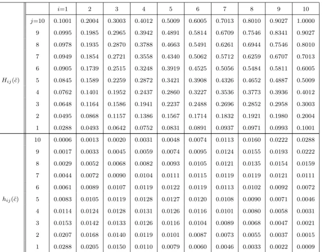
with estimated parameter value ˆθ, and the corresponding cumulative distribution function, Hij(ˆθ) =PC(Xen+1 ≤ i n+ 1,Yen+1 ≤ j n+ 1| ˆ θ) = i X k=1 j X l=1 hkl(ˆθ) (2.2)

Equations (2.1) and (2.2) can be represented by Figure 2.1. These (n+ 1)2 _values

(23)

Figure 2.1: Presentation of probabilities hij and Hij with an estimated copula

for the transformed future observations, which can be used for statistical inference on the actual future observation (Xn+1, Yn+1) or an event of interest involving this

bivariate random quantity, as explained in the next section. The probabilities hij

must satisfy the following conditions; 1. n X i=1 n X j=1 hij = 1 2. n X j=1 hij = 1 n+ 1,∀i∈(1, ..., n+ 1), and n X i=1 hij = 1 n+ 1,∀j ∈(1, ..., n+ 1) 3. hij ≥0,∀i, j = 1, ..., n+ 1.

These conditions will hold by the choice of a proper parametric copula. Note that, although a completely specified copula is used initially, for our inferences we only use the discretized version on the (n + 1)2 _{equal-sized squares with probabilities}

hij(ˆθ). In this discretized setting, hij(ˆθ) = ₍_n₊₁₎1 2 for all i, j = 1, . . . , n+ 1 would indicate complete independence of Xe_n₊₁ and Ye_n₊₁, and hence of X_n₊₁ and Y_n₊₁.

(24)

2.3. Combining NPI with a parametric copula 15 Furthermore, hij(ˆθ) = ₍_n₊₁₎1 for alli =j = 1, . . . , n+ 1 would correspond to

corre-lation 1 between these random quantities (both for the transformed and the actual future observations), while correlation−1 would correspond tohij(ˆθ) = ₍_n₊₁₎1 for all

j = (n+ 2)−i with i = 1, . . . , n+ 1. For example, consider n = 4 and the corre-sponding hij for −1.00 correlation, 1.00 correlation and no correlation are given in

Tables 2.2, 2.3 and 2.4. j = 5 0.2000 0.0000 0.0000 0.0000 0.0000 j = 4 0.0000 0.2000 0.0000 0.0000 0.0000 j = 3 0.0000 0.0000 0.2000 0.0000 0.0000 j = 2 0.0000 0.0000 0.0000 0.2000 0.0000 j = 1 0.0000 0.0000 0.0000 0.0000 0.2000 hij i= 1 i= 2 i= 3 i= 4 i= 5

Table 2.2: The probability of hij

j = 5 0.0000 0.0000 0.0000 0.0000 0.2000 j = 4 0.0000 0.0000 0.0000 0.2000 0.0000 j = 3 0.0000 0.0000 0.2000 0.0000 0.0000 j = 2 0.0000 0.2000 0.0000 0.0000 0.0000 j = 1 0.2000 0.0000 0.0000 0.0000 0.0000 hij i= 1 i= 2 i= 3 i= 4 i= 5

Table 2.3: The probability of hij

j = 5 0.0400 0.0400 0.0400 0.0400 0.0400 j = 4 0.0400 0.0400 0.0400 0.0400 0.0400 j = 3 0.0400 0.0400 0.0400 0.0400 0.0400 j = 2 0.0400 0.0400 0.0400 0.0400 0.0400 j = 1 0.0400 0.0400 0.0400 0.0400 0.0400 hij i= 1 i= 2 i= 3 i= 4 i= 5

(25)

2.4 Semi-parametric predictive inference

In this section, the semi-parametric predictive method presented in Section 2.3 is used for inference about an event which involves the next bivariate observation (Xn+1, Yn+1). LetE(Xn+1, Yn+1) denote the event of interest. LetP(E(Xn+1, Yn+1))

and P(E(Xn+1, Yn+1)) be the lower and upper probabilities, based on our

semi-parametric method, for this event to be true. As explained in the previous sec-tion, the observed data (xi, yi), i = 1, . . . , n, divide R2 into (n+ 1)2 blocks Bij =

(xi−1, xi)(yj−1, yj), for i, j = 1, . . . , n+ 1 (with, as before, x0 = −∞, xn+1 =

∞, y0 =−∞, yn+1 =∞ defined for ease of notation). Figure 2.2 shows the area of

blocks Bij = (xi−1, xi)(yj−1, yj), fori, j = 1, . . . , n+ 1.

Figure 2.2: Presentation of area of blocks Bij = (xi−1, xi)(yj−1, yj)

We further define

E(x, y) =  



1 if E(Xn+1, Yn+1) is true for Xn+1 =x and Yn+1 =y

(26)

2.4. Semi-parametric predictive inference 17 The fact that we work with a discretized probability distribution leads to imprecise probabilities as follows [2]. We defineEij = max

(x,y)∈Bij

E(x, y), soEij = 1 if there is at

least one (x, y) ∈ Bij for which E(x, y) = 1, else Eij = 0. Furthermore, we define

E_ij = min

(x,y)∈Bij

E(x, y), so E_ij = 1 if E(x, y) = 1 for all (x, y) ∈ Bij, else Eij = 0.

The semi-parametric method presented in the previous section leads to the following lower and upper probabilities for the event E(Xn+1, Yn+1),

P(E(Xn+1, Yn+1)) = X i,j E_ij hij(ˆθ) (2.3) P(E(Xn+1, Yn+1)) = X i,j Eij hij(ˆθ) (2.4)

Many events of interest can be considered with the summations over all i, j = 1, ..., n+ 1. Suppose, for example, that we are interested in the sum of the next observations Xn+1 and Yn+1, say Tn+1 = Xn+1+Yn+1. Then the lower probability

for the event that the sum of the next observations will exceed a particular value t

is

P(Tn+1 > t) =

X

(i,j)∈Lt

hij(ˆθ) (2.5)

with Lt = {(i, j) : xi−1 +yj−1 > t,1 ≤ i ≤ n + 1,1 ≤ j ≤ n + 1}, and the

corresponding upper probability is

P(Tn+1 > t) =

X

(i,j)∈Ut

hij(ˆθ) (2.6)

with Ut = {(i, j) : xi+yj > t,1≤ i ≤n+ 1,1≤ j ≤ n+ 1}. Equations (2.5) and

(2.6) represent the lower and upper survival functions for the future observation

Tn+1, based on our newly presented semi-parametric method, we denote these by

S(t) = P(Tn+1 > t) and S(t) = P(Tn+1 > t) and will use them in our analysis of

the predictive performance of our method in Section 2.5.

Before analysing the performance of this new semi-parametric method, it is useful to explain the idea behind it. As mentioned in Section 1.2, NPI has been developed over the last two decades for many applications and it has excellent frequentist prop-erties, but it relies on the natural ordering of the observed data (or on an assumed underlying latent variable representation with a natural ordering [19]). Moving to multivariate observations, however, causes problems due to the absence of a natural

(27)

ordering. At the same time, copulas have proved to be powerful tools to model de-pendence, and, as shown in Section 2.3, they can be linked in an attractive manner to NPI on the marginals, via discretization after a straightforward transformation. The resulting semi-parametric method is, however, a heuristic approach, in that it lacks the theoretical properties which make NPI for real-valued (one-dimensional) observations an attractive frequentist statistics method.

In Section 2.5 we show how the predictive performance of this method can be analysed, focussing on a case where interest is in the sum of Xn+1 and Yn+1. This

will also illustrate aspects of the imprecision in relation to the number of data observations and the dependence structure in the data.

2.5 Predictive performance

To investigate the predictive performance of the semi-parametric method presented in Sections 2.3 and 2.4, we conduct a simulation study. In each run of the simulation

N = 10,000 bivariate samples are generated, each of sizen+ 1, where we have used

n= 10,50,100. For each simulated sample, the firstn pairs are used as the data for the proposed semi-parametric predictive model, with the additional simulated pair used to test the predictive performance of this method.

In this analysis, we focus on the sum of of the next observations, so Tn+1 =

Xn+1+Yn+1, as presented in Section 2.4. Let (xji, y j

i) be the jth simulated sample,

consisting ofn pairs, so with subscripti= 1,2, . . . , n indicating the pair within one sample, and superscript j = 1,2, . . . , N indicating the specific simulated sample. Let (xj_f, yj_f) be the additional simulated (’future’) pair for sample j, and let the corresponding sum be denoted by tj_f =xj_f +y_fj, for j = 1,2, . . . , N. For q ∈(0,1), the inverse values of the lower and upper survival functions of Tn+1 in equations

(2.5) and (2.6), can be defined as

t_q =S−1(q) = inf t∈R {S(t)₆q} (2.7) tq =S −1 (q) = inf t∈R {S(t)₆q} (2.8)

(28)

semi-2.5. Predictive performance 19 parametric predictive method performs well if the two following inequalities hold,

p1 = 1 N N X j=1 1(tj_f _>tj_q)≤q (2.9) p2 = 1 N N X j=1 1(tj_f _>tj_q)≥q (2.10)

We will investigate the performance in this manner for q = 0.25,0.50,0.75. One could of course investigate different quantiles but these values will provide a good picture of the performance of the method, together with some particular aspects which are important to illustrate. To perform the simulation, we consider differ-ent values of Kendall’s τ in order to study the method under different levels of dependence. For each, we simulate from an assumed parametric copula with the parameter set at the value which corresponds toτ as presented in Table 2.1.

We consider two main scenarios. First, we actually assume in our semi-parametric method a copula from the same parametric family as used for simulation. Secondly, we use an assumed parametric copula in our method which differs from the copula used for the simulation. For the first case, we expect the method to perform well. Of course, this scenario is highly unlikely in practice, but it is important to study the performance of the method in this case, and the simulations will also enable study of the level of imprecision in the predictive inferences. The second scenario is more important, as it represents a more likely practical situation, namely where a parametric copula is assumed but this is actually not fully in line with the data generating mechanism. This can be considered as misspecification, and it is in such scenarios that we hope that our method will provide sufficient robustness to still provide relatively good quality predictive inference.

Given the simulated data in a single run, we estimate the parameter of the assumed parametric copula using the pseudo maximum likelihood method, which was briefly reviewed in Section 2.2 and is included in the R packageVineCopula[83]. We used this estimation method because we need to have a fast algorithm in order to use the copula parameter estimation as part of the method proposed in Sections 2.3 and 2.4. In addition, this method was considered the best estimation method

(29)

by [42]. However, any alternative estimation methods can be used; of course these may lead to slightly different results, but the overall performance of the method is unlikely to be affected much by minor differences in the estimation method. With the estimate ˆθ for the copula parameter, we obtain the probabilities hij(ˆθ) as given

in equation (2.1), and these form the basis for all possible inferences of interest. We have run N = 10,000 simulations with sample sizes n = 10,50,100, and with q= 0.25,0.50,0.75 andτ =−0.75,−0.5,−0.25,0,0.25,0.5,0.75. We restricted attention to the four parametric copulas discussed in Section 2.2, noting that the Frank copula does not allowτ = 0 and the Gumbel copula cannot be used to model negative dependence.

First, we applied our semi-parametric method with the assumed copula actually belonging to the same parametric family used for the data generation. Tables 2.5, 2.6, 2.7 and 2.8 present the results for the Clayton, Frank, Normal and Gumbel copula, respectively. These tables report the valuesp1 and p2 for the different values

of τ and n, as described in equations (2.9) and (2.10), for q = 0.25,0.50,0.75. For good performance of our method, we require p1 ≤ q ≤ p2. Furthermore, these

tables also present a value ˆθ, this is the average of the 10,000 estimates of the parameter, so for these tables this value is expected to be close to the value for θ

which corresponds directly to the τ used, and which is given in the second column of each table. However, we will not focus on these estimated values as it is really the predictive performance that is important to consider, due to the predictive nature of our approach. It is clear though that the parameter estimates tend to be closer to the real value for larger values ofn, which is of course fully as expected. It may be of interest to implement other estimation methods for the copula parameter, which may provide a slightly better performance, detailed study of this is left as a topic for future research.

Most cases in Tables 2.5, 2.6, 2.7 and 2.8 have q ∈ [p1, p2], which shows an

overall good performance of our semi-parametric predictive method, which is fully in line with expectations due to the use of the same parametric copula family in our method as the one that was actually used to simulate the data.

(30)

2.5. Predictive performance 21 First, for corresponding cases with increasing n, the imprecision, reflected through the difference p2 −p1, decreases. This is logical from the perspective that more

data allow more precise inferences, which is common in statistical methods using imprecise probabilities [2]. Indeed, if one increases the value ofnfurther, imprecision will decrease to 0 in the limit, where, informally, limit arguments are based on NPI for the marginals converging to the empirical marginal distributions, which in turn will converge to the underlying distributions, and with the assumed copula actually belonging to the same family as the one used to generate the data, this also will ensure an increasingly good performance of the method for increasingn.

A perhaps somewhat less expected feature of our method is seen by comparing corresponding cases with the same absolute value of τ, but negative τ compared to positiveτ. For such cases, the imprecisionp2−p1 is always greater with the negative

correlation than with the positive correlation, and this effect is stronger the larger the absolute value of the correlation. This feature occurs due to the fact that we are considering eventsTn+1 =Xn+1+Yn+1 > t, and can be explained by considering

the probabilitieshij(ˆθ) which are the key ingredients of our method for inference. In

case of positive correlation, thehij(ˆθ) tend to be largest for values ofiandj close to

each other, while for negative correlation this is the case for values of i and j with sum near to n+ 2, and this effect is stronger the larger the absolute value of the correlation. Calculating the lower and upper probabilities, equations (2.5) and (2.6) tends to include several more hij(ˆθ) values in the latter than in the former, and for

eventsTn+1 > tthese extrahij(ˆθ) included in the upper probability tend to have the

sum of their subscriptsiandj about constant. Hence, for positive correlation these extra hij(ˆθ) tend to include a few larger values for most values of t. For negative

correlation the effect is quite different, as then these extra hij(ˆθ) tend to include

relatively small values for small and for large values oft, in relation to the observed data, but when t is closer to the center of the empirical distribution of the values

xi+yi, corresponding to then data pairs (xi, yi), then many of the extra hij(ˆθ) are

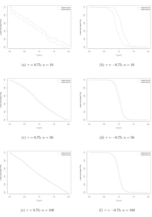
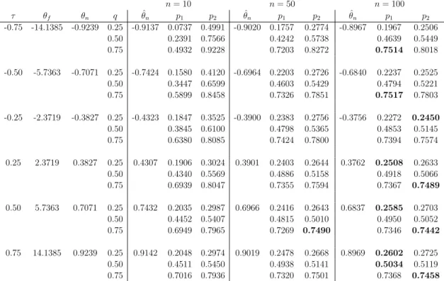
quite large, resulting in large imprecision. This effect can also be seen from plots of the lower and upper survival functions for Tn+1 shown in Figure 2.3 and Figure 2.4

(31)

n= 10 n= 50 n= 100 τ θ q θˆ p1 p2 θˆ p1 p2 θˆ p1 p2 -0.75 -6.0000 0.25 -9.7782 0.0806 0.5130 -5.8932 0.1859 0.2904 -5.8691 0.2233 0.2741 0.5 0.2171 0.7735 0.3963 0.5992 0.4428 0.5653 0.75 0.4770 0.9193 0.7009 0.7992 0.7376 0.7841 -0.5 -2.0000 0.25 -3.1214 0.1581 0.4114 -2.1369 0.2234 0.2732 -2.0693 0.2383 0.2653 0.5 0.3350 0.6711 0.4526 0.5545 0.4712 0.5286 0.75 0.5935 0.8427 0.7207 0.7710 0.7377 0.7640 -0.25 -0.6667 0.25 -1.3182 0.1995 0.3742 -0.7863 0.2436 0.2820 -0.7358 0.2405 0.2584 0.5 0.3919 0.6188 0.4743 0.5312 0.4840 0.5186 0.75 0.6381 0.8095 0.7235 0.7579 0.7354 0.7528 0.25 0.6667 0.25 1.3232 0.1737 0.2939 0.7934 0.2342 0.2587 0.7349 0.2380 0.2518 0.5 0.4289 0.5627 0.4784 0.5081 0.4876 0.5018 0.75 0.7143 0.8119 0.7451 0.7658 0.7457 0.7561 0.5 2.0000 0.25 3.0532 0.1836 0.2953 2.1431 0.2455 0.2711 2.0681 0.2380 0.2516 0.5 0.4487 0.5522 0.4962 0.5200 0.4916 0.5028 0.75 0.7091 0.7931 0.7460 0.7651 0.7479 0.7563 0.75 6.0000 0.25 10.1198 0.1970 0.2979 5.8992 0.2342 0.2596 5.8700 0.2458 0.2569 0.5 0.4587 0.5526 0.4922 0.5098 0.4933 0.5028 0.75 0.7132 0.8039 0.7337 0.7535 0.7427 0.7529

Table 2.5: Predictive performance, Clayton copula

survival functions forTn+1for the Normal and Gumbel copulas was very similar. For

all these copulas, positive correlation leads to imprecision for the events considered here being fairly similar over the whole range, while for negative correlation there is little imprecision in the tails but much imprecision near the center of the empirical distribution of the Tn+1.

(32)

2.5. Predictive performance 23 n= 10 n= 50 n= 100 τ θf q θˆf p1 p2 θˆf p1 p2 θˆf p1 p2 -0.75 -14.1385 0.25 -15.5793 0.0675 0.4846 -13.9428 0.1927 0.2960 -14.0058 0.2084 0.2677 0.50 0.2364 0.7453 0.4232 0.5663 0.4467 0.5270 0.75 0.4924 0.9249 0.6934 0.8006 0.7204 0.7784 -0.50 -5.7363 0.25 -6.9835 0.1578 0.4040 -5.8859 0.2263 0.2817 -5.7992 0.2320 0.2624 0.50 0.3494 0.6661 0.4635 0.5480 0.4725 0.5144 0.75 0.6092 0.8569 0.7282 0.7838 0.7259 0.7552 -0.25 -2.3719 0.25 -3.0634 0.1769 0.3533 -2.4751 0.2340 0.2727 -2.4138 0.2377 0.2572 0.50 0.3941 0.6099 0.4797 0.5323 0.4787 0.5088 0.75 0.6482 0.8207 0.7349 0.7688 0.7375 0.7580 0.25 2.3719 0.25 3.0129 0.2045 0.3026 2.4784 0.2364 0.2604 2.4088 0.2452 0.2549 0.50 0.4376 0.5583 0.4854 0.5135 0.4889 0.5048 0.75 0.6980 0.8052 0.7345 0.7583 0.7447 0.7580 0.50 5.7363 0.25 6.9335 0.1962 0.2989 5.8935 0.2382 0.2578 5.7972 0.2401 0.2526 0.50 0.4498 0.5517 0.4843 0.5075 0.4922 0.5025 0.75 0.7065 0.8052 0.7370 0.7568 0.7432 0.7554 0.75 14.1385 0.25 15.6739 0.1960 0.2898 13.8912 0.2429 0.2643 14.0050 0.2443 0.2551 0.50 0.4541 0.5487 0.4927 0.5127 0.4943 0.5053 0.75 0.7135 0.7998 0.7398 0.7607 0.7481 0.7557

Table 2.6: Predictive performance, Frank copula

n= 10 n= 50 n= 100 τ θn q θˆn p1 p2 θˆn p1 p2 θˆn p1 p2 -0.75 -0.9239 0.25 -0.9181 0.0854 0.5099 -0.9212 0.2002 0.3015 -0.9228 0.2202 0.2761 0.50 0.2477 0.7533 0.4187 0.5871 0.4566 0.5544 0.75 0.4911 0.9153 0.7045 0.8026 0.7311 0.7810 -0.50 -0.7071 0.25 -0.7462 0.1534 0.4002 -0.7235 0.2355 0.2919 -0.7169 0.2465 0.2691 0.50 0.3342 0.6466 0.4641 0.5529 0.4848 0.5292 0.75 0.5798 0.8355 0.7252 0.7797 0.7344 0.7604 -0.25 -0.3827 0.25 -0.4473 0.1942 0.3672 -0.4128 0.2406 0.2767 -0.3997 0.2408 0.2597 0.50 0.3943 0.6121 0.4728 0.5296 0.4894 0.5156 0.75 0.6386 0.8084 0.7303 0.7639 0.7412 0.7570 0.00 0 0.25 -0.0010 0.1877 0.3139 -0.0008 0.2362 0.2635 0.0000 0.2431 0.2566 0.50 0.4102 0.5723 0.4711 0.5105 0.4933 0.5141 0.75 0.6665 0.7971 0.7323 0.7626 0.7466 0.7598 0.25 0.3827 0.25 0.4478 0.1847 0.2956 0.4113 0.2279 0.2505 0.4004 0.2454 0.2556 0.50 0.4286 0.5538 0.4766 0.5074 0.4908 0.5026 0.75 0.6968 0.8057 0.7369 0.7580 0.7437 0.7540 0.50 0.7071 0.25 0.7469 0.2011 0.2931 0.7224 0.2394 0.2595 0.7164 0.2440 0.2525 0.50 0.4500 0.5554 0.4788 0.5033 0.4898 0.5026 0.75 0.7021 0.7978 0.7326 0.7537 0.7489 0.7602 0.75 0.9239 0.25 0.9174 0.2009 0.2865 0.9211 0.2430 0.2629 0.9224 0.2417 0.2524 0.50 0.4465 0.5441 0.4980 0.5168 0.4933 0.5039 0.75 0.6986 0.7961 0.7411 0.7607 0.7430 0.7527

(33)

n= 10 n= 30 n= 50 n= 100 τ θg q θfˆ p1 p2 θfˆ p1 p2 θfˆ p1 p2 θfˆ p1 p2 0 1.0000 0.25 1.2216 0.1735 0.2955 1.0699 0.2195 0.2642 1.0467 0.2311 0.2568 1.0266 0.2367 0.2515 0.5 0.4251 0.5871 0.4722 0.5331 0.4837 0.5199 0.4931 0.5113 0.75 0.7063 0.8231 0.7372 0.7827 0.7469 0.7753 0.7491 0.7636 0.25 1.3333 0.25 1.6911 0.1865 0.2861 1.4397 0.2237 0.2573 1.3973 0.2330 0.2548 1.3680 0.2451 0.2546 0.5 0.4288 0.5623 0.4695 0.5212 0.4776 0.5053 0.5008 0.5156 0.75 0.7032 0.8151 0.7355 0.7757 0.7396 0.7642 0.7551 0.7693 0.5 2.0000 0.25 2.6425 0.1961 0.2912 2.1723 0.2342 0.2684 2.1015 0.2371 0.2584 2.0514 0.2479 0.2582 0.5 0.4387 0.5488 0.4865 0.5257 0.4877 0.5128 0.5013 0.5134 0.75 0.7011 0.8072 0.7346 0.7710 0.7452 0.7673 0.7556 0.7679 0.75 4.0000 0.25 5.9120 0.2005 0.2870 4.1538 0.2335 0.2639 4.0598 0.2384 0.2575 4.0221 0.2502 0.2601 0.5 0.4557 0.5481 0.4835 0.5152 0.4881 0.5058 0.4997 0.5099 0.75 0.7012 0.7994 0.7287 0.7608 0.7384 0.7609 0.7445 0.7562

(34)

2.5. Predictive performance 25

(a) τ= 0.75;n= 10 (b)τ =−0.75;n= 10

(c) τ = 0.75;n= 50 (d)τ =−0.75;n= 50

(e) τ= 0.75;n= 100 (f) τ =−0.75;n= 100

(35)

(a) τ= 0.75;n= 10 (b)τ =−0.75;n= 10

(c) τ = 0.75;n= 50 (d)τ =−0.75;n= 50

(e) τ= 0.75;n= 100 (f) τ =−0.75;n= 100

(36)

2.5. Predictive performance 27 As mentioned before, the main idea of the new method presented in this chapter is to provide a quite straightforward method for prediction of a bivariate random quantity, where imprecision in the marginals provides robustness with regard to the assumed copula. This is attractive in practice, because one often has less knowledge about the dependence structure than about the marginals, in particular if one has a relatively small data set available. The practical usefulness of the method is therefore dependent on its ability to provide reasonable quality predictive inference in case one does not assume to know the parametric family of copulas, which generated the data, exactly. To study the performance of our semi-parametric predictive inference method, we perform simulations as before, but now we generate the data from one of the four mentioned copula families, while we assume a different parametric copula for the second step of our method. The simulations are further performed in the same manner as those above, with attention again on prediction of Tn+1 =Xn+1+Yn+1.

We report again first simulation results for just a few scenarios, the other com-binations of real and assumed copulas, out of the four parametric copula families discussed before, provided very similar results, as did repeated simulations of the same scenarios. Table 2.9 presents the results with data generated from the Frank copula whilst assuming the Normal copula in our method. While we mostly focus on the predictive performance, it is important to briefly consider the parameter es-timate ˆθn, where we have added subscriptn to indicate this is the parameter of the

Normal copula. Of course, this is not an estimate of the parameterθf as used in the

Frank copula for generating the data, the valuesθn corresponding to the respective

values for τ is shown in the same table. These estimated values for θn are now a

bit further from the values given, which results from the fact that the data are not generated from the Normal copula but from the Frank copula.

It is more important to consider the predictive performance of our method. The values of p1 and p2 in Table 2.9 are mostly pretty similar to those in Table 2.6

and Table 2.7, although there are now a few cases for which q is not contained in the interval [p1, p2]. These are highlighted by bold font numbers in the table. For

n = 10 there are no such cases, indeed the imprecision in the method provides sufficient robustness to still have q ∈ [p1, p2]. For n = 50 this is also mostly the

(37)

case, although there is one case here, forτ = 0.5 and q= 0.75, wherep2 < q, albeit

only just. Forn = 100 there are substantially more cases where the interval [p1, p2]

does not contain the corresponding q, although in these cases q tends to be only just outside the interval. This is in line with expectation, because for larger n the method has only small imprecision and assuming the wrong parametric copula starts to have a stronger effect. Table 2.10 presents the results of a similar simulation with the data generated from the Normal copula and the Frank copula assumed in our method. The results for this case are very similar to those just described.

n= 10 n= 50 n= 100 τ θf θn q ˆθn p1 p2 θˆn p1 p2 θˆn p1 p2 -0.75 -14.1385 -0.9239 0.25 -0.9137 0.0737 0.4991 -0.9020 0.1757 0.2774 -0.8967 0.1967 0.2506 0.50 0.2391 0.7566 0.4242 0.5738 0.4639 0.5449 0.75 0.4932 0.9228 0.7203 0.8272 0.7514 0.8018 -0.50 -5.7363 -0.7071 0.25 -0.7424 0.1580 0.4120 -0.6964 0.2203 0.2726 -0.6840 0.2237 0.2525 0.50 0.3447 0.6599 0.4603 0.5429 0.4794 0.5221 0.75 0.5899 0.8458 0.7326 0.7851 0.7517 0.7803 -0.25 -2.3719 -0.3827 0.25 -0.4323 0.1847 0.3525 -0.3900 0.2383 0.2756 -0.3756 0.2272 0.2450 0.50 0.3845 0.6100 0.4798 0.5365 0.4853 0.5145 0.75 0.6380 0.8085 0.7424 0.7800 0.7394 0.7574 0.25 2.3719 0.3827 0.25 0.4307 0.1906 0.3024 0.3901 0.2403 0.2644 0.3762 0.2508 0.2633 0.50 0.4340 0.5569 0.4886 0.5158 0.4918 0.5066 0.75 0.6939 0.8047 0.7355 0.7594 0.7367 0.7489 0.50 5.7363 0.7071 0.25 0.7432 0.2035 0.2987 0.6966 0.2416 0.2643 0.6837 0.2585 0.2703 0.50 0.4452 0.5407 0.4815 0.5010 0.4950 0.5052 0.75 0.6949 0.7965 0.7269 0.7490 0.7346 0.7442 0.75 14.1385 0.9239 0.25 0.9142 0.2048 0.2974 0.9019 0.2478 0.2668 0.8969 0.2602 0.2725 0.50 0.4511 0.5450 0.4938 0.5141 0.5034 0.5119 0.75 0.7016 0.7936 0.7320 0.7501 0.7368 0.7458

(38)

2.5. Predictive performance 29 n= 10 n= 50 n= 100 τ θn θf q θfˆ p1 p2 θfˆ p1 p2 θfˆ p1 p2 -0.75 -0.9239 -14.1385 0.25 -15.7767 0.0739 0.4897 -13.6590 0.1907 0.2933 -13.6472 0.2201 0.2690 0.50 0.2331 0.7605 0.4177 0.5873 0.4552 0.5457 0.75 0.5088 0.9203 0.7176 0.8110 0.7330 0.7856 -0.50 -0.7071 -5.7363 0.25 -6.9087 0.1566 0.3969 -5.8457 0.2382 0.2894 -5.7489 0.2332 0.2599 0.50 0.3451 0.6580 0.4607 0.5449 0.4673 0.5162 0.75 0.6087 0.8464 0.7200 0.7732 0.7270 0.7534 -0.25 -0.3827 -2.3719 0.25 -3.0572 0.1902 0.3622 -2.4593 0.2393 0.2746 -2.4218 0.2530 0.2715 0.50 0.3971 0.6135 0.4677 0.5198 0.4951 0.5256 0.75 0.6523 0.8201 0.7235 0.7620 0.7484 0.7662 0 0 - 0.25 -0.0383 0.1924 0.3195 -0.0032 0.2399 0.2662 -0.0031 0.2456 0.2595 0.50 0.4199 0.5844 0.4803 0.5200 0.4933 0.5136 0.75 0.6773 0.8054 0.7422 0.7704 0.7476 0.7607 0.25 0.3827 2.3719 0.25 2.9621 0.2011 0.3089 2.4619 0.2297 0.2516 2.4183 0.2404 0.2523 0.50 0.4490 0.5743 0.4848 0.5113 0.4967 0.5109 0.75 0.7050 0.8118 0.7404 0.7640 0.7504 0.7612 0.50 0.7071 5.7363 0.25 7.0106 0.1993 0.2933 5.8423 0.2298 0.2522 5.7466 0.2299 0.2396 0.50 0.4478 0.5535 0.4922 0.5132 0.4868 0.4990 0.75 0.7080 0.8095 0.7514 0.7716 0.7490 0.7596 0.75 0.9239 14.1385 0.25 15.7494 0.1991 0.2951 13.6822 0.2430 0.2615 13.6889 0.2357 0.2460 0.50 0.4640 0.5504 0.4898 0.5101 0.4951 0.5070 0.75 0.7150 0.8034 0.7493 0.7689 0.7538 0.7634

Table 2.10: Simulations from Normal copula; Frank copula assumed for inference

Tables 2.11 and 2.12 present the results of similar simulation studies with data generated from the Clayton and Gumbel copulas, respectively. For both these cases the Frank copula was assumed for our method; in further simulations, with the Normal copula assumed instead, the results were very similar. For n = 10 the ro-bustness is again sufficient to always getq ∈[p1, p2], indeed we have not encountered

any simulation, for any combination of these four copulas, where this was not the case. For n = 50 and n = 100 the results are now slightly worse than before, but where q is outside the interval [p1, p2] it is always close to it. This reflects that the

Clayton and Gumbel copulas differ more from the Frank copula than the Normal copula does. We also included the case n = 30 here, for which the results were all fine.

(39)

n= 10 n= 30 n= 50 n= 100 τ θg θf q θˆf p1 p2 θˆf p1 p2 θˆf p1 p2 θˆf p1 p2 0 1 - 0.25 0.0116 0.1937 0.3130 -0.0031 0.2283 0.2730 -0.0019 0.2369 0.2659 0.0079 0.2370 0.2501 0.50 0.4143 0.5813 0.4652 0.5247 0.4824 0.5195 0.4885 0.5076 0.75 0.6793 0.8088 0.7253 0.7699 0.7367 0.7656 0.7349 0.7484 0.25 1.3333 2.3719 0.25 3.0423 0.1974 0.2958 2.5644 0.2165 0.2507 2.5089 0.2225 0.2419 2.4531 0.2372 0.2478 0.50 0.4270 0.5586 0.4610 0.5092 0.4703 0.4993 0.4817 0.4957 0.75 0.7030 0.8074 0.7336 0.7770 0.7441 0.7698 0.7516 0.7645 0.50 2.0000 5.7363 0.25 7.0647 0.1976 0.2858 6.0249 0.2274 0.2572 5.8939 0.2245 0.2444 5.8077 0.2308 0.2410 0.50 0.4275 0.5379 0.4733 0.5141 0.4734 0.4941 0.4689 0.4814 0.75 0.7085 0.8177 0.7477 0.7835 0.7446 0.7686 0.7525 0.7626 0.75 4.0000 14.1385 0.25 16.2068 0.2035 0.2946 13.8853 0.2286 0.2580 13.8537 0.2290 0.2460 13.7948 0.2502 0.2594 0.50 0.4480 0.5417 0.4732 0.5070 0.4860 0.5062 0.5023 0.5118 0.75 0.7119 0.8092 0.7348 0.7688 0.7460 0.7678 0.7630 0.7738

Table 2.12: Simulations from Gumbel copula; Frank copula assumed for inference

n= 10 n= 30 n= 50 n= 100 τ θc θf q θˆf p1 p2 θˆf p1 p2 θˆf p1 p2 θˆf p1 p2 -0.75 -6.0000 -14.1385 0.25 -14.8626 0.1122 0.4171 -14.0165 0.1556 0.3041 -13.7984 0.1828 0.2741 -13.7111 0.2004 0.2503 0.5 0.2834 0.7234 0.3554 0.6472 0.4025 0.5960 0.4497 0.5648 0.75 0.5907 0.8923 0.6947 0.8444 0.7244 0.8177 0.7561 0.7996 -0.50 -2.0000 -5.7363 0.25 -3.1599 0.1509 0.4119 -6.0220 0.2033 0.2879 -5.8851 0.2157 0.2650 -5.7672 0.2295 0.2541 0.50 0.3325 0.6651 0.4278 0.5773 0.4453 0.5445 0.4709 0.5268 0.75 0.5896 0.8395 0.7132 0.7952 0.7262 0.7793 0.7446 0.7669 -0.25 -0.6667 -2.3719 0.25 -3.0626 0.1870 0.3534 -2.5641 0.2264 0.2805 -2.5090 0.2353 0.2711 -2.4492 0.2422 0.2630 0.50 0.3929 0.6195 0.4522 0.5491 0.4726 0.5278 0.4841 0.5132 0.75 0.6596 0.8248 0.7165 0.7746 0.7277 0.7612 0.7364 0.7546 0.25 0.6667 2.3719 0.25 3.0639 0.1809 0.2959 2.5553 0.2214 0.2637 2.5017 0.2313 0.2567 2.4415 0.2375 0.2493 0.50 0.4424 0.5745 0.4970 0.5457 0.5058 0.5338 0.5181 0.5329 0.75 0.7001 0.7985 0.7401 0.7762 0.7498 0.7733 0.7545 0.7645 0.50 2.0000 5.7363 0.25 7.1205 0.1866 0.2968 6.0366 0.2177 0.2572 5.8780 0.2254 0.2505 5.7896 0.2284 0.2416 0.50 0.4630 0.5732 0.4958 0.5354 0.5081 0.5321 0.5144 0.5259 0.75 0.7095 0.7975 0.7305 0.7612 0.7433 0.7618 0.7534 0.7636 0.75 6.0000 14.1385 0.25 16.3807 0.1904 0.2908 13.9919 0.2298 0.2642 13.8441 0.2355 0.2580 13.7415 0.2458 0.2575 0.50 0.4670 0.5626 0.4915 0.5248 0.4962 0.5149 0.5031 0.5134 0.75 0.7107 0.7953 0.7387 0.7686 0.7412 0.7583 0.7531 0.7619

Table 2.11: Simulations from Clayton copula; Frank copula assumed for inference

This simulation study has illustrated our new semi-parametric method and re-vealed some interesting aspects, as discussed above. The main conclusion we draw from it, is that for small values ofnthe imprecision provides sufficient robustness for the predictive inferences to have good frequentist properties. This depends on the copulas used, the random quantity considered, and also the percentiles considered. Differences would show more strongly if one considers quite extreme percentiles. If

(40)

2.5. Predictive performance 31 data were generated with a very different dependence structure than can be modelled through the assumed parametric copula, then the method would also perform worse. However, we would hope that in such cases, either there is background knowledge about the dependence structure, which can be used to select a more suitable copula, or that the data already show a certain pattern to make us aware of the unlikely success of the proposed method with a basic copula.

The main idea of the larger research project to which this chapter presents the first step is as follows. To take dependence into account, and ideally based only on the observed data, would require a substantial amount of data in the bivariate setting (and this is of course far worse in higher dimensional scenarios). If one has much data available, it may be possible to use nonparametric copula methods in combination with NPI for the marginals, in order to arrive at good predictive inference. For smaller data sets, however, it is unlikely that the data reveal much information about the dependence between the random quantitiesXn+1 and Yn+1. The method

proposed in this chapter aims at being robust in light of such absence of detailed information, by using the imprecision in NPI on the marginals, together with the discretization of the estimated copula, with the hope that for many scenarios of interest the resulting heuristic method will have a good performance. Of course, if even small or medium sized data sets already reveal a particular (likely) dependence structure, then this should be taken into account in the selection of the copula in our method. But if the data do not strongly indicate a specific dependence structure, then we propose to use a family of parametric copulas which is quite flexible and convenient for computation. In addition, the method used for estimation of the parameter will normally not be that relevant due to the robustness that is implicit in our approach, although of course there are situations where care will be needed (e.g. if the likelihood function has multiple modes one may wish to find an alternative to maximum likelihood estimation; these are well-known general considerations that do not require detailed attention in this chapter but which provide interesting topics for future research).

Interestingly, one could consider the way in which imprecision is used in this chapter as being somewhat different to the usual statistical approaches based on

(41)

imprecise probabilities [2]. Typically, it is advocated to add imprecision to parts of a problem where one has less information, indeed to reflect the absence of detailed information. Yet in our presented method, the imprecision is mainly a result from using NPI for the marginals, while the information shortage is most likely to be about the dependence structure. Of course, the discretization of the copula also provides some imprecision, but the main idea is that the imprecise predictive method used for the marginals, which is straightforward, provides robustness with regard to taking the dependence structure into account, which is normally the harder part of such inferences. Furthermore, it turns out that, with NPI used for the marginals, the resulting second step involving the copula estimation can be kept conveniently simple. This is an important advantage of this method, in particular if one would consider implementing it in (more or less) automated inference situations which require fast computation.

The performance of the proposed method is measured by verifying whether the future observation falls in between the quantiles chosen earlier or not. This predictive performance does not evaluate or measure every aspect of the performance (in this sense, it is not an ideal performance measure). The method used in this section is useful to investigate the frequentist performance of our method with regard to the quantiles considered, using the imprecision in our method. However, for large

n there is very little imprecision, so it will happen more often that the value q

is not in the interval defined by p1 and p2. For such cases, the method used in

this section does not give a good indication of how far the q is from the p1 and p2

interval. For further investigation, we can measure further the performance for the misspecification scenario by calculating the minimum distance of q to the interval [p1, p2], dN and the maximum distance to any point within this interval, dF. These

distances are calculates or measures of how much the misspecification scenario has been missed or far away from the bound of p1 and p2. This measurement can be

taken an average of N = 10000 times. If the q is in the interval of p1 and p2, of

course we do not have any nearest distance but we can have the furthest distance which indicates how far is the q from p1 and p2. This shows us how wide is the

(42)

2.6. Examples 33 nearest distance. While, the furthest distance can show us how far is the q fromp1

and p2. Hence, we measure how well is the proposed method even if theq is not in

the interval ofp1 and p2.

2.6 Examples

In this section, two examples are presented using a data set from the literature to illustrate the method proposed in Sections 2.3 and 2.4.

2.6.1 Insurance example

Consider the data set in Table 2.13 on casuality insurance [59, p. 403], which records both the loss and the expenses that are directly related to the payment of the loss (the ‘allocated loss adjustment expenses’, ALAE) for an insurance company on twenty claims. The loss and the ALAE are usually positively correlated [59], there is some suggestion that this is also the case in these data as can be seen from Figure 2.5. The original data consist of 24 bivariate data observations, to illustrate our approach we have removed four ‘outliers’ and we have adjusted the data to avoid tied observations (namely 2501, 7001, 51 are used instead of 2500, 7000, 50). There are many ways to deal with outliers as discussed in [6, 48]. In this research, the outliers are not our main concern but it does affect the linear dependence structure between these two variables. There is no strong need to exclude outlying data from the analysis when our method is used, but the effect of data which strongly influence the copula estimation requires further study, for example into the use of copulas with multiple parameters that can separate different dependence relations over the ranges of the data considered. This is left as an important topic for future research, in particular to compare when it is better to use more complicated parametric copulas and when it is better to use nonparametric copulas. In addition, it should also emphasize that our method does not only deal with the linear dependence. For this data set, if we include the outliers, the Pearson correlation is reduced from 0.2080 to 0.0838, it still shows a positive correlation between Loss and ALAE but reduces the strength of the dependency.

(43)

Loss ALAE Loss ALAE 1,500 301 10,000 1,174 2,000 3,043 11,750 2,530 2,500 415 12,500 165 2,501 4,940 14,000 175 4,500 395 15,000 2,072 5,000 25 17,500 6,328 7,000 50 19,833 212 7,001 10,593 30,000 2,172 7,500 51 33,033 7,845 9,000 406 44,887 2,178

Table 2.13: Losses and corresponding ALAE values, Example 2.6.1

Figure 2.5: Losses and corresponding ALAE values, Example 2.6.1

In line with the earlier presentation in this chapter, Loss will be theX variable and ALEA theY variable. Suppose that we are interested in the event that the sum of the next Loss and ALAE will exceed t, that is Tn+1 = Xn+1+Yn+1 > t, based

on the available data (xi, yi), i = 1,2, . . . ,20. We apply the new semi-parametric

method presented in Section 2.4, where we assume the Normal copula, Clayton copula, Gumbel copula and Frank copula, and we use pseudo maximum likelihood method to estimate the copula parameter, the method is available in the R package VineCopula [83], which also used in Section 2.5.

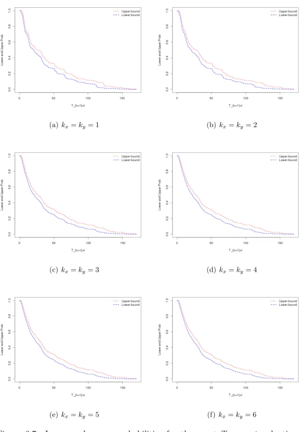
The lower and upper probabilities for the eventTn+1 > tare presented in Figure

2.6 only for the Normal copula, and Table 2.14 shows the NPI lower and upper probabilities for the event Tn+1 > t for different parametric copulas, for selected

(44)

2.6. Examples 35 values of t. These results can be used in a variety of ways, depending on the actual question of interest. From this table, we can see that the value of NPI lower and upper probabilities are different at each t among the parametric copulas. Figure 2.6 shows that the imprecision, which is the difference between corresponding upper and lower probabilities, is pretty similar through the main range of empirical values for xi +yi. This is due to the effect discussed for the simulations in Section 2.5,

namely the positive correlation between Loss and ALEA combined with interest in the sum of these quantities. If the data would have indicated a negative correlation, then imprecision would vary more substantially for the sum of the two quantities. In Figure 2.7, we show the imprecision for different parametric copulas considered. From this figure, we can see that imprecision is quite similar for these parametric copulas.