A Churn prediction model based on gaussian processes

Processes

by

Mehdi Ben Lazreg

supervised by

Ole-Christofer Granmo

Master Thesis in

Information and Communication Technology

The University of Agder, Faculty of Engineering and Science Department of Information and Communication Technology

Abstract

The telecommunication’s market has changed to a saturated one during the past few years. This makes it relatively costly to acquire new customers than to retain existing ones. Recent research has further showed that identifying potential cus-tomers who intend to leave a service provider for another (churners) and offering them an incentive to keep their subscriptions can produce significant savings for the telecommunication company. However, in most cases, it turned out that most of the used techniques to solve this problem fails to address the complex relation-ship between customer features and churn. Therefore, they struggle to achieve acceptable prediction accuracy. This might be due to the fact that real customers’ data are large, unbalanced, with missing values, and with non-linear dependen-cies between features. In this thesis, I investigated a new class of techniques for predicting customer churn based on Gaussian processes - a recent approach to re-gression and classification based on Bayesian reasoning principles. I developed a Gaussian process based model for churn prediction and tested it on a real cus-tomers’ data belonging to a French telecommunication’s company (Orange). The method obtained an area under the curve (AUC) score of 0.77. This score out-performed most of the previously used techniques that I evaluated on the same data set. The best of them had an AUC score of 0.73. To conclude, my empirical results proved that Gaussian processes can provide state-of-the-art performance in churn prediction, and the approach and results that I report offer a solid basis for further development of Gaussian processes for churn prediction.

This report is written in the context of IKT 590 Master thesis to fulfil a third semester requirement of master in information and communication technologies at the faculty of engineering and science at the University of Agder. The work on this project started on January 2013 under the supervision of professor Ole-Christofer Granmo. Since then I started studying the basic of Gaussian processes and how can we apply them to churn prediction. We were able to test our approach on a data set containing informations about the behaviour of a French telecommu-nication company’s costumers and I succeeded to obtained encouraging results. At the culmination of this work, I would like to take the opportunity to thank all those who helped me achieve the objectives of this thesis. I would also like to pay my gratitude to my project supervisor professor Ole-Christofer Granmo. His knowledge and experience of the field were remarkable. His guidance throughout the hole project, his precious technical advices and his directives and suggestions were crucial to the success of my work. Finally, I want to thank all the fellow stu-dents as well as the university’s personnel and teachers who helped me in multiple ways during all the course of my studies at the university of Agder.

Grimstad May, 2012

Contents

2 Review of previous works 5 3 A review of Gaussian process learning 8 3.1 Gaussian process . . . 9

3.2 Covariance function . . . 10

3.2.1 Stationary covariance function . . . 11

3.2.2 The dot product covariance function . . . 14

3.3 Gaussian Process regression . . . 17

3.4 Gaussian Process classification . . . 20

3.4.1 The Laplace approximation . . . 21

4 Churn prediction using Gaussian processes 24

4.1 Proposed solution . . . 24

4.2 Model selection . . . 26

4.3 Adaptation of hyperparameters . . . 26

5 Data preprocessing 29 5.1 Description of the data set . . . 29

5.2 Data preprocessing scheme . . . 30

5.3 Feature selection . . . 31

5.4 Data analysis . . . 32

6 Experiments and evaluation 36 6.1 Accuracy measurement criteria . . . 37

6.2 Experiments and discussion . . . 37

6.3 Evaluation of the results . . . 42

7 Conclusion and further work 46 7.1 Conclusion . . . 46

7.2 Further work . . . 47

A Mathematical background 48 A.1 Bessel function . . . 48

A.2 Concavity . . . 49

A.3 The exponential family of functions . . . 50

A.4 Kullback-Leibler divergence . . . 50

B Glossary and Abbreviation 51 B.1 Glossary . . . 51

B.2 Abbreviation . . . 52

List of Figures

1.1 Percentage of mobile phone subscriptions per 100 inhabitant in

different European countries in 2009 . . . 2

3.1 Example of a function generated by the Theγ-exponential kernel forγ = 0.5 . . . 11

3.2 Example of function generated by the squared exponential kernel . 12 3.3 Example of function generated exponential kernel . . . 13

3.4 Value taken by a piecewise polynomial kernel in function of r . . . 14

3.5 Example of a function generated by the The white noise kernel for σ = 1 . . . 15

3.6 Example of a set of function generated by dot product kernel . . . 15

3.7 Example of a Gaussian process regression . . . 18

4.1 Solution’s steps . . . 25

5.1 Date processing scheme . . . 31

5.2 Visual of the two of the most informative feature and their relation with the target value . . . 33

5.3 SOM presentation of the data . . . 34

5.4 2D Presentation of features 144 and 93 . . . 34

5.5 2D Presentation of features 51 and 93 . . . 35

6.1 Results of Gaussian process classification applied to all the data set 38 6.2 Results of Gaussian process classification applied with different

numbers of features . . . 39 6.3 Results of Gaussian process classification applied to the numerical

features . . . 40 6.4 Results of Gaussian process classification applied to the

categori-cal features . . . 41 6.5 Result of the combination of two Gaussian processes . . . 42 6.6 Result of the combination of two Gaussian processes with white

noise . . . 43 6.7 Example of decision tree learning tree for learning costumers’ churn 43

List of Tables

3.1 Summary of several commonly used covariance functions . . . 16

Introduction

Customers’ churn prediction is the term adopted to describe the process of iden-tifying customers who intend to quit a company and move to another service provider [8]. It has become, during the recent years, a relevant subject of data mining and has been investigated in different industries including banking [7] [19], life insurance [14] and telecommunication [22] [11] [10]....

Churning customers can be divided into two main groups: financial and com-mercial churners. In one hand, financial churn occurs when either the company or the customer unwillingly decides to cancel the subscription due to facts such as the customer can no longer afford to pay for the service. On the other hand, commercial churn takes place if the customers willingly decide to withdraw his subscription. This can be due to different reasons including that he or she found a cheaper offer in a concurrent company or realised that this latest disposes of a new technology that the original company does not have.... Although it is difficult to distinguish between the two categories just by looking at the company’s cus-tomers’ database. This is because they are mostly related to a privet aspect of the customer life, Burez and den Poel [3] made an attempt to differentiate between them in the case of a pay-TV company. They concluded that financial churn are easier to detect.

CHAPTER 1. INTRODUCTION

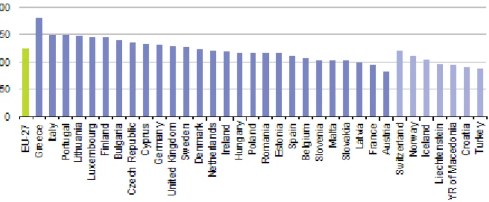
Figure 1.1: Percentage of mobile phone subscriptions per 100 inhabitant in differ-ent European countries in 2009

Source: Eurostat

1.1

Motivation

The telecommunication’s markets changed, in the last decade, from a fast growing market to a saturated one. For example, the average percentage of mobile phone subscription per 100 inhabitant is around 125% in the European union countries. It is around 110% in Norway (figure 1.1) which means that there are more phone subscriptions than inhabitant. This makes it more difficult to acquire new cus-tomers and pouches many telecommunication’s companies to try to focus more and more on retaining the existing ones. Moreover, Mozer et al. [15] showed that using predictive techniques to identifying potential churner and offer them an incentive to keep their subscriptions can produce significant savings for a telecom-munication company.

Another motivation to our work is the fact that Gaussian processes are a rich and powerful learning tool that allows to predict the likelihood of customers to churn. It has not been used previously to predict churn. This thesis will, then, be a small step in the direction of adapting Gaussian process to churn prediction.

1.2

Thesis’ objectives

In most cases, real customers’ data sets are large, unbalanced, with missing values, and non-linear dependencies between features. Furthermore, a combination of numerical and categorical features is typical. This makes churn prediction a chal-lenging data mining problem. Therefore, the first goal of this thesis is to work on the data-set by using some pre-processing techniques to deal with missing value as well as features’ selection. This treatment will allow a better performance for any machine learning algorithm [8].

Hadden et al. [8] also showed that state-of-the-art learning algorithm strug-gles to produce acceptable performance when applied to churn prediction. On the other hand, Gaussian processes learning is a rich technique that tries to predict the function that relates the features and the target value. It can handle more com-plex relationship between features and target function. Besides, Rasmussen and Williams [21] showed that under certain condition, techniques including logistic regression, neural network as well as support vector machines can considered as special case of Gaussian process.

Therefore, This thesis proposes to improve and adapt Gaussian processes to churn prediction. It will try to answer the question whether this method can out-perform most of the methods used in the field of churn prediction including lo-gistic regression, decision tree, neural networks.... Moreover, Gaussian process presents a fundamental parameter called covariance function that defines, in our case, when the algorithm considers two customers to have a similar behaviour. This thesis will investigate whether using different covariance function for differ-ent type of features can improve the result of the classification.

CHAPTER 1. INTRODUCTION

1.3

Contributions

The thesis will try to resolve the issue related to the data set. These issues include missing value, constant features and highly correlated features. It will propose a features selection technique based on the information gained by each feature about the target value. Besides, it will check a number of feature and their relation with the target value to discuss the difficulty of prediction churn based on these features.

Finally, it proposes Gaussian process as a novel approach for churn prediction. Gaussian processes are a reach and flexible method that deserves the investigation for this purpose. As it will be shown in chapter 2, Gaussian process were not used previously for churn prediction so I hope that this thesis will be a first and an encouraging step in that direction.

1.4

Thesis’ agenda

This report is arranged as follows: chapter 2 will present an overview of the pre-vious research done in the field of churn prediction.

Chapter 3 will introduce Gaussian process and how they can be used for re-gression and classification learning. Further chapter 4 will illustrate a solution to implement Gaussian process for churn prediction.

Chapter 5 presents a detailed description of steps followed to pre-process the data set and deal with its issues. A testing of the proposed approach on the pre-processed data will be performed in chapter 6. Farther, it will compare it with the other techniques developed for this purpose. The chapter will end by discussion whether the objectives describes in section 1.2 were answered.

The report will finally end by a conclusion summarising the main result of this thesis and proposing future work directions.

Review of previous works

Many research have been conducted over the years in order to predict customers’ churn. At first state of the art learning techniques has been investigated. Datta et al. [4] developed a churn analysis, modelling and prediction (CHAMP) model based on neural network. They used simple regression, nearest neighbour and decision trees as well. Nonetheless, their research could not distinguish a best method.

Hung et al. [10] also used decision tree and neural network to predict cus-tomers’ churn. They tried to evaluate the performance of each method by apply-ing them to detect the churners among the customers of a telecommunication’s company. Those methods were applied every month on a data set that was also monthly updated over a one-year period. Their result showed a height perfor-mance fluctuation due to the variation of the customers’ behaviour during that period and they could not establish a relationship between customer behaviour and the target value (churn in this case). Moreover, it should be acknowledged that the nature of a real-customers’ data set makes the problem really challenging for the state of the art machine learning techniques used in this case.

To address this problem, more advanced learning techniques started to be ex-plored. Hwang et al. [11] discovered that logistic regression performed better

CHAPTER 2. REVIEW OF PREVIOUS WORKS

than neural network and decision tree for churn prediction. However, it should be mentioned that they generated clusters of customers based on their past and future spendings. Then, they used those clusters as an input of the classification.

To deal with the non-linear dependency between feature, Yi and Guo-en [23] developed a support vector machine (SVM) model. SVM allows to model com-plex relationships between feature. It produces as output the likelihood of cus-tomers churn. The model outperformed logistic regression, neural network, deci-sion tree and Bayesian network when applied to predict churn for a telecommuni-cation’s company.

Au et al. [2] argued that beside knowing whether a customer is going to churn or not, it is important to discover the likelihood of the customers doing so. This allows the companies to target customer with a height churn probability by the mean of retention campaign. For this purpose, they developed a technique based on a combination of rules learning and genetic algorithms. The method outper-formed neural networks and decision tree.

Verbeke et al. [22] have developed a profit centric performance measure to evaluate customer churn prediction techniques. This method is based on the loss that a company can undergo if a misclassification occurs. For example, if a churner has been evaluated as non-churner, the company will not take action to retain him, he will then leave the company and the company will lose all the money that the customer would have spent if he stayed. Those losses are ac-cumulated and used as a measure for the classification techniques. Alternating decision tree (ADT a method based on combining different derision tree classifi-cation algorithms) and neural network has been distinguished from the other used classification techniques based on this criterion.

Furthermore, Niculescu-Mizil et al. [17] used the same data set that I have been able to get in the context of the knowledge discovery in data competition [5]. They used in the purpose of discovering churners a method based on ensem-ble selection. They started from a set of multiple classifiers, then, tried to found out which subset of those classifiers provides the better result. During this process

they also discovered that logistic regression provides the best individual result and combined with other classifiers can perform even better.

Mozer et al. [15], in the other hand, showed that a non-linear neural network outperformed logistic regression in prediction churn. They concluded that a so-phisticated non-linear neural network can better exploit non-linear structure in the data than a linear based logistic regression method. They also suggested as future research topic that using Gaussian process would help improve the prediction’s accuracy.

Finally, Gaussian processes has been used broadly for regression and classifi-cation problems that contain complex relationship between features and the target function [21]. It produced good result in robot dynamics learning [16], speech recognition [18] and human action recognition [24]. It has not been used for churn prediction. Nevertheless, SVM, neural network and logistic regression that proved to be good prediction techniques for churn as shown previously [15] [11] [23] are considered by Rasmussen and Williams [21] as special cases of Gaussian process under certain conditions. Rasmussen and Williams [21] further explains the rel-atively narrow use of Gaussian process by the fact that it requires handling large matrix and its inversion, which is a complex problem that need to be addressed especially for large data sets.

Chapter 3

A review of Gaussian process

learning

Supervised learning is a machine learning task that tries to infer a function from a labelled training data. Thus, given a set of observationD = {(xi, yi)|i= 1...n} where yi is a label associated to xi, supervised learning attempt to discover the functionf such that f(xi) = yi for all observations xi. In order to perform this task, some assumption must be made about the function f otherwise any func-tion that is consistent with the training data could be accepted. One way to do this would be to restrict the class of considered function by taking, for example, into account only linear functions. This approach could be limited especially if the labels and the observations are not linearly related. Another way would be to give a prior probability to each function where higher probabilities are assigned to functions that are considered more likely. This method, nonetheless, seems to have a serious problem since we are dealing with an infinite number of functions each one of them needs to be assigned a prior probability. This is where Gaussian process intervene.

This chapter will try to introduce Gaussian process (sections 3.1 and 3.2). Further, section 3.3 will present how it can be used for regression learning.

Fi-nally, section 3.4 will demonstrate how Gaussian process can be approximated and used for classification learning.

3.1

Gaussian process

Gaussian process is a generalisation of the Gaussian probability distribution. While a probability distribution describes a random variable which can be a scalar or a vector, a Gaussian process governs the properties of functions [21]. A set of func-tions is defined by simply defining a Gaussian process.

Definition 1 For any setS, a Gaussian process onSis a set of random variables

(f(t), t ∈S) such that∀n ∈ _N,∀t1...tn ∈ S(f(t1), ..., f(tn))is a multi-variant

Gaussian.

A Gaussian process is fully defined by its mean function:

µ(t) =_E[f(t)] (3.1) and its covariance or kernel function:

k(t, s) = _E[(f(t)−µ(t))(f(s)−µ(s))] (3.2) In the other hand:

Theorem 1 LetSbe a set,

µ:S →_Ra mean function and

k :S×S →_Ra covariance function

Then, There exists a Gaussian process(f(t))_t∈S such that:

CHAPTER 3. A REVIEW OF GAUSSIAN PROCESS LEARNING

The previous theorem states that a Gaussian process is simply generated by well defining a mean and a covariance functions. Thus, those two functions spec-ify a set of infinite function by the mean of that Gaussian process. Although the mean is important component of a Gaussian process it neither controls the shape nor the class of the function generated by the Gaussian process so it often taken as zero for simplicity reasons [21]. The covariance function on the other hand needs to be studied deeper.

3.2

Covariance function

The covariance function is the most important element of a Gaussian process. It encodes the assumption about the function that has to be learned[21]: It controls the shape and the nature of the function governed by the Gaussian process (contin-ued, discontinued...). From another perspective, the covariance function defines when two elements are considered similar, which is a critical aspect of supervised learning: if some set of elements having the same target value y are considered similar to another element x then it is more likely that x will have the same target value.

Definition 2 A covariance function is a functionk :S×S →_Rsuch that:

∀n∈_N;∀x1, ..., xn∈Sthe matrixC = (ci,j =k(xi, xj))is positive semi-definite

⇔ ∀u∈_Rn_;ut_Cu≥0

An infinity of functions can conform to the specification of the previous defi-nition. However, the most significant and used function can be organized into two categories [21].

3.2.1

Stationary covariance function

A stationary covariance function is a function of the difference r = x1 −x2 of

two valuex1 andx2 of a feature. These functions have the characteristic of being

invariant to any translation of the inputs. The most used stationary covariance function are:

Theγ-exponential covariance function: it has the following equation:

k(r) = exp−(r

l)

γ_{; 0< γ ≤2}

(3.3)

The parameterl defines a characteristic length-scale which controls what should be the minimum distance between x1 and x2 for them to be considered

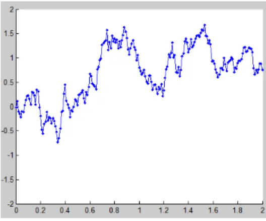
uncor-related. For large value of l, the covariance function will be independent of r. Figure 3.1 shows an example of a function generated by theγ-exponential kernel forγ = 0.5. It can be seen that for this value ofγ, the function generated by the Gaussian process is discontinued.

Figure 3.1: Example of a function generated by the Theγ-exponential kernel for

γ = 0.5

expo-CHAPTER 3. A REVIEW OF GAUSSIAN PROCESS LEARNING

nential covariance function. The kernel has the following expression:

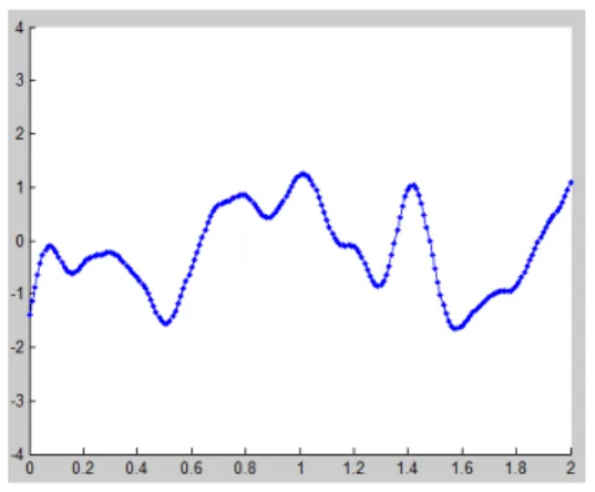
k(r) = exp −r 2 l2 (3.4)

It is the most famous covariance function. This function is infinitely differentiable which means that the functions generated by a Gaussian process with this covari-ance function is very smooth. An illustration of this is presented in figure 3.2.

Figure 3.2: Example of function generated by the squared exponential kernel

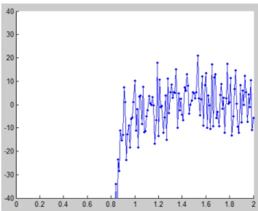
Another notable special case of this kernel is the case where γ = 1, the covari-ance function is called the exponential covaricovari-ance function. Figure 3.3 shows an example of a function generated by the exponential kernel. It can be seen that the function is discontinuous and had an exponential shape.

The Marten class of covariance functions: it has the following expression:

k(r) = 2 1−ν Γ(ν) √ 2νr l !ν Kν √ 2νr l ! (3.5)

WhereKν is a modified Bessel function (see A.1 for more detail),Γis the Euler gamma function andlis a free parameter of the covariance function. This process can model a less smoother or discontinues Gaussian processes. It should be noted

Figure 3.3: Example of function generated exponential kernel

the exponential covariance functions can also be obtained from this kernel when

ν = 1/2.

The rational quadratic covariance function: It has the following expression:

k(r) = 1 + r 2 2αl2 −α (3.6)

Whereαandlare free parameters. This function can be seen as the infinite sum of squared exponential covariance function with different length-scalelsince:

1 + r 2 2αl2 −α = Z h(l) exp −r2/2l2dl

Wherehis a given function.

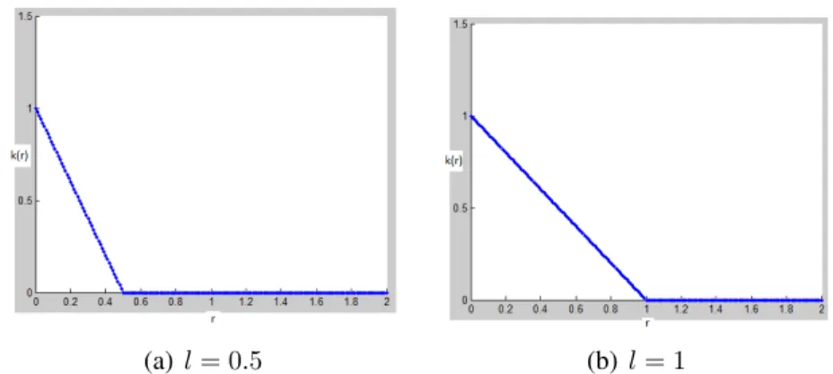
The piecewise polynomial covariance function: It has the following expres-sion:

k(r) =max(0,1− krk

l ) (3.7)

Where l is a free hyperparameter. The piecewise polynomial is a kernel with compact support which means that the covariance between two points will be

CHAPTER 3. A REVIEW OF GAUSSIAN PROCESS LEARNING

equal to zero if they distance exceeds a threshold specified by l. Figure 3.4 illustrate the value taken by a piecewise polynomial kernel as a function ofr for differentl.

(a)l= 0.5 (b) l= 1

Figure 3.4: Value taken by a piecewise polynomial kernel in function of r

White noise covariance function: it has the following expression:

k(r) = σδ(r) (3.8)

Whereδ is the Dirac delta function. Figure 3.5 shows an example of a function generated by the white noise kernel for σ = 1. The figure shows a randomly generated noise function centred around 0.

3.2.2

The dot product covariance function

The dot product covariance functions are a functions of the productx1x2 of two

value x1 andx2 of an input parameter. These function have the characteristic of

being invariant to rotation of the coordinate around the origin. They are mostly used to model a polynomial relationship between the features and the target value.

Figure 3.5: Example of a function generated by the The white noise kernel for

σ = 1

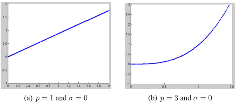
The most used dot product covariance function is:

k(r) = σ2₀+x1x2

p

;p∈_N (3.9)

Figure 3.6 shows the set of function generated by the covariance function of the previous equation for different choices ofp.

(a)p= 1andσ= 0 (b) p= 3andσ= 0

Figure 3.6: Example of a set of function generated by dot product kernel

Table 3.1 presents a summary of the most commonly used covariance func-tion. It should be noticed that each covariance function has a number free param-eters also known as hyperparamparam-eters. In the example of the squared exponential

CHAPTER 3. A REVIEW OF GAUSSIAN PROCESS LEARNING

Table 3.1: Summary of several commonly used covariance functions

Covariance function Expression Squared exponential exp−r2

2l2 Marten class 2_Γ(1−_νν₎ √ 2νr l ν Kν √ 2νr l Exponential exp −r l γ-exponential exp −(r_lγ) The rational quadratic 1 + ₂r_αl22

−α

piecewise polynomial max(0,1− kr_lk)

White noise σδ(r)

The dot product (σ2

0 +x1x2)

p

covariance function the hyperparemeter is l. In the case of the dot product co-variance function they areσandp. Those parameters need to be carefully chosen and can affect the accuracy of the predictive model. Section 4.2 will describe how those parameter are chosen in the case of churn prediction. Finally, it should be noted that other covariance functions can be obtained by combining the previ-ously cited functions following the subsequent propriety. The resulting function includes all the proprieties of the combined functions [21].

Propriety 1 Ifk1 andk2 are two covariance functions then the following func-tions are also covariance function:

• αk1;∀α ≥0

• k1+k2

3.3

Gaussian Process regression

We have seen in the beginning of this chapter that Gaussian process learning tries to identify the function that relates the features and the target value. To intuitively present this process, let us consider the simple case of one feature having different value for different instance. Each instance also have a target value. Figure 3.7(a) illustrates this scenario. The points in the figure correspond to the target value as function of the feature’s value for a given instances. Gaussian process regression tries to learn the most likely function that is consistent with those points. The shape and the nature (continued, discontinued, smooth...) of this function is con-trolled by the choice of the covariance function. This choice presents our prior knowledge about the function to be learned. It can be made by studying the data and discovering some patterns that could lead us to lean toward a certain kind of functions. Figures 3.7(b) and 3.7(c) illustrate the functions learned by two dif-ferent Gaussian process with difdif-ferent covariance functions (squared exponential in figure 3.7(b) and Marten class in figure 3.7(c)). It can be remarked that the function learned using the Marten class kernel is less smooth than the one learned using the squared exponential kernel. This due to the nature of the two kernel ex-plained in section 3.2.1. Finally, when the target valuet of a new instance needs to be learned, we just need to apply the learned function to the value of its feature

xlike presented in figures 3.7(d).

To put this into a more general and mathematical way, let us consider D =

{(x1, y1)...(xn, yn)} to be a data set where (xi)1≤i≤n ∈ Rd is the set of values taken by a number of features for a specific instance and(yi)1≤i≤n∈Rthe target value. In Gaussian process regression, we suppose that [21]:

yi =f(xi); 1 ≤i≤n (3.10) Where f(xi), xi ∈Rd

is a Gaussian process on_Rd_{. Further, let us assume} that this Gaussian process has a mean function µ and a covariance function k

CHAPTER 3. A REVIEW OF GAUSSIAN PROCESS LEARNING

(a) The target’s values as a function of the respective feature’s values

(b) Learned function using the squared exponential kernel

(c) Learned function using the Marten class kernel

(d) Learning the target value for a new instance

Figure 3.7: Example of a Gaussian process regression

and take an integer number p such that 0 < p < n. Moreover, Suppose that

yb = (yp+1, ..., yn)are the observed target value and that we want to infer ya = (y1, ..., yp).

In Gaussian process inference the problem is reduced to determine the probability

p(ya|yb).

Or equation 3.10 states thatyi =f(xi)and f(xi), xi ∈Rd

is a Gaussian process on_Rd_{so definition 1 gives that(f(x}

1), ..., f(xn))is a multi-variant Gaussian. This implies that Y = (y1, ..., yn) is also a multi-variant Gaussian (Y ∼ N(˜µ, K)) where:

˜ µ = (µ(x1), ..., µ(xn))t (3.11) K =       k(x1, x1) k(x1, x2) · · · k(x1, xn) k(x2, x1) k(x2, x2) · · · k(x,2xn) .. . ... . .. ... k(xn, x1) k(xn, x2) · · · k(xn, xn)       (3.12)

Let suppose that:

• µ˜= (µa, µb)twhere: – µa = (µ(x1), ..., µ(xp))t. – µb = (µ(xp+1), ..., µ(xn))t. • K = Ka,a Ka,b Kb,a Kb,b ! where: – Ka,a =     k(x1, x1) · · · k(x1, xp) .. . . .. ... k(xp, x1) · · · k(xp, xp)     . – Ka,b =     k(x1, xp+1) · · · k(x1, xn) .. . . .. ... k(xp, xp+1) · · · k(xp, xn)     . – Kb,a =     k(xp+1, x1) · · · k(xp+1, xp) .. . . .. ... k(xn, x1) · · · k(xn, xp)     . – Kb,b =     k(xp+1, xp+1) · · · k(xp+1, xn) .. . . .. ... k(xn, xp+1) · · · k(xn, xn)     .

CHAPTER 3. A REVIEW OF GAUSSIAN PROCESS LEARNING

Since Y = (ya, yb)is a multivariate Gaussian, then(ya|yb)is a multi-variant Gaussian [21](ya|yb)∼N(m, C)where:

m =µa+Ka,bKb,b−1(yb−µb) (3.13)

C =Ka,a−Ka,bKb,b−1Kb,a (3.14) Up to this point, we showed that the predictive distribution of the target valueya corresponding to a novel test inputs is a Gaussian with a mean and variance given respectively by equations 3.13 and 3.14. Once we computeK_b,b−1, calculating the mean and the variance is straightforward. However, when we are dealing with a big training set (over 10000 training sample [21]) computing K_b,b−1 becomes a resource and time-consuming problem. The purpose of this section was to present an application of Gaussian process to regression problem that we can use as an analogy to the classification problem.

3.4

Gaussian Process classification

In this section, we will discuss binary Gaussian process classification where target

yican take the value 1 or -1. The aim of the classification problem is to determine the probabilityp(ya|yb). In the regression problem, we supposed thatyi = f(xi) where f(xi), xi ∈Rd

is a Gaussian process on _Rd_{. Thus, f(x}

i) can take any value in_R. The basic idea of Gaussian classification is to turn the output of the regression model to a class probability by using a response function that squashes the output into the interval[0,1][21]. This grantees a valid probabilistic interpre-tation. An example of response function can be the logistic function:

σ(x) = 1

1 + exp(−x) (3.15)

yi =σ(f(xi)) (3.16) In Gaussian process regression, the set (f(x1), ..., f(xn)) is a multi-variant

Gaussian which allow us to get the result of equation 3.13 and 3.14. However, in the classification problem the set(σ(f(x1)), ..., σ(f(xn)))has a non-Gaussian likelihood, which makes the problem of determining p(ya|yb) intractable [21]. Hence, approximation method are used to approximate this distribution to a Gaus-sian distribution. This makes the computation of this likelihood less complex. The most used approximation methods are Laplace approximation and expecta-tion propagaexpecta-tion.

3.4.1

The Laplace approximation

The Laplace approximation is based on the second order Taylor expansion of lnp(ya|yb) around its maximum[21]. This maximum exists indeed (prove of its existence can be found in A.2). Lets supposed that it is obtained fory0 then, the

expansion would give:

ln(p(ya|yb)) = lnp(y0|yb) + 1 2∇∇ln(p(y0|yb))(ya−y0) 2 ⇒p(ya|yb) = exp(lnp(y0|yb)) exp( 1 2∇∇ln(p(y0|yb))(ya−y0) 2₎

LetF(y0) = lnp(y0|yb)and _σ12 =−∇∇lnp(y0|yb)then

p(ya|yb) = exp(F(y0)) exp(

1 2

(ya−y0)2

σ2 ) (3.17)

The probability distributionp(ya|yb)has an expression analogue to a Gaussian distribution with a meany0 and varianceσ2. Thus,ya|yb is locally approximated

CHAPTER 3. A REVIEW OF GAUSSIAN PROCESS LEARNING

to a Gaussian distribution∼N(y0, σ2).

3.4.2

The expectation propagation

The expectation propagation approximation starts from the fact that:

p(ya|yb) = p(yb|ya)p(ya) p(yb) = 1 p(yb) p(ya) n Y j=p+1 p(yj|ya) (3.18) Let g be a function such that:

   gp(ya) = p(ya) gj(ya) =p(yj|ya) Equation 3.18 gives: p(ya|yb) = 1 p(yb) n Y j=p gj(ya) (3.19) Wherep(yb) =R p(ya, yb)dya =R Qn_j=p+1gj(ya)dya.

By consequence, The hole problem comes down to determining the function

gj(ya)for allj.

The expectation propagation approximatesgj(ya)with a member of the expo-nential family of functions_egj(ya)[21](More detail about the exponential family of functions can be found in A.3). The result is a tractable functionq(ya) (equa-tion 3.20) that minimise an error metric betweenq(ya)and p(ya|yb). The error metric chosen in most cases is the Kullback-Leibler divergence (see A.4 for more detail)

q(ya) = 1 R Qn j=p+1egj(ya)dya n Y j=p+1 e gj(ya) (3.20) It should be noted that the expectation propagation approximation is a more sophisticated approach and has been proven to provide better results in practice that the Laplace approximation [21] since it chooses to proximate the posterior probabilityp(ya|yb)with a function that minimize an error metric. Whereas, the Laplace approximation locally approximate the posterior using a second order Taylor expansion. However, the expectation propagation is more complex and requires expensive computations compared to the Laplace method.

Chapter 4

Churn prediction using Gaussian

processes

After studying the basic aspect of Gaussian processes, this chapter will describe how can we use them on our data set to predict churn. In section 4.1, I will try to present an overview of the proposed solution. Chapter 3 proposed differ-ent types of covariance functions that can be used in Gaussian process learning. Each covariance function contains different parameters (referred to also as hyper-paramters) that need to be carefully chosen in order to build a accurate prediction model. Therefore, section 4.2 of this chapter will to explain the choice of the covariance functions and section 4.3 the choice of the hyperparamters.

4.1

Proposed solution

The data are composed of two types of features: numerical and categorical. Fur-thermore, we showed in section 3.2 that covariance function defines when two customers are considered having the same behaviour based on the values taken by the features for those customers. To further explain this point, let us suppose

that one of the numerical features is the number of call made by a customer and one of the categorical features contains the subscription type (prepaid, billed sub-scription,...). This latest is mapped to a number as we will see is section 5.3 with each number presenting a type of subscription. Lets now consider two customers with different number of calls made and different subscriptions’ type and that we are using a covariance function consisting on the difference between the value taken by each feature to discover how close the behaviour of those customers is. In the case of the numerical feature, the difference between the number of calls made can be a good criteria to distinguish between the two customers’ behaviours. However, In the case of the categorical feature, the difference between two ran-domly picked numbers representing the type of subscription would not hold a significant meaning and can, by consequence, harm the prediction process. But using a covariance function that takes the value zero if the customers have differ-ent subscription’s types and one otherwise can tell us if the two customers have the same subscription which could be a meaningful information.

Figure 4.1: Solution’s steps

I propose, then, as solution to the churn prediction problem to use different covariance functions for each type of features (numerical and categorical). Figure 4.1 shows the proposed solution. After the data processing, I spilt the data into two sets one containing the categorical feature and the other the numerical fea-tures. Then, I apply two Gaussian processes with different covariance functions to each type of feature. Since the result produced by each process is a churning probability, combining the results will consist on averaging the probabilities ob-tained from each one.

CHAPTER 4. CHURN PREDICTION USING GAUSSIAN PROCESSES

A final choice needs to be made concerning whether to use the Laplace ap-proximation or the expectation propagation apap-proximation in for the Gaussian process classification. Since the expectation propagation is a more sophisticated approach and has been proven to provide better results in practice that the Laplace approximation in many cases [21], I decided to use it for churn prediction.

4.2

Model selection

As seen in the previous section, the choice of the covariance function is an impor-tant issue. Therefore, a special care need to be taken to perform this choice. In the case of numerical features a stationary covariance function (section 3.2.1) can be the best choice. Nonetheless, the study of the data set that will be performed in chapter 5 did not provide any result that could lead to lean toward any of the covariance function. Consequently, in the experiments that will be done later, I will try different covariance functions and empirically discover the best one.

In the case of categorical features, as we discussed previously, the difference between the value of a feature would not have any significance. Thus, a function like the piecewise polynomial covariance function (section 3.2.1) that take the value 0 if the difference between the value of the feature exceeds a certain thresh-old could be a suitable choice if this latest is set to 1. In this case, if two customers have different feature’s values this function would return the value 0.

4.3

Adaptation of hyperparameters

We sow in section 3.2 that for a certain features the covariance function does not only depend on the values taken by that feature but also on a number of free parameters. For example, in the case of a squared exponential covariance function, we consider a feature taking the values x1 andx2 among others. The covariance

function can be expressed as follow: k(x1, x2) = exp −(x1−x2) 2 l2 (4.1)

Where the length-scale l represents the free parameter in this case. However, in our case we are dealing with a multitude of features and we want to apply the same covariance function -let’s say the squared exponential- to all of them. To solve this problem let us suppose the number of features to which we want to apply the same covariance function ism andxs and xt two vectors inRm. The elements of xs and xt represent the value taken respectively by each feature for two customer s andt. In this case, the squared exponential covariance function can be expressed as follows:

k(xs, xt) = exp −(xs−xt)tM(xs−xt)

(4.2)

Where M = diag(l₁−2, l−₂2, ..., l−_m2) is a diagonal matrix containing the value of different length-scale for each feature. The problem now is to find the value of M that best fits the data and the prediction we need to make. One approach could be to take different values of the elements ofMcorresponding to each feature. In this scenario, we are giving less importance to features assigned larger length-scale. Since, as seen in section 3.2.1, for large length-scale the covariance function will independent from that feature. This can be considered a kind of feature selection process. The other approach would be to take the same value for all the elements ofM. In this case, all the features will be considered having the same importance. However, for each case the hyperparameters need to be learned from the training set. To do so, let us consider in a more general case thatΘ = (Θ1,Θ2, ...,Θe)is a

vector containing all the hyperparamters of a covariance function k and we follow the notations of chapter 3 whereyb are the observed target. In the classification case,p(yb)is approximated to a multivariate GaussianN(µb, Kb,b)(section 3.4).

CHAPTER 4. CHURN PREDICTION USING GAUSSIAN PROCESSES where: Kb,b ≈     k(xp+1, xp+1) · · · k(xp+1, xn) .. . . .. ... k(xn, xp+1) · · · k(xn, xn)     ;µb = (µ(xp+1), µ(xp+2), ..., µ(xn)) Thus: p(yb) = 1 p (2π)b_|K b,b| exp −1 2(yb−µb) t_K−1 b,b(yb−µb) (4.3) ⇒lnp(yb) =− n−p 2 ln(2π)− 1 2ln(|Kb|)− 1 2(yb−µb) t_K−1 b (yb−µb) (4.4) SinceKb,b is a function ofΘ, the problem comes down the finding the value ofΘ that maximiselnp(yb). That implies findingΘ0 for which:

δ δΘlnp(yb) =− 1 2tr(K −1 b δKb δΘ) + 1 2(yb−µb) t_K−1 b δKb δΘK −1 b (yb−µb) = 0 (4.5) This approach allows to choose the hyperparamater that best fit the training data. However, it is likely that we are in a case with multiple local optima each one of them representing a different interpretation of the data and we end up choosing a value of Θcorresponding to one of local optima. Nonetheless, Rasmussen and Williams [21] states that choosing a value ofΘin a local optima does not highly affects the prediction’s accuracy.

Data preprocessing

In a case where the data set contains irrelevant, redundant or noisy data, the knowl-edge discovery process during the training phase becomes difficult. In this chapter, I will describe the first step of the solution presented in the previous chapter which data preprocessing. I will start by presenting an overview of the data set used for the classification (section 5.1). Section 5.3 demonstrate how the irrelevant fea-tures are filtered from the data. Finally, section 5.4 presents an analysis of the selected features. All the data procession done in this chapter were performed usingKNIMEa workbench for data mining and processing [1].

5.1

Description of the data set

The data set used in this thesis was provided by the French telecommunication company Orange in the context of the 2009 edition of the knowledge discovery in data competition (KDD cup 2009) [5]. The data contain 50000 instance and 230 features. It also includes a binary target variable corresponding to churn. The target takes the value 1 if the person is a churner and -1 otherwise. In addition to that the data set has the following characteristic:

CHAPTER 5. DATA PREPROCESSING

• A large number of missing values (about 60%).

• Unbalanced class proportions: the number of churners is much less then the number of non-churners (7.3% of the costumer in the data set are churners).

• Noisy data.

• A combination of numerical and categorical features (190 numerical fea-tures and 40 categorical feafea-tures).

For confidentiality reasons and to protect the privet information of its cus-tomers,Orangehas made the following modification on the data set:

• The features names were discarded and changed (the name of the features are henceforth: feature1, feature2,...,feature230).

• Multiplying each numerical feature by a random factor.

• Categorical features changed and mapped with randomly generated cate-gory names.

5.2

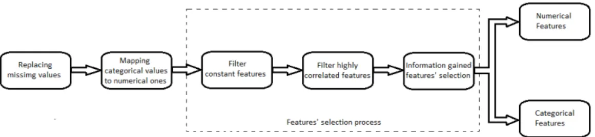
Data preprocessing scheme

Due to the proprieties of the data set illustrated in the previous section, some processing need to be done before carrying through any feature selection method. Figure 5.1 illustrates the different steps of the data processing. The first task was to replace the missing value. In the numerical features the missing numerical value were replaced with the average value of the feature in question. In the categorical feature, on the other hand, the missing value were replaced by the string ’missing’. Moreover, since Gaussian processes does not support learning for categorical features, I transformed all the strings in the categorical features to number using a bijective mapping between the set in a way that a string is represented by a unique number in the resulting data set.

Figure 5.1: Date processing scheme

5.3

Feature selection

Features’ selection consists on selecting from the data set the best set of features to use for the learning process. ’Different combinations of data hold different analytical powers’[8]. This means that depending on the prediction that need to be performed, a set of features that better fit this prediction have to be chosen. By consequence, it is necessary to identify the features that best suits the type of prediction to be carried through. In our case, the best features needed to perform costumers’ churn prediction have to be filtered. A special attention should be paid to feature selection because it helps reducing the amount of data to be used by keeping the important features and deleting the redundant and less informative ones. Moreover, the feature’s quality will influence the accuracy of the predictive model.

Then, I noticed that the data contain constant feature. So, I applied a filter that excludes the constant features from the data set. This operation reduced the number of features in the data set from 230 to 176.

Further, I applied a correlation filter to data set. This operation allows to fil-ter the redundant features. It consists on computing, for each pair of feature, a correlation coefficient that measures the correlation between two features. The computed coefficient is called the Pearson product-moment correlation coefficient (PCC). It is based on dividing the covariance between two feature by the product of their stander deviation. This coefficient is a number between -1 and 1, the closer this coefficient is to one the more correlated the features are. The features

CHAPTER 5. DATA PREPROCESSING

that have a PPC above a specific threshold are filtered. I set the threshold to 0.9 and this allowed to cut the number of features to 147.

Finally, in order to discover the worth of each feature and select the best ones to perform the classification, I applied a filter method to measure the information gained by each feature with respect to the target variable (In this case churn) [13]. It, then, orders the features from the more to the least important one by assign to each feature a weight representing the information gained.

The information gained is the change of information entropy between the tar-get variable and the tartar-get variable knowing the value of a specific feature is given. Let y be the target variable and x a features. The information gained is given by:

IG(y, x) = H(y)−H(y|x) (5.1) WhereH(y) =_E(−lnp(y))is the entropy ofy. This operation allows to discover that 88 of the previously selected 147 features bring near zero information about the target and are, then, eliminated. We are left with 59 features (41 numerical features and 18 categorical).

5.4

Data analysis

In this section, I will try to analyse some of the selected feature and their relation with each other and with the target value. First, I started with a look at the most in-formative of the features selected in the previous section. Figure 5.2 presents the number of occurrence of each value of feature51 and feature144 among the cus-tomers and the proportion of churning customer (in red) for each value. It should be noted by the look at the figure that those features -as well as the majority of the features in the data set- follow a Gaussian distribution with a small variance in feature144 and a larger one for feature52. We can also figure out why feature144 was one of the most informative feature: all the churner have the value 270 in this

feature.

(a) Feature51 (b) Feature144

Figure 5.2: Visual of the two of the most informative feature and their relation with the target value

Then, I tried to make a Self-organizing map (SOM) presentation of the data. It is a data exploring technique base on neural network. This technique is used to present on a two-dimensional space (called map) a highly dimensional instances of a data. SOM is composed of set of neurons, each neuron has an assigned weight, which is initialised to a small or random value. The input data is then fed to the neuron and the weight of each neuron is adjusted until it feats the input data [12]. At the end of the process each neuron will present a cluster of customers that are considered to have similar behaviour. This process will allow to verify if the selected features present any clear separation between the churners and the non-churners.

In the map (figure 5.3), The neuron are portrayed by pentagons and the circles inside each pentagon exhibit the cluster of customers represented by the neuron and the proportion of churner in each one. The darker the pentagon is the larger the distance between the customers represented by it and the ones represented by its neighbours. As the figure shows, a huge majority of the pentagons are white which means that, by looking at the features, no clear distinction exist between the cluster of customers represented by these pentagon and no clear border exist between the two categories of customers (churners and non-churners).

CHAPTER 5. DATA PREPROCESSING

Figure 5.3: SOM presentation of the data

Figure 5.4: 2D Presentation of features 144 and 93

Further, I tried to study the information that a combination of two feature can bring about the target value. For that purpose, I made a 2D plot representing a certain feature as a function of another. The results for different combination of feature is illustrated in figures 5.5, 5.6 and 5.4 where the red cross represent the churning customers and the blue cross the non-churning ones. As shown by the figures, no clear separation was discovered the two category of customers. In deed, the churning customers are scattered over all the possible values of the features.

Figure 5.5: 2D Presentation of features 51 and 93

Finally, the result of this section show that the correlation between the features and the target value is not important. This makes the problem of training for the data set and prediction the churning customers rather difficult.

Chapter 6

Experiments and evaluation

In this chapter, I will try to apply the Gaussian process classification on the data set after preprocessing. I used a Matlab implementation of Gaussian process de-veloped by Rasmussen and Nickisch [20]. During the experiments, I will test different choices of covariance functions and compared the results of the respec-tive predictions. In order to do that we need a better accuracy measurement criteria than the percentage of correct classification because -as we have seen in chapter 5- the data contain 7.3% churners. Thus, a classification algorithm that classifies all customers as non-churner will end up with 92.7% accuracy according to the percentage of correct classification criteria. That is a height score that does not reflect how poorly the algorithm performed. Section 6.1 will try to answer to this problem. Section 6.2 will expose and discuss the result obtained by Gaussian process classification. Finally, section 6.3 will try to compare those results to those of the previously used methods for churn prediction.

6.1

Accuracy measurement criteria

The percentage of correct classification metric does not constitute, as seen previ-ously, a proper accuracy measurement. The problem with that method arise when the churners are a minority in the data set. What we actually need is a criterion that would capture how many churners were detected by the classification algo-rithm.

The receiver operating characteristic (ROC) curve, on the other hand, is a graphical plot that allow to represent the true positive rate also known as sensitiv-ity (in our case the number of churning customers detected by the classification algorithm divided by the number of true churners) versus the false positive rate also known as specificity (in our case the number of churning customers not de-tected by the classification algorithm divide by the true number of non-churners). If the predictions are the churning probabilitypand we suppose that the customer is classified as churner ifp > S for0 < S < 1then the ROC curve present the sensitivity as a function of the specificity for each value ofS.

In this case, the area under the ROC curve (AUC) could be a good perfor-mance measure in our case since it allows to reduce the ROC curve perforperfor-mance to a single number representing the expected performance of the classification. A random method will have an identity line ROC cure with an AUC of 0.5. Classifi-cation algorithm are supposed to have AUC higher than this. The bigger the AUC is the higher the classification’ performance is.

6.2

Experiments and discussion

The data set contains 50000 customers. For the experiments, I divided it into two sets:

• Training set containing the third of data: this set is used to train the classi-fication algorithm and to evaluate the mean and the hyperparameters of the

CHAPTER 6. EXPERIMENTS AND EVALUATION

Figure 6.1: Results of Gaussian process classification applied to all the data set

covariance function.

• Testing set containing the rest of the data: this set is used to test the model build with the training set.

After the data preprocessing of chapter 5, we obtained a data set containing 59 fea-tures. In our first experiment we took the nine most informative ones containing a combination of numerical and categorical features (5 numerical and 4 categor-ical features) and tested the straightforward approach of applying the Gaussian process with different covariance functions. I tried the squared exponential (SE equation 3.4), Marten class (MC equation 3.5) and dot product (DP equation 3.9) covariance functions as well as the sum of MC and SE covariance functions and the sum of MC, SE and DP covariance functions. The result presented in fig-ure 6.1. The performance is rather poor with the best method having an AUC of 0.5384 with the SE kernel. We can also notice that summing the different

co-Figure 6.2: Results of Gaussian process classification applied with different num-bers of features

variance function did not have the effect of improving the results given by the SE kernel.

The next step was -as suggested in section 4.1- to separate the categorical and numerical features. However, I wanted to discover the optimal number of feature that I can use from the selected 59 of each type (categorical and numerical). To do that, I used the MC covariance function on a different number of numerical fea-tures. The results are presented in figure 6.2 where the best result was obtained with the five most informative numerical features with an AUC of 0.67. The same thing was done with the categorical feature using the piecewise polynomial co-variance function (PP equation 3.7) and the best result was obtained with the four most informative features.

Further, I used on the five numerical and four categorical features separately different covariance functions including the SE, MC, DP, and PP covariance func-tion. The performances are illustrated in figure 6.3 and 6.4. The result shows

CHAPTER 6. EXPERIMENTS AND EVALUATION

Figure 6.3: Results of Gaussian process classification applied to the numerical features

that the MC covariance function perform better with the numerical feature with an AUC of 0.67 and the PP covariance function provides a better accuracy with the categorical features with an AUC of 0.56. Each of those result is better than the result obtained in the first experiment (figure 6.1) where I used a Gaussian pro-cess classification on a combination of the same features. The best performance obtained so far is by Gaussian process applied on the numerical features alone. However, we can see that it struggles to make prediction out of the categorical features alone. This might be caused either by the possibility that Gaussian pro-cess leaning model is not suited to learning from categorical features or that the features themselves do not carry meaningful information about the target value.

The next step was to average the results giver by the Gaussian processes with the MC covariance function applied to numerical features alone and the PP co-variance function processes applied to categorical features alone. The results are illustrated in figure 6.5. The combination of the two Gaussian processes

Figure 6.4: Results of Gaussian process classification applied to the categorical features

(AUC=0.68) did not outperform by much the result obtained from the Gaussian process applied to numerical features alone. Nevertheless, it allowed to avoid the weak performance obtained by using a unique Gaussian process on all the features (figure 6.1) and surpass it by much. This result responds to the one of the research questions of this thesis namely: is using different Gaussian processes with distinct Kernels each on a different type of data could be beneficial for churn prediction? However, we still want to improve those results.

We have seen in chapter 5 that the data contain some noise. Therefore, in our next experience we tried to add a white covariance (WN equation 3.8) function to the MC and PP covariance functions used previously. This addition turned out to be highly beneficial as shows figure 6.6. The AUC was 0.77 and it was the best performance obtained during our experiment. Nonetheless, it still needs to be compared with other prediction’s methods to evaluate its worth.

CHAPTER 6. EXPERIMENTS AND EVALUATION

Figure 6.5: Result of the combination of two Gaussian processes

6.3

Evaluation of the results

In order to evaluate our result we tried to compare them with the results that most of the previously used methods for churn prediction obtained on our data set. Those methods are:

Decision tree learning: it is based on creating a decision tree (figure 6.7). Each node in the tree represent a feature. Based on the value of this feature for a specific customer a decision to choose the next node to move to is made. This process is repeated until the leaf node representing the class prediction is reached [13].

Alternating decision tree: it is a method based on combining different derision tree classification algorithms. In the case of decision tree learning in each node a decision is made based on the value of one feature. In the case of

Figure 6.6: Result of the combination of two Gaussian processes with white noise

Figure 6.7: Example of decision tree learning tree for learning costumers’ churn

alternating decision tree learning at each node the decision is made based on a vote between decision over multiple feature [6].

Artificial neural network: it is a set of entities called neurons that takes a set of input variables and tries to change it structure during the learning phase in order to find a relationship between the input variables and the target

CHAPTER 6. EXPERIMENTS AND EVALUATION

variable. Those relationships are used to predict the target variable [13].

Nave Bayesian classifier: it is based on the Bayesian theorem with the assump-tion that all the input variables or observaassump-tion{O1, O2, ..., On}are indepen-dent [13]. Lest assume that the target variable takes its value from the set

H ={h1, h2, ..., hm}. The nave Bayesian classifier tries to find the value of target variable that maximize the maximum a posteriori hypothesis:

Argmaxhj∈H(P(O1, O2, ..., On|hj)P(hj)) (6.1)

K nearest neighbour: it goes through a training data and, for each value of the target function, it label all the instances in the data set having this value with the same label. This procedure creates clusters of instances. It then goes ahead and measure the distance (in most cases Euclidean distance) between a new instance and all the cluster and find to which cluster it is the closest. The value of the target function that this cluster have is given to the new instance [13].

Logistic regression: it is based on the assumption the target valueyi is related to the values taken by the featuresxiby the relation [21]:

yi =

1 1 + exp(−xi)

(6.2)

Support vector machine(SVM): it is a special case of Gaussian process where the kernel is [21]:

K(xi, xj) = (xixj)d;d∈N (6.3) Ensemble selection: it is based on the idea that combining multiple predictive models could outperform any of those model used separately. In the ex-periments, I used a combination of random forests, boosted trees, logistic regression, SVM, decision trees, naive Bayes and KNN. This method was

Prediction method AUC Decision tree 0.54 Alternating decision tree 0.7 Artificial neural network 0.649

Nave Bayesian 0.644 K nearest neighbour 0.685 Logistic regression 0.696 Support vector machine 0.7

Ensemble selection 0.73

Table 6.1: Result of other prediction methods

the winning method of the KDD challenge from which we obtained our data set.

I used an implementation of those methods available in Knime[1] and Weka: a popular machine learning software developed in Java and containing a variety of learning algorithms[9]. The results of all those method are presented in table 6.1. The best of the alternative methods provides a performance of 0.73, but still not as good as the result obtained with our approach using Gaussian process. I should acknowledge that, for a lack of time, I did not go deep in the testing of those methods on the data set: I did not adapt their parameters to the problem in hand. Instead, I used a standard implementation of those methods. Moreover, I did not use a features selection process that select the best feature for each method. I rather used the most informative feature selected in chapter 5. This does not also mean that by using a feature selection process that adapt the selected features to each learning method we will end up with a totally different set of features. Thus, with more work, the result of the other tested method can be slightly improved and could be closer to the result obtained by the Gaussian process. This answer the question whether Gaussian process can outperform most of the method used in churn prediction, which is our second research question.

Chapter 7

Conclusion and further work

7.1

Conclusion

During this thesis, I studied Gaussian processes classification. Then, I investigate how can we use Gaussian process to predict customers churn. This allowed to develop a model for churn prediction based on separating the categorical and nu-merical features in the data set and use distinct Gaussian processes with different covariance functions on each.

The thesis started by processing the data to deal with missing value and irrel-evant features. Then, I used a feature selection technique that allows to discover which feature brings the most information about churn. Finally, I used previously described Gaussian process classification model. The best results were obtained using a Marten class of covariance function and piecewise polynomial covariance function -in addition to a white noise covariance function- respectively on numer-ical and categornumer-ical features. The performance was an AUC score of 0.77. These results outperformed a Gaussian process with those same covariance functions, but used on both types of features as well as most of the tested churn prediction techniques.

I hope that this work will be an encouraging step toward applying Gaus-sian process for churn prediction in the telecommunication’s industry and that it will motivate improving and enhancing this classification method and that it will broaden its use to may other areas.

7.2

Further work

The extension of this thesis can be done into two different directions. We can work on more data preprocessing that can help improve the results of the prediction. We can think of binning some rarely occurring value on certain features or work on combining exiting feature features to obtain new and more significant ones.

The second direction would be to work on the Gaussian process classification model itself. We have seen in chapter 6 that we did not obtain as good result with categorical as with numerical features and their combination did not improve by much the performance acquired by those latest. To improve this point, we can try to generate more sophisticated covariance functions that can capture better the relation between the features and the target value especially in the case of categorical features.

Appendix A

Mathematical background

A.1

Bessel function

A Bessel function is the solutiony(x)the Bessel differential equation:

x2d 2_y dx2 +x dy dx + (x 2₋ ν2)y= 0

The Bessel function of the first kind denoted asJν(x)are solution of the previous equation such that:

Jν(0) =c;c∈Rif ν >0 lim

x→0Jν(x) = 0if ν <0 (A.1)

Jν(x)can be expressed as follow:

Jν(x) = ∞ X m=0 (−1)m m!Γ(m+ν+ 1)( x 2) 2m+ν WhereΓ(x) = R∞ 0 t

x−1_e−t_{dtis the Euler gamma function. The modified Bessel} Bessel function has the following expression:

Kν(x) =

π

2

I−ν(x)−Iν(x) sin(νπ) WhereIν(x) =i−νJν(ix)andiis the imaginary unit.

A.2

Concavity

A functionf is concave if an only if its Hessian∇∇fis a negative definite matrix. on the other hand:

p(ya|yb) =

p(yb|ya)p(ya)

p(yb)

p(yb) does not depend of yi so proving that p(ya|yb) is concave comes down to proving that:∇∇lnp(yb|ya)p(yi = 1)is negative definite. Or:

lnp(yb|ya)p(ya) = lnp(yb|ya) + lnp(ya) and we know thatp(ya)is a multivariate Gaussian with:

p(ya) = 1 p (2π)a_|K a,a| exp −1 2y t aK −1 a,aya ⇒lnp(yb|ya)p(ya) = lnp(yb|ya)− a 2ln(2π)− 1 2ln(|Ka,a|)− 1 2y t aK −1 a,aya ∇lnp(yb|ya)p(ya) = ∇lnp(yb|ya)−Ka,a−1ya ∇∇lnp(yb|ya)p(ya) =∇∇lnp(yb|ya)−Ka,a−1 =−W −K −1 a,a

Where W = −∇∇lnp(yb|ya). Note that ∇∇lnp(yb|ya) is a diagonal matrix since yi does not depend on yj where j 6= i and yi = σ(f(xi)) so as long as we choose a log concave function σ, W will be positive definite. Since K−1

a,a is positive semi-definite by definition of a covariance matrix,∇∇lnp(yb|ya)p(ya)is a negative definite matrix andp(ya|yb)is concave. This shows that the maximum

APPENDIX A. MATHEMATICAL BACKGROUND

exists.

A.3

The exponential family of functions

A distribution from the exponential family of functions of function has the form:

fi(θ) = h(θ)g(η) exp(ηtu(θ))

Where η is a vector of hyperparameters. h, g and u are known functions. The normal distribution √ 1

(2πσ2₎exp

−(x₂−_σµ2)2

is a special case of the exponential family of functions where:

h(θ) = 1 2π η = ( µ σ2,− 1 2σ2) t g(η) = 1 |σ|exp(− µ2 2σ2) u(θ) = (θ, θ2)t

A.4

Kullback-Leibler divergence

Letpandpbe two probability density distribution such that:

• p+q = 1

• ifq(x) = 0thenp(x) = 0

Then the Kullback-Leibler divergence betweenpandpis defined as:

DLK(p||q) = Z

ln(p(x)

Glossary and Abbreviation

B.1

Glossary

∇: matrix differential Γ: Euler gamma function

µ: mean function

Θ: vector of hyperparameters D: data set

E: expected value of a random variable k: covariance function

Kν: modified Bessel function

N(m, C): multivariate Gaussian normal distribution with a mean mand covari-ance matrixC

p: probability distribution of a random variable S: random space

t: transpose of a matrix

xi: Set of observed features for a specific customer

APPENDIX B. GLOSSARY AND ABBREVIATION

B.2

Abbreviation

AUC: Area Under the Curve

CHAMP: CHurn Analysis, Modelling and Prediction DP: Dot Product

GP: Gaussian Process

KDD: Knowledge and Discovery on Data MC: Marten Class

PCC: Pearson product-moment Correlation Coefficient PP: Piecewise Polynomial

ROC: Receiver Operating Characteristic SE: Squared Exponential

SOM: Self-Organizing Map. SVM: Support Vector Machine WN: White noise