Classification of High Dimensional and Imbalanced
Hyperspectral Imagery Data
⋆V. Garc´ıa, J. Salvador S´anchez, and Ram´on A. Mollineda
Institute of New Imaging Technologies
Department of Computer Languages and Systems, Universitat Jaume I Av. Sos Baynat s/n, 12071
Castell´o de la Plana, Spain
{jimenezv,sanchez,mollined}@lsi.uji.es
Abstract. The present paper addresses the problem of the classification of hyper-spectral images with multiple imbalanced classes and very high dimensionality. Class imbalance is handled by resampling the data set, whereas PCA is applied to reduce the number of spectral bands. This is a preliminary study that pur-sues to investigate the benefits of using together these two techniques, and also to evaluate the application order that leads to the best classification performance. Experimental results demonstrate the significance of combining these preprocess-ing tools to improve the performance of hyperspectral imagery classification. Al-though it seems that the most effective order of application corresponds to first a resampling algorithm and then PCA, this is a question that still needs a much more thorough investigation.
1
Introduction
Hyperspectral sensors are characterized by a very high spectral resolution that usually results in hundreds of observation channels [22]. Although this allows to address many applications requiring very high discrimination capabilities in the spectral domain [3], the huge amount of data available makes complex the classification of hyperspectral images. In this classification context, another important drawback is that the hyperspec-tral information is commonly represented by a very large number of features (spechyperspec-tral bands), which are usually highly correlated [22, 23].
A complex situation frequently ignored in hyperspectral imaging refers to the pres-ence of severely skewed class priors. This situation is generally known as the class imbalance problem [12]. A data set is said to be imbalanced when one of the classes (the minority one) is heavily under-represented in comparison to the other (the major-ity) class. Because of samples of the minority and majority classes usually represent the presence and absence of rare cases respectively, they are also known as positive and negative examples. It has been observed that class imbalance often leads to poor classification performance in many real-world applications, especially for the minority classes.
⋆Partially supported by the Spanish Ministry of Education and Science under grants CSD2007– 00018, AYA2008–05965–0596–C04–04/ESP and TIN2009–14205–C04–04, and by Fundacio Caixa Castello–Bancaixa under grant P1–1B2009–04.
Most of the approaches to tackle the imbalance problem have been proposed both at the data and algorithmic levels. Data-driven methods consist of balancing the original data set, either by over-sampling the minority class [4,11] and/or by under-sampling [9, 17] the majority class until the classes are approximately equally represented. Within this group, we can also find several algorithms for feature selection [1, 15, 18, 25, 26]. At the algorithmic level, solutions include internally biasing the discrimination-based process [7, 8] and assigning distinct costs to the classification errors [19, 20, 30].
Although class imbalance has been extensively studied for binary classification problems, very few approaches deal with multi-class imbalanced data sets, as is the case of remote sensing applications. In the particular context of hyperspectral imagery, some proposals are adjustments of conventional learning algorithms [2,16,28], whereas others use classifier ensembles [24, 27] or feature selection techniques [5].
In this paper, some well-known strategies to cope with class imbalance are in-vestigated for the classification of hyperspectral imagery acquired by the Airborne Visible/Infrared Imaging Spectrometrer (AVIRIS1). The problem is of great relevance since these image data present both very high dimensionality and multiple imbalanced classes, what certainly provides additional challenges in the framework of remote sens-ing classification. In order to face such a problem, this work focuses on the joint use of feature extraction and resampling techniques, and explores the order in which they should be applied to achieve the best classification results.
The rest of the paper is organized as follows. Section 2 describes the methodology proposed to handle class imbalance and high dimensionality, and also briefly reviews the classifiers used in this work. Next, Sect. 3 contains the experiments on a real hy-perspectral image database and discusses the most important findings. Finally, Sect. 4 concludes the present study and outlines possible directions for future research.
2
Methodology
This section provides an overview of the method here proposed to handle and classify remote sensing data according to the two issues of interest previously pointed out. In a first stage, the hyperspectral image data set will be preprocessed with the double aim of balancing the skewed classes and reducing the number of features/bands, albeit not necessarily in this order. The second stage will consist of classifying the resulting set after overcoming those two problems. Note that only those algorithms that will be further used in the experiments are described in the present section.
2.1 Preprocessing
Taking the particular characteristics of hyperspectral data sets into account, most imag-ing tasks could usually benefit from the application of some preprocessimag-ing techniques. Here we concentrate on a common situtation in which the data set consists of multiple imbalanced classes in a high dimensional representation space.
Balancing the Classes Data level methods for balancing the classes consists of re-sampling the original data set, either by over-re-sampling the minority class or by under-sampling the majority class, until the classes are approximately equally represented. Both strategies can be applied in any learning system since they act as a preprocessing phase, thus allowing the system to receive the training instances as if they belonged to a well-balanced data set. By using this strategy, any bias of the learning system towards the majority class due to the skewed class priors will hopefully be eliminated.
The simplest method to increase the size of the minority class corresponds to ran-dom over-sampling, that is, a non-heuristic method that balances the class distribution through the random replication of positive examples. Nevertheless, since this method replicates existing examples in the minority class, overfitting is more likely to occur. Chawla et al. [4] proposed an over-sampling technique that generates new synthetic mi-nority samples by interpolating between several preexisting positive examples that lie close together. This method, called SMOTE (Synthetic Minority Over-sampling TEch-nique), allows the classifier to build larger decision regions that contain nearby samples from the minority class.
On the other hand, random under-sampling [14, 29] aims at balancing the data set through the random removal of negative examples. Despite its simplicity, it has em-pirically been shown to be one of the most effective resampling methods. Unlike the random approach, many other proposals are based on a more intelligent selection of the negative examples to be eliminated. For instance, the one-sided selection technique [17] selectively removes only those negative samples that either are redundant or that border the minority class examples (assuming that these bordering cases are noise).
Dimensionality Reduction The reduction in the hyperspectral representation space can be carried out by means of feature selection or extraction techniques. In both ap-proaches, the aim is to reduce the number of bands, without much loss of information. The process of feature selection is to choose a representative subset of features from the original data by assessing its discrimination capabilities according to statistical distance measures among classes (e.g., Bhattacharyya distance, Jeffries-Matusita distance, and the transformed divergence measure). The feature extraction approach addresses the problem of dimensionality reduction by projecting the data from the original feature space onto a low-dimensional subspace, which contains most of the original informa-tion [13].
Probably the most widely-known feature extraction method corresponds to Princi-pal Component Analysis (PCA), which seeks to reduce the dimension of the data by finding a few orthogonal linear combinations of the original variables with the largest variance. It involves a mathematical procedure that transforms a number of (possibly) correlated variables into a (smaller) number of uncorrelated variables called principal components.
2.2 Classification
We assume that there exists a set ofnpreviously labeled examples (training set, TS), say
xi and a class labelωi. Two traditional classification techniques will be used in the experimental study: the nearest neighbor rule and a decision tree.
Nearest Neighbor Rule One of the most popular non-parametric classification ap-proaches corresponds to theknearest neighbor (kNN) decision rule [6]. In brief, this classifier consists of assigning a new input samplexto the class most frequently rep-resented among thekclosest examples in the TS, according to a certain dissimilarity measure (e.g., the Euclidean distance). A particular case is whenk = 1, in which an input sample is decided to belong to the class indicated by its closest neighbor.
The characteristics of the kNN classifier need the entire TS stored in computer memory, what causes large time and memory requirements. On the other hand, the
kNN rule is extremely sensitive to the presence of noisy, atypical and/or erroneously labeled examples in the TS.
Decision Tree A decision-tree model is built by analyzing training data and the model is used to classify unseen data. The nodes of the tree evaluate the existence or signifi-cance of individual features. Following a path from the root to the leaves of the tree, a sequence of such tests is performed resulting in a decision about the appropriate class of new objects.
The decision trees are constructed in a top-down fashion by choosing the most ap-propriate attribute each time. An information-theoretic measure is used to evaluate fea-tures, which provides an indication of the ”classification power” of each feature. Once a feature is chosen, the training data are divided into subsets, corresponding to different values of the selected feature, and the process is repeated for each subset until a large proportion of the instances in each subset belongs to a single class.
3
Experiments and Results
The experiments were carried out on the 92AV3C data set2, which corresponds to a
hyperspectral image (145×145pixels) taken over Northwestern Indiana’s Indian Pines by the AVIRIS sensor in June 1992 and employed to recognize different land-cover classes. Although the AVIRIS sensor collects 224 spectral bands, four of these contain only zero values and so they can be removed, leaving a total of 220 non-zero bands. The ground truth data show that the image has 17 classes, although only 16 classes be-longing to different crop types, vegetation, man-made structures or other kinds of land were used (see Table 1). The omitted class contains unlabeled pixels, which presumably correspond to uninteresting regions or were too difficult to label.
In order to increase the statistical significance of the experimental results, classifi-cation accuracies were averaged over 30 different random partitions (2/3 of pixels for training and the rest for testing) of the original data set, preserving the prior class prob-abilities of each and the statistical independence between the training and test sets of every partition. The training sets were preprocessed by two different resampling algo-rithms, SMOTE and random under-sampling (RUS), to handle the class imbalance, and
Table 1.Number of training and test pixels per class, along with the relative percentage of sam-ples that belong to each class
Class Training Test %
1. Stone–steel towers 63 32 0.92 2. Hay–windrowed 326 163 4.72 3. Corn–min 556 278 8.05 4. Soybeans–notill 645 323 9.34 5. Alfalfa 36 18 0.52 6. Soybeans–clean 409 205 5.92 7. Grass/Pasture 331 166 4.79 8. Woods 863 431 12.48 9. Bldg–Grass–Trees—Drives 253 127 3.67 10. Grass/pasture–mowed 17 9 0.25 11. Corn 156 78 2.26 12. Oats 13 7 0.19 13. Corn–notill 956 478 13.83 14. Soybeans–min 1645 823 23.81 15. Grass/Trees 498 249 7.21 16. Wheat 141 71 2.05
also by PCA for dimensionality reduction by retaining those principal components with a variance of0.95. Because of difficulty to determine which classes to resample, we divided the biggest class (Soybeans–min) into four blocks (each one with 25% of sam-ples). Based on this, the remaining classes were over-sampled to reach 25%, 50% and 75% the size of the majority class. Similarly, the under-sampling was applied removing 25%, 50% and 75% of samples according to the size of the biggest class.
The J48 decision tree (an open source Java implementation of the very popular C4.5 algorithm) and the 1NN classifier were applied to sets that were preprocessed and also to each original training set (without any preprocessing). All hyper-parameters of the classifiers were set to the default values suggested in the WEKA toolkit [10]. Apart from calculating the average accuracy of each individual class to evaluate the effect of the preprocessing techniques on the majority and minority classes separately, the mean of these individual accuracies was also computed in order to have an overall estimate of the performance. For the sake of clarity, we averaged the three percentages of resampling (25%, 50% and 75%) in one single result.
3.1 Analysis of Results
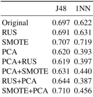
Table 2 reports the mean of the accuracies measured separately on each class when using J48 and 1NN to classify the test samples. As can be seen, the use of PCA (in-dividually or jointly with some resampling algorithm) produces an important decrease in 1NN performance, whereas both resampling techniques outperform the accuracies achieved on the original set. These results are much less significant with the decision tree. In the case of the 1NN classifier, PCA probably fails because the database here used includes noisy bands due to the effect of atmospheric absorption [21, 22]. It is
known that thekNN classifiers are very sensitive to noise in the training set and thus, the 1NN classifier seems to require a previous step consisting of the removal of those noisy bands or the application of some editing/filtering algorithm.
It is also remarkable that SMOTE excels all the other approaches, irrespective of the classifier used. On the other hand, when comparing the different combinations of resampling and PCA, one can observe that the application of SMOTE and PCA in this order leads to the highest performance in terms of mean of the accuracy of each class. Note that the average number of bands given by PCA is 13 in all cases, that is, it obtains a very high dimensionality reduction.
Table 2.Mean of accuracies of the 16 classes J48 1NN Original 0.697 0.622 RUS 0.691 0.631 SMOTE 0.707 0.719 PCA 0.620 0.393 PCA+RUS 0.619 0.397 PCA+SMOTE 0.631 0.440 RUS+PCA 0.644 0.387 SMOTE+PCA 0.710 0.456
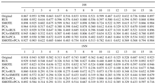
In order to assess the effect of the preprocessing approaches on each class sepa-rately, Table 3 shows the average classification accuracy achieved for each individual class. Both resampling techniques consistently improve the accuracy of the classes with less than 1% of samples (1, 5, 10, and 12), but entail a slight reduction on the perfor-mance of the most represented classes (8, 13, and 14). It is worth noting that this degra-dation on the majority classes appears to be less significant when using SMOTE, what is in keeping with the mean of accuracies reported in Table 2.
If we focus on the results of PCA, it is interesting to note that this algorithm leads to a decrease in the performance of most classes, especially when used with the 1NN clas-sifier. Surprisingly, the application of SMOTE before using PCA mitigates this effect, suggesting that it is important to balance the classes before reducing the dimensionality of hyperspectral data.
4
Conclusions and Further Extensions
The present paper has focused on classification of hyperspectral imagery with two com-plex characteristics: high dimensionality and severe skewed class distributions. The ex-perimental study has allowed to draw some preliminary conclusions: (i) It results more important to balance the classes rather than reduce the dimensionality, at least in terms of accuracy; (ii) The best choice seems to be the application of SMOTE followed by PCA; and (iii) The J48 decision tree appears to be a more robust classifier than the 1NN for this particular hyperspectral database.
Table 3.Average classification accuracy on each class J48 1 2 3 4 5 6 7 8 9 10 11 12 13 14 15 16 Original 0.867 0.953 0.598 0.663 0.637 0.516 0.833 0.916 0.521 0.599 0.467 0.432 0.632 0.736 0.884 0.897 RUS 0.888 0.952 0.616 0.677 0.596 0.576 0.843 0.880 0.556 0.597 0.500 0.412 0.594 0.593 0.868 0.904 SMOTE 0.898 0.925 0.602 0.675 0.599 0.561 0.827 0.898 0.580 0.724 0.522 0.395 0.615 0.717 0.866 0.904 PCA 0.964 0.918 0.517 0.627 0.380 0.398 0.642 0.878 0.360 0.612 0.416 0.329 0.515 0.670 0.840 0.891 PCA+RUS 0.923 0.929 0.538 0.647 0.386 0.469 0.685 0.824 0.396 0.640 0.427 0.310 0.487 0.521 0.818 0.896 PCA+SMOTE 0.945 0.863 0.532 0.631 0.507 0.440 0.681 0.806 0.457 0.634 0.521 0.304 0.481 0.642 0.760 0.895 RUS+PCA 0.905 0.930 0.580 0.672 0.419 0.490 0.703 0.836 0.402 0.653 0.463 0.464 0.529 0.534 0.822 0.902 SMOTE+PCA 0.927 0.903 0.622 0.685 0.664 0.483 0.754 0.834 0.513 0.782 0.611 0.652 0.569 0.568 0.794 0.904 1NN 1 2 3 4 5 6 7 8 9 10 11 12 13 14 15 16 Original 0.918 0.943 0.505 0.582 0.313 0.457 0.743 0.887 0.362 0.462 0.413 0.325 0.528 0.687 0.912 0.923 RUS 0.929 0.945 0.548 0.647 0.326 0.541 0.788 0.827 0.404 0.440 0.469 0.366 0.514 0.539 0.892 0.927 SMOTE 0.957 0.823 0.554 0.636 0.722 0.551 0.832 0.747 0.524 0.800 0.682 0.839 0.470 0.597 0.830 0.946 PCA 0.854 0.814 0.238 0.275 0.111 0.199 0.367 0.773 0.236 0.075 0.127 0.100 0.365 0.514 0.677 0.566 PCA+RUS 0.860 0.818 0.291 0.334 0.108 0.275 0.440 0.672 0.271 0.073 0.170 0.103 0.348 0.334 0.652 0.599 PCA+SMOTE 0.892 0.572 0.267 0.294 0.328 0.247 0.433 0.652 0.319 0.384 0.283 0.358 0.325 0.444 0.569 0.679 RUS+PCA 0.859 0.826 0.277 0.325 0.116 0.263 0.413 0.661 0.253 0.066 0.164 0.094 0.331 0.331 0.643 0.569 SMOTE+PCA 0.892 0.584 0.314 0.291 0.331 0.255 0.514 0.667 0.319 0.353 0.312 0.385 0.329 0.433 0.597 0.716
In hyperspectral imaging, selection is generally preferable to feature extraction be-cause of two main reasons. On the one hand, feature extraction would need the whole (or most) of the original data representation to extract the new features, forcing to al-ways deal with the whole initial representation of the data. Besides, since the data are transformed, some crucial and critical information might be compromised and distorted. Thus future research will be addressed to use some feature selection algorithm instead of PCA. Another direction for future studies would be incorporating an editing/filtering phase to remove possible noisy data before any other process.
References
1. Blagus, R., Lusa, L.: Class prediction for high-dimensional class-imbalanced data. Bioinfor-matics 11(1), 523–540 (2010)
2. Bruzzone, L., Serpico, S.B.: Classification of imbalanced remote-sensing data by neural net-works. Pattern Recogn. Lett. 18(11-13), 1323–1328 (1997)
3. Camps-Valls, G.: Machine learning in remote sensing data processing. In: Proc. IEEE Int’l. Workshop Machine Learning for Signal Processing. pp. 1–6. Grenoble, France (2009) 4. Chawla, N., Bowyer, K., Hall, L., Kegelmeyer, W.: SMOTE: Synthetic minority
over-sampling technique. J. Artif. Intell. Res. 16, 321–357 (2002)
5. Chen, X., Fang, T., Huo, H., Li, D.: Semisupervised feature selection for unbalanced sample sets of VHR images. IEEE Geosci. Remote Sens. Lett. 7(4), 781 –785 (2010)
6. Cover, T., Hart, P.: Nearest neighbor pattern classification. IEEE Trans. Inf. Theory 13(1), 21–27 (1967)
7. Ezawa, K., Singh, M., Norton, S.: Learning goal oriented bayesian networks for telecom-munications risk management. In: Proc. 13th Int’. Conf. Machine Learning. pp. 139–147 (1996)
8. Fawcett, T., Provost, F.: Adaptive fraud detection. Data Min. Knowl. Disc. 1(3), 291–316 (1997)
9. Garc´ıa, S., Herrera, F.: Evolutionary undersampling for classification with imbalanced datasets: Proposals and taxonomy. Evol. Comput. 17(3), 275–306 (2009)
10. Hall, M., Frank, E., Holmes, G., Pfahringer, B., Reutemann, P., Witten, I.: The WEKA data mining software: an update. SIGKDD Explor. Newslett. 11, 10–18 (2009)
11. Han, H., Wang, W.Y., Mao, B.H.: Borderline-SMOTE: A new over-sampling method in imbalanced data sets learning. In: Proc. Int’l. Conf. Intelligent Computing. pp. 878–887. Hefei, China (2005)
12. He, H., Garcia, E.: Learning from imbalanced data. IEEE Trans. Knowl. Data Eng. 21(9), 1263–1284 (2009)
13. Hsu, P.H., Tseng, Y.H., Gong, P.: Dimension reduction of hyperspectral images for classifi-cation appliclassifi-cations. Geogr. Inf. Sci. 8(1), 1–8 (2002)
14. Japkowicz, N., Stephen, S.: The class imbalance problem: A systematic study. Intell. Data Anal. 6(5), 429–449 (2002)
15. Kamal, A., Zhu, X., Narayanan, R.: Gene selection for microarray expression data with im-balanced sample distributions. In: Proc. Int’l. Joint Conf. Bioinformatics, Systems Biology and Intelligent Computing. pp. 3–9. Shanghai, China (2009)
16. Kubat, M., Holte, R., Matwin, S.: Machine learning for the detection of oil spills in satellite radar images. Mach. Learn. 30(2-3), 195–215 (1998)
17. Kubat, M., Matwin, S.: Addressing the curse of imbalanced training sets: One-sided selec-tion. In: Proc. 14th Int’l. Conf. Machine Learning. pp. 179–186. Nashville, USA (1997) 18. Lin, L., Ravitz, G., Shyu, M.L., Chen, S.C.: Effective feature space reduction with
imbal-anced data for semantic concept detection. In: Proc. Int’l. Conf. Sensor Networks, Ubiqui-tous, and Trustworthy Computing. pp. 262–269. Taichung, Taiwan (2008)
19. Liu, X.Y., Zhou, Z.H.: The influence of class imbalance on cost-sensitive learning: An em-pirical study. In: Proc. 6th Int’l. Conf. Data Mining. pp. 970–974. Hong Kong (2006) 20. Maloof, M.: Learning when data sets are imbalanced and when costs are unequal and
un-known. In: Workshop Learning from Imbalanced Data Sets II. Whasington, DC (2003) 21. Mart´ınez-Us´o, A., Pla, F., Sotoca, J.M., Garc´ıa-Sevilla, P.: Clustering-based hyperspectral
band selection using information measures. IEEE Trans. Geosci. Remote Sens. 45(12), 4158–4171 (2007)
22. Melgani, F., Bruzzone, L.: Classification of hyperspectral remote sensing images with sup-port vector machines. IEEE Trans. Geosci. Remote Sens. 42(8), 1778–1790 (2004) 23. Richards, J., Jia, X.: Using suitable neighbors to augment the training set in hyperspectral
maximum likelihood classification. IEEE Geosci. Remote Sens. Lett. 5(4), 774–777 (2008) 24. Trebar, M., Steele, N.: Application of distributed SVM architectures in classifying forest
data cover types. Comput. Electron. Agr. 63(2), 119–130 (2008)
25. Van Hulse, J., Khoshgoftaar, T., Napolitano, A., Wald, R.: Feature selection with high-dimensional imbalanced data. In: IEEE Int’l. Conf. Data Mining Workshops, 2009. pp. 507– 514. Miami, USA (2009)
26. Wasikowski, M., Chen, X.W.: Combating the small sample class imbalance problem using feature selection. IEEE Trans. Knowl. Data Eng. 22(10), 1388–1400 (2010)
27. Waske, B., Benediktsson, J.A., Sveinsson, J.R.: Classifying remote sensing data with sup-port vector machines and imbalanced training data. In: Proc. 8th Int’l. Workshop Multiple Classifier Systems. pp. 375–384. Reykjavik, Iceland (2009)
28. Williams, D., Myers, V., Silvious, M.: Mine classification with imbalanced data. IEEE Geosci. Remote Sens. Lett. 6(3), 528 –532 (2009)
29. Zhang, J., Mani, I.: kNN approach to unbalanced data distributions: a case study involving information extraction. In: Proc. Workshop Learning from Imbalanced Datasets. Washington DC (2003)
30. Zhou, Z.H., Liu, X.Y.: Training cost-sensitive neural networks with methods addressing the class imbalance problem. IEEE Trans. Knowl. Data Eng. 18(1), 63–77 (2006)