Transport Services. Data v2.0 (2007)

(1)

Swiss Centre

for Life Cycle

Inventories

A joint initiative of the ETH domain and Swiss Federal Offices

Transport Services

Data v2.0 (2007)

Michael Spielmann

Christian Bauer

Roberto Dones

Paul Scherrer Institut, Villigen

Matthias Tuchschmid

ESU-services Ltd., Uster

ecoinvent report No. 14

(2)

Project "ecoinvent data v2.0"

Commissioners: Swiss Centre for Life Cycle Inventories,

Dübendorf

Swiss Federal Office for the Environment (BAFU - FOEN), Bern

Swiss Federal Office for Energy (BFE), Bern Swiss Federal Office for Agriculture (BLW), Bern

ecoinvent Board: Alexander Wokaun (Chair) PSI, Villigen

Gérard Gaillard, Agroscope Reckenholz-Tänikon Research Station, ART, Zürich

Lorenz Hilty, Empa, St. Gallen Konrad Hungerbühler, ETHZ, Zürich François Maréchal, EPFL, Lausanne

ecoinvent Advisory Council: Norbert Egli, BAFU, Bern

Mark Goedkoop, PRé Consultants B.V. Patrick Hofstetter, WWF, Zürich

Roland Högger, öbu / Geberit AG, Rapperswil Christoph Rentsch, BAFU (until January 2006) Mark Zimmermann, BFE (until July 2007)

Institutes of the ecoinvent Centre:

Swiss Federal Institute of Technology Zürich (ETHZ)

Swiss Federal Institute of Technology Lausanne (EPFL)

Paul Scherrer Institute (PSI)

Swiss Federal Laboratories for Materials Testing and Research (Empa)

Agroscope Reckenholz-Tänikon Research Station (ART)

Participating consultants: Basler & Hofmann, Zürich

Bau- und Umweltchemie, Zürich Carbotech AG, Basel

Chudacoff Oekoscience, Zürich Doka Life Cycle Assessments, Zürich

Dr. Werner Environment & Development, Zürich Ecointesys - Life Cycle Systems Sarl.

ENERS Energy Concept, Lausanne ESU-services Ltd., Uster

Infras AG, Bern

Software Support: ifu Hamburg GmbH

Project leader: Rolf Frischknecht, ecoinvent Centre, Empa,

Dübendorf

Marketing and Sales: Annette Köhler, ecoinvent Centre, Empa,

(3)

Citation:

Spielmann, M., Bauer, C., Dones, R., Tuchschmid, M. (2007) Transport Services. e-coinvent report No. 14. Swiss Centre for Life Cycle Inventories, Dübendorf, 2007

Transport Services

Authors 2007, v2.0: Michael Spielmann, Christian Bauer, Roberto

Dones, Matthias Tuchschmid

Authors 2003, 2004: Michael Spielmann, ETHZ-UNS

Thomas Kägi, ETHZ-UNS Philipp Stadler, ETHZ-UNS

Reviewer: Thomas Kägi, Agroscope Reckenholz-Tänikon

Research Station (ART) (2007) Niels Jungbluth (2003, 2004, 2007)

Contact address: ecoinvent Centre

Empa

P.O. Box

CH-8600 Dübendorf

http://www.ecoinvent.org/ [email protected]

Responsibility: This report has been prepared on behalf of one or

several Federal Offices listed on the opposite page (see commissioners) and / or the ecoinvent Centre. The final responsibility for contents and conclusions remains with the authors of this report.

Terms of Use: Data published in this report are subject to the

ecoinvent terms of use, in particular paragraphs 4 and 8. The ecoinvent terms of use (Version 2.0) can be downloaded via the Internet

(www.ecoinvent.org).

Liability: Information contained herein have been compiled

or arrived from sources believed to be reliable. Nevertheless, the authors or their organizations do not accept liability for any loss or damage arising from the use thereof. Using the given information is strictly your own responsibility.

(4)

(5)

Acknowledgement ecoinvent v2.0

The author would like to thank, Natascha Kljun and Christoph Schreyer (INFRAS) and Bart Van Her-bruggen (Transport & Mobility Leuven) for providing background information and knowledge. Also, we thank Thomas Kägi for the review of the report and original data files.

Acknowledgement ecoinvent v1.0

Our thanks go to the reviewer Niels Jungbluth from ESU-services for his useful comments.

We would also like to thank Prof. Dr. Roland W. Scholz and Peter de Haan (ETH-NSSI) for their su-pervision of the work.

The following individuals contributed to the study by providing data, information or expert knowl-edge, or by helping in other ways:

G. Doka, Doka Ökobilanzen, Zürich Switzerland.. R. Dones and Th. Heck, PSI, Villigen, Switzerland. R. Frischknecht, ESU-Services, Uster, Switzerland.. A. Giannouli, Aristotle University of Thessaloniki..

M. Halder and H. Schwarz und Deutsche Bahn AG, Bahn Umweltzentrum, Berlin. R. Hischier, EMPA, St. Gallen.

H.J. Althaus und D. Kellenberger, EMPA, Dübbendorf, Switzerland H. Jenk, BUWAL, Bern, Switzerland..

M. Keller and P. de Haan, INFRAS-Bern, Switzerland. W. Knörr, Ifeu-Heidelberg, Germany..

H. Kuppelwieser, SBB, Bahn Umweltzentrum, Bern, Switzerland.. D. Peter and C. Schreyer, INFRAS-Zürich, Switzerland.

W. Schweimer, Volkswagen AG, Wolfsburg, Germany.. H. Stram, Masterplanung, uniqueairport, Zürich, Switzerland.. S. Stühler, MAN-Nutzfahrzeuge AG, München, Germany

(6)

Summary

Freight transport occurs between nearly any two process steps of a product system and often is of ma-jor importance for a product life cycle. In addition, passenger transport services e.g. for business and service trips are of growing interest for Life Cycle Assessment studies. Comprehensive life cycle in-ventories (LCI) of various means of transport are available from Frischknecht (1996)and Maibach (1999). Within the framework of ecoinvent 2000 projects, these data have been extended, updated and harmonised.

The main objective of transport modelling in ecoinvent is to provide background data for transport services in order to complete a variety of product life cycles. Generic background data have been gen-erated for four modes of transport (air-, rail-, road- and water transport) to account for environmental interventions due to the transportation between two process steps of a product system. The data repre-sent average transport conditions in Switzerland and Europe.

In order to quantify environmental exchanges of transport services and relate transport datasets to other product life cycles, the environmental exchanges are related to the reference unit of one tonne kilometre [tkm]. A tonne kilometre is defined as the transport of one tonne of goods by a certain trans-port service over one kilometre. Passenger transtrans-port data is expressed in passenger kilometres [pkm]. Each mode of transport is further separated into sub-groups, referred to as transport services, using several criteria such as geographical operation (e.g., rail transport), vehicle size (e.g., road transport) and transported goods (e.g., water transport). Transport services are divided into several datasets, so-called transport components. In addition to vehicle operation (comprising vehicle travel and pre-combustion), infrastructure processes such as vehicle maintenance, manufacturing and disposal as well as transport infrastructure construction, operation and disposal are also modelled.

(7)

New and Updated Transport Datasets in ecoinvent v2.0

The ecoinvent data v2.0 contain new and updated life cycle inventories of transport systems based on fossil fuels and biofuels as well as life cycle inventories of electric railway transport systems. This re-port contains the inventories and documentation of fossil fuel-based and railway transre-port services, while biofuel-based transport services are documented in (Jungbluth et al. 2007).

Fossil fuel-based and railway transport services

Comprehensive life cycle inventories (LCI) for various transport services (road, rail, water and air) have been produced within the framework of ecoinvent v1.1 by Spielmann (2004). Within the frame-work of ecoinvent v2.0, data the focus is the extension and update of road transport datasets. In addi-tion the figures for Swiss rail transport have been updated and some datasets representing the rail transport of coal in China and the USA have been added.

In the tables below the updated and new datasets are presented.

Tab. 1: Datasets for Freight Transport Services in Europe (RER)

Dataset name Location Category Sub-Category Unit Status

operation, lorry 3.5-7.5t, EURO3 RER transport systems road vkm new operation, lorry 3.5-7.5t, EURO4 RER transport systems road vkm new operation, lorry 3.5-7.5t, EURO5 RER transport systems road vkm new operation, lorry 7.5-16t, EURO3 RER transport systems road vkm new operation, lorry 7.5-16t, EURO4 RER transport systems road vkm new operation, lorry 7.5-16t, EURO5 RER transport systems road vkm new operation, lorry 16-32t, EURO3 RER transport systems road vkm new operation, lorry 16-32t, EURO4 RER transport systems road vkm new operation, lorry 16-32t, EURO5 RER transport systems road vkm new operation, lorry >32t, EURO3 RER transport systems road vkm new operation, lorry >32t, EURO4 RER transport systems road vkm new operation, lorry >32t, EURO5 RER transport systems road vkm new transport, lorry 3.5-7.5t, EURO3 RER transport systems road tkm new transport, lorry 3.5-7.5t, EURO4 RER transport systems road tkm new transport, lorry 3.5-7.5t, EURO5 RER transport systems road tkm new transport, lorry 7.5-16t, EURO3 RER transport systems road tkm new transport, lorry 7.5-16t, EURO4 RER transport systems road tkm new transport, lorry 7.5-16t, EURO5 RER transport systems road tkm new transport, lorry 16-32t, EURO3 RER transport systems road tkm new transport, lorry 16-32t, EURO4 RER transport systems road tkm new transport, lorry 16-32t, EURO5 RER transport systems road tkm new transport, lorry >32t, EURO3 RER transport systems road tkm new transport, lorry >32t, EURO4 RER transport systems road tkm new transport, lorry >32t, EURO5 RER transport systems road tkm new operation, lorry 3.5-16t, fleet average RER transport systems road vkm update operation, lorry >16t, fleet average RER transport systems road vkm update transport, lorry 3.5-16t, fleet average RER transport systems road tkm update transport, lorry >16t, fleet average RER transport systems road tkm update

operation, van < 3,5t RER transport systems road vkm update

(8)

Tab. 2: Datasets for Freight Transport Services in Switzerland

operation, lorry 3.5-20t, fleet average CH transport systems road vkm update operation, lorry 3.5-20t, empty, fleet average CH transport systems road vkm update operation, lorry 3.5-20t, full, fleet average CH transport systems road vkm update operation, lorry 20-28t, fleet average CH transport systems road vkm update operation, lorry 20-28t, empty, fleet average CH transport systems road vkm update operation, lorry 20-28t, full, fleet average CH transport systems road vkm update operation, lorry >28t, fleet average CH transport systems road vkm update operation, lorry >28t, empty, fleet average CH transport systems road vkm update operation, lorry >28t, full, fleet average CH transport systems road vkm update transport, lorry 3.5-20t, fleet average CH transport systems road tkm update transport, lorry 20-28t, fleet average CH transport systems road tkm update transport, lorry >28t, fleet average CH transport systems road tkm update

operation, van < 3,5t CH transport systems road vkm update

transport, van <3.5t CH transport systems road tkm update

Tab. 3: Datasets for Passenger Transport Services in Europe (RER)

operation, passenger car, diesel, fleet average RER transport systems road vkm new operation, passenger car, diesel, fleet average 2010 RER transport systems road vkm new operation, passenger car, petrol, fleet average RER transport systems road vkm new operation, passenger car, petrol, fleet average 2010 RER transport systems road vkm new transport, passenger car, diesel, fleet average RER transport systems road pkm new transport, passenger car, diesel, fleet average 2010 RER transport systems road pkm new transport, passenger car, petrol, fleet average RER transport systems road pkm new transport, passenger car, petrol, fleet average 2010 RER transport systems road pkm new operation, passenger car, fleet average RER transport systems road vkm update

transport, passenger car RER transport systems road pkm update

Tab. 4: Datasets for Passenger Transport Services in Switzerland

operation, passenger car, diesel, fleet average CH transport systems road vkm new operation, passenger car, petrol, fleet average CH transport systems road vkm new operation, passenger car, diesel, fleet average 2010 CH transport systems road vkm new operation, passenger car, petrol, fleet average 2010 CH transport systems road vkm new transport, passenger car, diesel, fleet average CH transport systems road pkm new transport, passenger car, petrol, fleet average CH transport systems road pkm new transport, passenger car, diesel, fleet average 2010 CH transport systems road pkm new transport, passenger car, petrol, fleet average 2010 CH transport systems road pkm new operation, passenger car, fleet average CH transport systems road vkm update

transport, passenger car CH transport systems road pkm update

operation, coach CH transport systems road vkm update

operation, regular bus CH transport systems road vkm update

transport, coach CH transport systems road pkm update

transport, regular bus CH transport systems road pkm update

Tab. 5: Dataset updates for Swiss rail transport

operation, long-distance train, SBB mix CH transport systems rail pkm updated operation, regional train, SBB mix CH transport systems rail pkm updated

(9)

Tab. 6: Dataset updates for rail coal transport in China and the USA

Name Location Category SubCategory unit Staus

transport, coal freight, rail CN transport systems rail tkm new operation, coal freight train, electricity CN transport systems rail tkm new operation, coal freight train, diesel CN transport systems rail tkm new operation, coal freight train, steam CN transport systems rail tkm new

transport, freight, rail, diesel US transport systems rail tkm new

Biofuels

Additionally to the modelled transport systems documented in this report (updated and new datasets, Tab. 1 through Tab. 6), several transport systems based on biofuels were modelled within the frame-work of ecoinvent v2.0. The LCI of these biofuel-based transport systems are documented in chap-ters 20 and 21 in (Jungbluth et al. 2007). Tab. 7 and Tab. 8 only summarize these biofuel-based trans-port datasets.

Tab. 7: Biofuel-based transport system datasets documented in chapter 20 in (Jungbluth et al. 2007).

Name Location Category SubCategory unit Status

operation, lorry 28t, rape methyl ester

100% CH transport systems road km new

operation, passenger car, ethanol 5% CH transport systems road km _new

operation, passenger car, methane,

96 vol-%, from biogas CH transport systems road km new

operation, passenger car, methanol CH transport systems road km new

operation, passenger car, natural gas CH transport systems road km new

operation, passenger car, rape seed

methyl ester 5% CH transport systems road km new

transport, lorry 28t, rape methyl ester

100% CH transport systems road tkm new

transport, passenger car, ethanol 5% CH transport systems road pkm new

transport, passenger car, methane,

96 vol-%, from biogas CH transport systems road pkm new

transport, passenger car, methanol CH transport systems road pkm new

transport, passenger car, natural gas CH transport systems road pkm new

transport, passenger car, rape seed

methyl ester 5% CH transport systems road pkm new

Tab. 8: Biofuel-based transport system datasets documented in chapter 21 in (Jungbluth et al. 2007).

Name Location Category SubCategory unit Status

operation, passenger car, petrol, 4% vol.

ETBE with ethanol from biomass, EURO4 CH

transport

systems road km new

transport, passenger car, petrol, 4% vol.

transport

systems road pkm new

operation, passenger car, petrol, 15% vol.

transport

systems road km new

transport, passenger car, petrol, 15% vol.

transport

(10)

Table of Content

A

CKNOWLEDGEMENT ECOINVENT V

2.0 ...

I

A

CKNOWLEDGEMENT ECOINVENT V

1.0 ...

I

S

UMMARY

...

II

N

EW AND

U

PDATED

T

RANSPORT

D

ATASETS IN ECOINVENT V

2.0...

III

T

ABLE OF

C

ONTENT

...

VI

1 I

NTRODUCTION

... 1

2 C

HARACTERISTICS OF

T

RANSPORT

S

ERVICES

... 2

2.1 Passenger Transport Services ... 2

2.2 Freight Transport Services ... 4

3 U

SE OF

T

RANSPORT

S

ERVICES

... 8

3.1 Passenger Transport Services ... 8

3.2 Freight Transport Services ... 9

4 S

YSTEM

C

HARACTERISATION

... 11

4.1 Scope of the Project... 11

4.2 Functional Unit... 11

4.3 Model Structure... 11

4.4 Data Requirements and Assumptions... 13

4.4.1 Temporal Scope ... 13

4.4.2 Geographical Scope ... 13

5 L

IFE

C

YCLE

I

NVENTORIES FOR

R

OAD

T

RANSPORTATION

... 14

5.1 Classification of Emission Factors for Vehicle Operation ... 14

5.2 General Assumptions for Emission Factors ... 16

5.2.1 Group 1: Emissions Indices ... 16

5.2.2 Group 2: Regulated Exhaust Pollutants ... 17

5.2.3 Group 3: Hydrocarbon exhaust emission profiles... 17

5.2.4 Group 4: Other exhaust emissions ... 18

5.2.5 Group 5: Non-exhaust abrasion particle emissions including fractions of heavy metals.... 18

5.2.6 Group 7: Emissions to soil and water... 21

5.3 Life Cycle Inventories for the Operation of Swiss Passenger Cars (Average Fleet)... 21

5.3.1 Group 1: Fuel Consumption and Fuel Dependent Emissions ... 22

5.3.2 Group 2: Regulated Emissions... 23

5.3.7 Life Cycle Inventory Input Tables ... 24

5.4 Life Cycle Inventories for the Operation of Diesel Buses in Switzerland ... 28

(11)

5.5 Life Cycle Inventories for the Operation of Road Freight Transportation in Switzerland.. 31

5.6 Life Cycle Inventories for the Operation of European Passenger Cars (Average Fleet)... 38

5.7 Life Cycle Inventories for the Operation of Road Freight Transport in Europe ... 44

5.8 Operation of Trolley-Buses and Trams ... 51

5.8.1 Electricity consumption... 51

5.8.2 Other Emissions ... 51

5.8.3 Life Cycle Inventory Input Data ... 51

5.9 Goods Transportation Vehicle Fleet... 53

5.9.1 Vehicle Manufacturing... 53

5.9.2 Infrastructure Road Vehicle Plant ... 55

5.9.3 Vehicle Maintenance... 56

5.9.4 Vehicle Disposal ... 56

5.10 Passenger Car Vehicle Fleet... 63

5.11 Public Road Transportation Vehicle Fleet ... 66

5.12 Road Infrastructure... 73

5.12.1 Road Construction and Road Renewal... 75

(12)

5.12.3 Operation and Maintenance of Roads ... 79

5.12.4 Land Use ... 81

5.12.5 Road Disposal ... 83

5.13 Tram Infrastructure... 87

5.13.1 Characteristics of Tram infrastructure... 87

5.13.2 Track Construction and Renewal ... 87

5.13.3 Operation and Maintenance of Tram Infrastructure... 87

5.13.4 Tram Infrastructure Disposal ... 88

5.14 Road Transport ... 90

6 L

IFE

C

YCLE

I

NVENTORIES FOR

R

AIL

T

RANSPORT

... 97

6.1 Goal and Scope... 97

6.1.1 Functional Unit... 97

6.1.2 System Boundaries... 97

6.1.3 Reference Units and Key Figures... 98

6.2 Operation of Goods Trains in Switzerland... 100

6.2.1 Traction Energy... 100

6.2.2 Airborne Emissions ... 101

6.2.3 Emissions to Soil... 103

6.2.4 Diesel Consumption and Emissions of Shunting Processes... 103

6.3 Operation of Goods Trains in Europe ... 106

6.3.1 Energy Consumptions of Electric trains... 106

6.3.2 Energy Consumption of Diesel Trains ... 106

6.3.3 European Mix of Diesel and Electro Traction... 107

6.3.6 Diesel Consumption and Emissions of Shunting Processes... 108

6.4 Operation of Goods Trains in China ... 110

6.5 Operation of Goods Trains in the USA ... 113

6.6 Operation of Swiss Passenger Trains ... 114

6.7 Operation of High Speed Trains (ICE)... 116

6.8 Rail Transport Equipment ... 117

6.8.1 Manufacturing of Locomotives and Goods Transportation Rail Wagons... 118

6.8.2 Maintenance of Rail Equipment... 120

6.8.3 Disposal of Locomotives and Goods Transportation Rail Wagons ... 123

6.9 Rail Infrastructure... 133

(13)

6.9.2 Rail Track Construction and Renewal ... 134

6.9.3 Operation and Maintenance of Rail Infrastructure... 136

6.9.4 Land Use ... 137

6.9.5 Disposal of Rail Infrastructure ... 139

6.10 Rail Transport... 144

6.10.1 Method ... 144

7 L

IFE

C

YCLE

I

NVENTORIES FOR

A

IR

T

RANSPORT

...148

7.1.3 Technical Characteristics ... 149

7.2 Operation of Aircrafts for Freight Transport... 150

7.2.1 Fuel Consumption of Aircrafts... 150

7.2.2 Airborne Gaseous Emissions ... 151

7.2.3 Particulate Emissions ... 153

7.2.4 Heavy Metal Emissions... 154

7.3 Operation of Aircrafts for Passenger Transport ... 157

7.3.1 Fuel Consumption of Aircrafts... 157

7.3.2 Airborne Gaseous Emissions and Particulate Emissions ... 157

7.4 Aircraft Fleet ... 160

7.4.1 Aircraft production... 160

7.4.2 Life Cycle Inventory Input Data for Aircraft Manufacturing ... 161

7.5 Airport Infrastructure ... 162

7.5.1 Infrastructure Demand and Allocation ... 162

7.5.2 Airport Construction ... 162

7.5.3 Airport Operation and Land Use... 163

7.5.4 Land Use ... 165

7.5.5 Airport Disposal ... 166

7.6 Air Transport ... 168

7.6.1 Method ... 168

8 L

IFE

C

YCLE

I

NVENTORIES

F

OR

W

ATER

T

RANSPORT

...171

8.1.3 Technical Characteristics of Transoceanic Transportation ... 172

8.1.4 Technical Characteristics of Inland Waterways Transportation ... 173

8.2 Operation of Transoceanic Vessels ... 174

8.2.1 Fuel Consumption ... 174

(14)

8.2.6 Emissions to Water ... 177

8.2.7 Disposal... 177

8.2.8 Life Cycle Inventory Input data ... 178

8.3 Operation of Inland Waterways Transport ... 179

8.3.1 Fuel Consumption ... 179

8.3.5 Persistent Organic Compounds ... 183

8.4 Vessel Fleet ... 185

8.4.1 Vessel Manufacturing and Disposal... 186

8.4.2 Vessel Maintenance ... 187

8.5 Port Infrastructure ... 189

8.5.2 Port Construction and Disposal... 190

8.5.3 Port Operation and Maintenance... 191

8.6 Canal Infrastructure... 193

8.6.2 Canal Construction... 193

8.6.3 Canal Operation ... 193

8.7 Water Transport... 194

8.7.1 Method ... 194

G

LOSSARY

...197

R

EFERENCES

...199

References 1 ... 199

(15)

1 Introduction

Transportation systems are linked with a wide range of environmental impacts at all geographical scales, from global warming to local air pollution and land use. Transport activities are consuming large quantities of energy, especially oil, and due to combustion processes in vehicle operation and fuel production, transport is a major source of numerous pollutants such as carbon dioxide, nitrogen oxide and hydrocarbons. In addition, construction and operation of transport infrastructures as well as vehicle production, maintenance and disposal consume resources and causes additional, so-called indi-rect, environmental impacts of transport activities.

The main objective of transport modelling in ecoinvent is to provide background data for transport services in order to complete a variety of product life cycles. Generic background data have been gen-erated for four modes of transport (air-, rail-, road- and water transport) to account for environmental interventions due to the transportation between two process steps of a product system. The data repre-sent average transport conditions in Switzerland and Europe.

For transport-focused LCA the presented generic datasets may have to be replaced with more specific data. In either case, whether transport processes are identified as sensitive for the overall outcome of a certain product life cycle or for transport specific comparisons, the modular model structure and trans-parent documentation of demand factors allows for an easy and transtrans-parent integration of more case-specific data for the selected transport components.

In order to quantify environmental exchanges of transport services and relate transport datasets to other product life cycles, the environmental exchanges are related to the reference unit of one tonne kilometre [tkm]. A tonne kilometre is defined as the transport of one tonne of goods by a certain trans-port service over one kilometre. Passenger transtrans-port data is expressed in passenger kilometres [pkm]. Each mode of transport is further separated into sub-groups, referred to as transport services, using several criteria such as geographical operation (e.g., rail transport), vehicle size (e.g., road transport) and transported goods (e.g., water transport). Transport services are divided into several datasets, so-called transport components. In addition to vehicle operation (comprising vehicle travel and pre-combustion), infrastructure processes such as vehicle maintenance, manufacturing and disposal as well as transport infrastructure construction, operation and disposal are also modelled.

(16)

2 Characteristics of Transport Services

2.1 Passenger Transport Services

In Figure 2-1 the development of the Swiss passenger transport performance is illustrated. The figure reveals the dominance of private motorised transport, due to the extensive use of private passenger cars.

Figure 2-1: Passenger transport performance in Switzerland in the period from 1890 to 2004. Figure taken from BfS (2007).

In 2004, the Swiss passenger car fleet comprised 3’629 Mio vehicles. Newly registered cars in Swit-zerland are almost exclusively diesel and petrol vehicles. Alternative propulsion systems and fuels are currently negligible. For instance, in the first half of 2003, 131 compressed natural gas-vehicles have been newly registered (Carle 2005), corresponding to a share of less than 0.5% on the total number of new registrations in the same period.

In recent years there has been a considerable increase of diesel vehicles from about 5% in 1997 up to 25% in 2004 (see Figure 2-2). However, the share of diesel cars is still significantly below the average of diesel vehicles in Europe (almost 45%). For the year 2010, a further increase in the proportion of new vehicles up to 30% for the year 2010 is expected (Keller & Zbinden 2004).

(17)

0 5 10 15 20 25 30 35 40 45 50 1996 1997 1998 1999 2000 2001 2002 2003 2004 2005 2006 2007 2008 2009 2010 sh are of d ies el cars [%]

Share of Diesel CH (Max 30%) Base case Share Diesel EU

Figure 2-2: Development of the share of diesel passenger among newly registered cars from 1996 up to 2010. The Swiss figures from 2004 onward are extrapolations based on the assumption that in 2010 diesel passenger cars will have a share of 30%.

As far as fuel consumption – and directly coupled CO2-emissions – are concerned, the average figures

of newly registered cars in Switzerland are considerably higher than the European average (see Figure 2-3). 40 45 50 55 60 65 70 1996 1997 1998 1999 2000 2001 2002 2003 2004 2005 2006 2007 2008 2009 2010 g/ v k m f u e l c ons umpti o n

Petrol Car (CH) g/km Diesel Car (CH) g/km

Average (Diesel + Petrol) Car (CH) g/km Average (Diesel + Petrol) Car (EU) g/km

target value EU target value CH (28.7 % diesel)

(18)

Figure 2-3: Development of fuel consumption in recent years. The figures from 2004 onward are extrapolations based on the assumption of a yearly reduction rate of 2%. (Spielmann & Althaus 2006)

The reasons for this are manifold, e.g. the low share of diesel vehicles and the high share of vehicles with higher engine capacity and power etc.. According to the target agreement between the Swiss as-sociation of car importers (auto-schweiz) and the Federal Department of the Environment, Transport, Energy and Communications a yearly reduction rate (2000 – 2008) of fuel consumption of 3% is re-quired to match the target of 6.4 litres/100km in 2008 (auto-schweiz 2004). However, the average yearly reduction in the last eight years (1996-2004) was about 1.7%. This reduction rate is considera-bly below the target value.

In 2004, transport demand in the EU-25 (comprising motorised transport by passenger cars, powered twowheelers, buses and coaches, railways, subways, trams and metros, together with estimates for air and sea transport) was estimated to be 6 061 billion passenger-kilometres (pkm). This represented an increase of close to 18 % on 1995 figures (5 149 billion pkm) with car transport accounting for nearly three quarters of the daily travel demand of European citizens (Eurostat 2007). In 2005 there were 476 passenger cars for 1000 inhabitants – equating to about one car for every two inhabitants – compared with a ‘motorisation rate’ of 364 in 1990.

2.2 Freight Transport Services

In Switzerland, goods transport performance increased by 76% between 1980 and 2004 to reach around 26 billion tonne-kilometres. Whereas over half was carried by rail in 1980, by 2004 the rail-ways share had dropped to 40%. This is mainly due to the fact that goods transport by road more than doubled over that period. In Figure 2-4 the development of the goods transport performance in Swit-zerland is presented.

Figure 2-4: Goods transport performance in Switzerland in the period from 1890 to 2004. Figure taken from BfS (2007).

(19)

Figure 2-5: Goods traffic flows (Mio. tonnes) on Swiss roads. Figure taken from BfS (2007).

In Europe, many economies have experienced rapidly changing industrial structures in recent years. In general structural changes have further strengthened the already dominant role of service sectors. In-creases in tonne-kilometres derive not from increasing volumes but from an increasing number of trips and longer distance per trip. Indeed modern manufacturing processes are characterised by international diversification, which requires the application of modern logistic concepts allowing for “just-in-time production”, “day-to-day deliveries”, etc. In addition to the transportation of intermediate products, the private householders’ final demand is largely satisfied by goods manufactured abroad.

Consequently, in the EU-25, total freight transport performance (comprising road, rail, inland water-ways, pipelines, intra-EU maritime and air transport) went up by 31 % between 1995 and 2005 from nearly 3 thousand billion tonne-kilometres (tkm) to reach 3 900 billion tkm (Eurostat 2007). As illus-trated in Figure 2-6, this rise was largely attributable to road and sea transport, which accounted for 44% and 39% respectively of the total freight moved in 2005.

(20)

Figure 2-6: Modal split of freight transport performance. EU-25, 2005 (based on tkm) Figure taken from Eurostat (2007)

These increases led to changes in the modal split, i.e. the share of each transport mode in total freight transport. The progression of road freight between 1990 and 2005 is particularly notable in this re-spect: its 35% increase translated into a modal share that was 2 percentage points larger by 2005, reaching a modal share of over 44% (see Figure 2-7).

(21)

Figure 2-7: Evolution of freight transport (in billion tonne-kilometres performed*), by transport mode**, EU-25, 1995-2005. Figure taken from Eurostat (2007)

(22)

3 Use of Transport Services

3.1 Passenger Transport Services

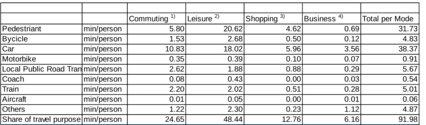
Car transportation usually serves various purposes. In Table 3-1 the use of a passenger car by an aver-age Swiss traveller allocated to four commonly distinguished travel purposes is summarised. In addi-tion to car use, the travel time expenditures for various addiaddi-tional, frequently used transport modes are illustrated. The figures represent the daily travel time of an average Swiss traveller with various means of transportation with respect to four different travel purposes.

Table 3-1: Modal Split with respect to time for an average Swiss traveller (Spielmann et al. 2006)

Commuting 1) _Leisure2) _Shopping3) _Business4) _{Total per Mode}

Pedestriant min/person 5.80 20.62 4.62 0.69 31.73

Bycicle min/person 1.53 2.68 0.50 0.12 4.83

Car min/person 10.83 18.02 5.96 3.56 38.37

Motorbike min/person 0.35 0.39 0.10 0.07 0.91

Local Public Road Tran min/person 2.62 1.88 0.88 0.29 5.67

Coach min/person 0.08 0.43 0.00 0.03 0.54

Train min/person 2.20 2.02 0.51 0.28 5.01

Aircraft min/person 0.01 0.05 0.00 0.01 0.06

Others min/person 1.22 2.30 0.23 1.12 4.87

Share of travel purpose min/person 24.65 48.44 12.76 6.16 91.98

1: Commuting mobility has been derived by aggregating the original categories available from (ARE & SFSO 2000) and includes the following original categories: working trips (100%), education trips (100%) and escort and service trips (25%)

2: Leisure mobility includes leisure trips (100%) and escort and service trips (25%) 3: Shopping mobility includes shopping trips (100%) and escort and service trips (25%)

4: Business mobility includes business activities (100%), travelling on company business (100%) and escort and service trips (25%)

In terms of kilometric performance, an average of 37.3 kilometres travelled by Swiss citizens per day in 2005 is reported in BfS (2007). In Table 3-2, the shares of various used means of transport are shown.

(23)

Table 3-2: Transport means choice (Proportion of average daily distance, 2005). Figure taken from BfS (2007).

For Europe in Eurostat (2007) an average of 36 kilometres travelled by EU citizens per day in 2004 is reported, including daily commute and other activities necessitating transport such as tourism. Car transport accounting for nearly three quarters of this total (26.5 km). This mode was followed, a long way behind, by buses/coaches and air transport (3 km each), railways (2 km), powered-two wheelers (1 km), trams and metros (0.5 km) and sea (0.3 km). It should be noted that non-motorised forms of transport are excluded from the analysis.

3.2 Freight Transport Services

Road freight performance reported by EU and Norwegian hauliers (excluding hauliers from Greece and Malta) in 2004 was 1 677 billion tonne-kilometres (Eurostat 2006). As illustrated in Figure 3-1 More than one third of this total was formed by goods of the NST/R classification 20-24, comprising vehicles and transport equipment, machinery, apparatus, engines, whether or not assembled, and parts thereof, manufactures of metal, glass, glassware, ceramic products, leather, textiles, clothing, other manufactured articles, miscellaneous articles. Miscellaneous articles’ and ‘Leather, textile, clothing, other manufactured articles’ comprised 16% and 10% respectively of total tonne-kilometres. Crude and manufactured minerals, building materials was the second largest group of goods with 17%, closely followed by foodstuffs and animal fodder with 16%.

Figure 3-1: Total transport by type of goods, 2004 - % in tkm. Figure taken from Eurostat (2006)

As illustrated in Figure 3-2 the picture is however very different when considering tonnes carried, al-most half of the 15.2 billion tonnes carried by road by hauliers registered in the EU25 and Norway in 2004 was Crude and manufactured minerals and building materials. (Eurostat 2006)

(24)

Figure 3-2: Total transport by type of goods, 2004 – % in tonnes. Figure taken from Eurostat (2006)

4.5% of the goods transported in 2004 were dangerous goods. Over half of these 75 billion tonne-kilometres were in the category ‘Flammable liquids’ (57%). Only two other categories recorded more than 10%: ‘Gases, compressed, liquefied, dissolved under pressure’ was second with 14%, followed by ‘Corrosives’ at 11%.

(25)

4 System

Characterisation

4.1 Scope of the Project

In ecoinvent 2000 life cycle inventories for four means of goods and passenger transport are modelled:

• Road transportation

• Rail transportation

• Air transportation

• Water transportion

Each mode of transport is further separated into sub-groups, referred to as transport services, using several criteria such as geographical operation (e.g., rail transport), vehicle size (e.g., road transport) and transported goods (e.g., water transport).

4.2 Functional

Unit

In order to relate transport modules to life cycles of other products and services the environmental in-terventions are related to the reference unit of one tonne kilometre [tkm]. A tonne kilometre is defined as: “unit of measure of goods transport, which represents the transport of one tonne of goods by a cer-tain means of transportation over one kilometre”. For passenger transportation, the reference unit of one passenger kilometre [pkm] has been applied.

4.3 Model Structure

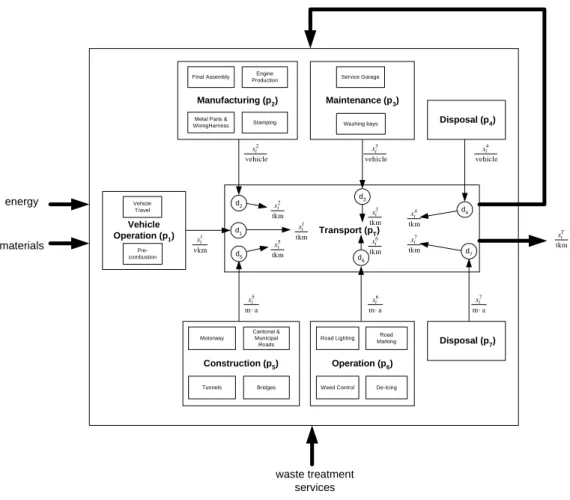
Each mode of transport is further separated into sub-groups, referred to as transport services. In Figure 4-1, the general model structure is illustrated using the example of road freight transport. The

mod-elled transport components (pi, i=1…7) are linked in a unit process (pT) referred to in the database as

“transport, transport service” (e.g. transport, lorry 16t). In order to link various transport components

to the reference flow of one tonne kilometre (tkm), so-called demand factors dj are determined.

Cumu-lative LCI results for a transport service, per tkm are calculated as follows:

∑

= ⋅ = n j j j j i T i d ) p ( r x x 1 (1)

where n denotes the number of transport components and ( j)

j

i rp

x indicate the cumulative

(26)

Disposal (p4) Disposal (p7) d2 vkm 1 i x vehicle 2 i x vehicle 3 i x Vehicle Operation (p1) Vehicle Travel Pre-combustion a m 5 ⋅ i x d5 a m 6 ⋅ i x d₆ a m 7 ⋅ i x d7 d1 tkm 2 i x d₃ d₄ Transport (p_T) Construction (p5) Motorway Bridges Tunnels Cantonal & Municipal Roads Operation (p6) Road Lighting De-Icing Weed Control Road Marking Manufacturing (p₂) Final Assembly Stamping Metal Parts & WiringHarness Engine Production Maintenance (p₃) Service Garage Washing bays vehicle 4 i x tkm 1 i x tkm 5 i x tkm 4 i x tkm 7 i x tkm 3 i x tkm 6 i x energy materials waste treatment services tkm T i x

Figure 4-1: Principle model structure and transport components and their interrelationship (Spielmann & Scholz 2005)

In this report, transport components are frequently organised in three groups, as follows:

Vehicle Operation: The first component contains all processes that are directly connected with the operation of the vehicles. In this project the focus is on fuel consumption and airborne emissions. Par-ticular attention has been paid to the issue of particulate emissions. The only interface to other ecoin-vent modules are fuel supply, or in case of rail systems, electricity supply. For vehicle operation of rail- and road transportation we further distinguish average Swiss conditions and European conditions. The reference unit for operation is tonne kilometre [tkm] and in case of road transport vehicle kilome-tre [vkm]

Vehicle Fleet: Vehicle fleet comprises three components that are connected with the vehicle life cycle (excluding the operation) such as vehicle and part manufacture, vehicle maintenance and support as well as disposal of motor vehicles and parts. The data of the referring modules represent mainly Euro-pean conditions. The reference unit for unit processes of this transport component is one vehicle [unit].

Transport Infrastructure: Transport infrastructure comprises three components addressing construc-tion, operation and maintenance and disposal of the transport infrastructure. In contrast to the previous component the generated data predominately describes Swiss conditions. Land use data is recorded in the unit process “operation and maintenance”. Due to the fact that various elements of infrastructure are characterised by a different life span all data is calculated for one year. Thus the reference unit

(27)

4.4 Data Requirements and Assumptions

4.4.1 Temporal

Scope

The figures for vehicle operation generally refer to the situation in 2000. For the infrastructure data however, such data was often not available. Thus, older data had to be employed, representing a situa-tion somewhere in the last decade. For the new and updates road transport datasets, if not stated ex-plicitly in the name of the datasets, the reference year is 2005.

A crucial assumption that has been made in this study, is to model all material or service inputs, which are situated in the past, with the current (2000) production and service standards. For instance, con-crete, which has been used in the construction of airports in 1980, is represented by a state of the art production in 2000.

The description of infrastructure processes is generally limited to the amount of used bulk materials (such as steel, aluminium, copper, wood, rubber and synthetics) and energy consumption for manufac-turing or construction activities. Furthermore, material and energy consumption due to maintenance activities and disposal of bulk materials are taken into account. For vehicles the disposal of bulk mate-rials is also considered. For transport infrastructure, the disposal has neglected in most cases. Also, ad-ditional material and energy expenditures, e.g., for the production of machinery, have been neglected. The allocation of infrastructure processes to the actual transport performance [tkm] is complex. In this study we use a static approach. First, the material and energy expenditures for the entire transport in-frastructure network are determined and a certain life span for the inin-frastructure (or parts of the infra-structure) is assumed. Thus, an annual average consumption can be calculated. Furthermore, in order to link the infrastructure processes to the functional unit of one tonne kilometre [tkm] we assume that current (2000) performance figures also represent an average for the past and future situation.

4.4.2 Geographical

Scope

The transport modules represent the Swiss conditions and/or European conditions. For rail and road transport infrastructure, data has only been collected for Switzerland and is assumed to represent European conditions as well.

Transport infrastructure is not solely used for goods transportation. Thus, allocation between passen-ger and goods transportation is unavoidable. In general, we use the gross tonne kilometre performance as allocation factor for infrastructure construction and maintenance. For infrastructure operation and maintenance, including land use, we employ the vehicle kilometric performance as allocation rule.

(28)

5 Life Cycle Inventories for Road Transportation

5.1 Classification of Emission Factors for Vehicle Operation

Vehicle operation contains all processes directly connected with the operation of the vehicles, i.e., tail pipe (exhaust) emissions and emissions due to tyre abrasion. In the context of ecoinvent, fuel con-sumption is also included.

According to the source of emissions and the approach employed, emissions determined in this report can be distinguished in into six groups.

• Group 1: Airborne exhaust emissions dependent on fuel consumption and composition

(qual-ity). The basis for the calculation of emission factors are so-called “emissions indices” (EI). The EI is defined as the mass of substance in grams per kilogram of fuel burned.

• Group 2: Airborne regulated exhaust pollutants

• Group 3: Hydrocarbon exhaust emission profiles, which are derived as a fraction of total

NMHC emissions.

• Group 4: Other airborne exhaust emissions

• Group 5: Airborne non-exhaust abrasion particle emissions including fractions of heavy

met-als

• Group 6: Heavy metal emissions to soil and water due to tyre abrasion

In Table 5-1 and

(29)

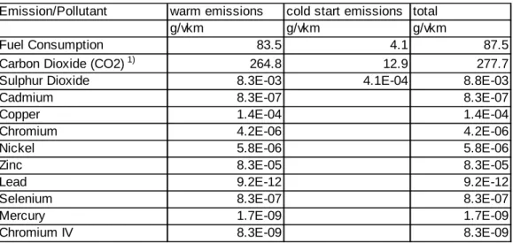
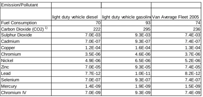
Table 5-1: Emissions included in each emission group (part 1)

Group Emission/Pollutant Remarks

Carbon Dioxide (CO2) Warm emissions. For passenger cars and vans, cold start emis-sions are accounted for, too. Value is directly derived from the fuel consumption, taken into account carbon fixed in CO emissions. Sulphur Dioxide Warm emissions. For passenger cars and vans, cold start

emis-sions are accounted for, too. Cadmium Trace Elements in fuel. Copper Trace Elements in fuel. Chromium Trace Elements in fuel. Nickel Trace Elements in fuel. Selenium Trace Elements in fuel. Zinc Trace Elements in fuel. Lead Trace Elements in fuel. Mercury Trace Elements in fuel.

1

Chromium IV assumption: 0.2% of the emitted Cr is emitted as Cr(IV)

Carbon Monoxide Warm emissions. For passenger cars and vans, cold start emis-sions as well as evaporation are accounted for, too.

Nitrogen Oxides (NOx) Including NO and NO2. Given as NO2 equivalent. Warm emissions. For cars and vans, cold start emissions are accounted for, too. Particulate Matter (PM) Value corresponds to PM2.5. Coarse exhaust PM (PM10) is

consid-ered negligible, hence: PM2.5=PM10. Warm exhaust emissions. For cars and vans, cold start emissions are accounted for, too.

2

Hydrocarbons (HC) Total hydrocarbon emissions. Warm emissions. For cars and vans, cold start emissions as well as evaporation are accounted for, too. Methane (CH4) Warm emissions. For passenger cars and vans, cold start

emis-sions are accounted for, too.

Toulene (C7H8) Warm emissions. For cars and vans, cold start emissions as well as evaporation (for petrol engines) are accounted for, too.

Benzene (C6H6) Warm emissions. For cars and vans, cold start emissions as well as evaporation (for petrol engines) are accounted for, too.

m,p,o Xylene (C8H10) Warm emissions. For cars and vans, cold start emissions as well as evaporation (for petrol engines) are accounted for, too.

Formaldehyde (CH2O) Exhaust emissions, no further specification available. Acetaldehyde

(CH3CHO)

Exhaust emissions, no further specification available.

3

NMHC Total non methane hydrocarbon emissions. According to ecoinvent data requirements the final inventory data, excludes the fractions of toluene, benzene, xylene, formaldehyde and acetaldehyde.

Ammonia (NH3) Warm exhaust emissions. Nitrous Oxide (N2O) Warm exhaust emissions.

4

(30)

Table 5-2: Emissions included in each emission group (part 2)

TSP-PM10 Including tyre wear, break wear and road surface abrasion emis-sions

PM10-PM2.5 Including tyre wear, break wear and road surface abrasion emis-sions

PM2.5 Including tyre wear, break wear and road surface abrasion emis-sions

Zinc Including tyre wear and break wear abrasion emissions

Cooper Including tyre wear and break wear abrasion emissions

Cadmium Including tyre wear and break wear abrasion emissions

Chrome Including tyre wear and break wear abrasion emissions

Nickel Including tyre wear and break wear abrasion emissions

Lead Including tyre wear and break wear abrasion emissions

5

Benzo(a)pyrene Including tyre wear and break wear abrasion emissions

Zinc, ion Emissions to water based on tyre abrasion

Cooper, ion Emissions to water based on tyre abrasion Cadmium, ion Emissions to water based on tyre abrasion Chromium, ion Emissions to water based on tyre abrasion Nickel, ion Emissions to water based on tyre abrasion Lead Emissions to water based on tyre abrasion

Zinc Emissions to soil based on tyre abrasion

Cooper Emissions to soil based on tyre abrasion Cadmium Emissions to soil based on tyre abrasion Chrome Emissions to soil based on tyre abrasion Nickel Emissions to soil based on tyre abrasion

6

Lead Emissions to soil based on tyre abrasion

5.2 General Assumptions for Emission Factors

5.2.1 Group 1: Emissions Indices

Carbon dioxide and sulphur dioxide emissions are directly derived from the fuel consumption and car-bon content or sulphur content of the used fuel, respectively.

For the determination of CO2-emissions we employ a conversion factor of 3.172 kgCO2/kgFuel

(assum-ing a C-content of 86.5 w.% in both, diesel and petrol fuels (Jungbluth 2003)). The final value for the

life cycle inventories is then derived by subtracting the carbon fixed in CO-emissions. For SO2

-emissions we assume a sulphur content of 50mgS/kgfuel , i.e. 100mgSO2/kgfuel (ecoinvent fuel

proper-ties(Jungbluth 2003)). It should be noted, that in Keller (2004) different conversion factor are

pre-sented: 0.02 gSO2/kgdiesel (0.001 w.%) and 0.016 gSO2/kgpetrol (0.0008 w.%), for diesel powered cars and

petrol powered cars, respectively.

Emission indices for heavy metal emissions due to trace elements in the fuels are presented in Table 5-3.

(31)

Table 5-3: Emission indices for heavy metal emissions Petrol Diesel mg/kg mg/kg Cadmium 1) Cd 0.01 0.01 Copper 1) Cu 1.7 1.7 Chromium 1) Cr 0.05 0.05 Nickel 1) Ni 0.07 0.07 Selenium 1) Se 0.01 0.01 Zinc 1) Zn 1 1

Lead 2) Pb 2.E-03 1.10E-07

Mercury 2) Hg 7.E-05 2.E-05

Chromium IV 3) Cr(VI) 1.0E-04 1.0E-04

1: taken from EMEP/CORINAIR (2006) 2: derived from Jungbluth (2003)

3: underlying assumption: 0.2% of the emitted Cr is emitted as Cr(IV)

5.2.2 Group 2: Regulated Exhaust Pollutants

For the determination of combustion process-specific EURO-regulated exhaust emissions (HC, CO,

NOx and particles) Swiss figures are based on measurements carried out on chassis dynamometers

us-ing realistic drivus-ing patterns for Switzerland. These figures are different from the type approval cycles (de Haan & Keller 2004; de Haan & Keller 2004; Keller & Zbinden 2004). The employed figures in-clude cold start emissions and for petrol vehicles emissions from vaporisation. In addition ageing ef-fects of the catalytic converter are included. In order to convert cold start emissions per start and evaporation per stop to the reference unit of one vehicle kilometre, the values presented in Table 5-5 are used.

European data is derived from (TREMOVE 2007), which again is generated from various runs with COPERT (2006). The underlying methodology and major assumptions are presented in (EMEP/CORINAIR 2006).

5.2.3 Group 3: Hydrocarbon exhaust emission profiles

In Table 5-4 hydrocarbon exhaust emission profiles, which are derived as a fraction of total NMHC emissions are presented. Obviously, there are slight differences between the data obtained from EMEP/CORINAIR (2006) and Keller (2004). The latter is assumed to describe more precisely Swiss conditions and thus is applied for all Swiss transport datasets. In addition emission shares of formalde-hyde and acetaldeformalde-hyde available from EMEP/CORINAIR (2006) are applied to Swiss datasets. For the European transport datasets we use the data derived from EMEP/CORINAIR (2006).

Table 5-4: Hydrocarbon exhaust emission profiles, which are derived as a fraction of total NMHC emissions

CorineAir 2)

warm start evaporation PC & LDV HDV warm start evaporation Euro1 & on Toulene C7H8 0.29% 0.29% 0.00% 0.69% 0.01% 8.52% 9.93% 3.00% 10.98%

Benzene C6H6 1.66% 1.14% 0.00% 1.98% 0.07% 11.82% 6.44% 0.80% 5.61%

m,p,o Xylene C8H10 0.78% 0.78% 0.00% 1.38% 0.88% 7.05% 9.36% 1.00% 7.69%

Formaldehyde CH2O n.a. n.a. n.a. 12.00% 8.40% n.a. n.a. n.a. 1.70%

Acetaldehyde CH3CHO n.a. n.a. n.a. 6.47% 4.57% n.a. n.a. n.a. 0.75%

Emission

Diesel Petrol

HBEFA 1) _CorineAir2) _HBEFA1)

1: data derived from Keller (2004)

(32)

Table 5-5: Start/stop performances for the calculation of cold start and evaporation emissions of Swiss passenger cars and vans.

year 2005 2010 2005 2010

starts per year Mio starts/a 3762 3892 199 205

kilometric performance Mio vkm/a 53689 56537 4343 4635

starts per vkm starts/vkm 0.070 0.069 0.046 0.044

trip length vkm/start 14.27 14.53 21.82 22.61

PC Van

5.2.4 Group 4: Other exhaust emissions

Nitrous Oxides (N

2

O) and Ammonia (NH

3

)

Data for N2O and NH3 is directly available for Switzerland from Keller (2004). For Europe,

TREMOVE (2007), merely delivers N2O emissions. Thus, as a first approximation NH3 values from

Keller (2004) are employed for Europe, too.

PAHs

Polycyclic Aromatic Hydrocarbons (PAHs) emissions of diesel cars (0.7E-6 g/vkm for a direct injec-tion concept) and petrol cars (0.4E-06g/vkm) are taken from EMEP/CORINAIR (2005). Whilst the uncertainty of the emission factor for diesel cars is reported to be low (0.3-1.0E-9 kg/vkm), the aver-age emission factor presented for petrol concepts is fairly high (0.001-8.8E-09 kg/vkm). Thus we ad-justed the uncertainty factor for the latter concept. For heavy duty vehicles we apply the best estimate 1.0E-06 g/vkm. The uncertainty range is assumed to be 0.02E-06 – 6.2E-06 g/vkm)

5.2.5 Group 5: Non-exhaust abrasion particle emissions including fractions

of heavy metals

The emission factors for non exhaust abrasion particle emissions are based on assumptions and data presented in EMEP/CORINAIR (2003) Three categories of non-exhaust emissions are distinguished: tyre wear, break wear and road abrasion. In following parts, some basic information is given and the emission factors applied in ecoinvent v2.0 are presented. It should be noted, that the definition of par-ticles in EMEP/CORINAIR (2003) differs from ecoinvent particle size classifications. Thus, the data has been adjusted to match ecoinvent methodology. Particle emissions with a diameter up to 100 µm may generally be considered as airborne emissions (TSP). Practically, particles larger than 100 µm have residence times of only seconds to minutes (depending on turbulence), and are generally consid-ered as dustfall.

Tyre Wear Emitted Particles

Tyre wear material is emitted across the whole size range for airborne particles. Camatini (2001) col-lected debris from the road of a tyre proving ground. They found tyre debris agglomerated to particle sizes up to a few hundred micrometers. As stated above, such particles are not airborne and are of lim-ited interest to air pollution, but they contribute the largest fraction by weight of total tyre wear. In ecoinvent, the heavy metal content of these emissions is accounted for as emission to water and soil (see emission group 7). In Table 5-6 the size distribution of tyre wear emitted particles is summarised. In Table 5-7 the resulting emission factors for tyre wear emitted particles according to ecoinvent clas-sification are presented.

Table 5-6: Size distribution of tyre wear emitted particles

Particle size class Mass fraction of TSP

TSP 1

PM10 0.6

(33)

Table 5-7: Emission factors for tyre wear emitted particles according to ecoinvent classification TSP-PM10 PM10-PM2.5 PM2.5 TSP g/vkm g/vkm g/vkm g/vkm Passenger Cars 0.0043 0.0037 0.0027 0.0107 Vans 0.0068 0.0059 0.0043 0.0169 Lorry 0.0180 0.0157 0.0113 0.0450

Brake Wear Emitted Particles

Brakes are used to decelerate a vehicle. There are two main brake system configurations in current use: disc brakes, in which flat brake pads are forced against a rotating metal disc, and drum brakes, in which curved pads are forced against the inner surface of a rotating cylinder (EMEP/CORINAIR 2003). Disc brakes tend to be used in smaller vehicles (passenger cars and motorcycles) and in the front wheels of light-duty trucks, whereas drum brakes tend to be used in heavier vehicles. Linings generally consist of four main components: binders, fibres, fillers, and friction. Various modified phe-nol-formaldehyde resins are used as the binders. Fibres can be classified as metallic, mineral, ceramic, or aramide, and include steel, copper, brass, potassium titanate, glass, asbestos, organic material, and Kevlar. Fillers tend to be low-cost materials such as barium and antimony sulphate, kaolinite clays, magnesium and chromium oxides, and metal powders. Friction modifiers can be of inorganic, organic, or metallic composition. Graphite is a major modifier used to influence friction, but other modifiers include cashew dust, ground rubber, and carbon black. In the past, brake pads included asbestos fibres, though these have now been totally removed from the European fleet.

In Table 5-8 the size distribution of brake wear emitted particles is summarised. In Table 5-9 the re-sulting emission factors for brake wear emitted particles according to ecoinvent classification is pre-sented.

Table 5-8: Size distribution of brake wear emitted particles

TSP 1

PM10 0.98

PM2.5 0.42

Table 5-9: Emission factors for brake wear emitted particles according to ecoinvent classification

TSP-PM10 PM10-PM2.5 PM2.5 TSP

g/vkm g/vkm g/vkm g/vkm

Passenger Cars 0.0002 0.0043 0.0031 0.0075

Vans 0.0002 0.0067 0.0048 0.0117

Lorry 0.0006 0.0182 0.0132 0.0320

Particle Emissions from Road Surface

The wear rate of asphalt, at least in terms of airborne wear particles, is even more difficult to quantify than tyre and brake wear, partly because the complex chemical composition of bitumen, and partly be-cause primary wear particles mix with road dust and suspended material. Therefore, the presented wear rates and particle emission rates for road surfaces are highly uncertain.

In Table 5-10 the size distribution of road surface emitted particles is summarised. In Table 5-11 the resulting emission factors for road surface emitted particles according to ecoinvent classification is presented.

(34)

Table 5-10: Size distribution of road surface emitted particles

TSP 1

PM10 0.5

PM2.5 0.27

Table 5-11: Emission factors for road surface emitted particles according to ecoinvent classification

TSP-PM10 PM10-PM2.5 PM2.5 TSP

Passenger Cars 0.0075 0.0055 0.0020 0.0150

Vans 0.0075 0.0055 0.0020 0.0150

Lorry 0.0380 0.0277 0.0103 0.0760

Total Non-Exhaust Particle Emissions

In Table 5-12 the total non exhaust particle emissions are summarised.

Table 5-12: Emission factors for road surface emitted particles according to ecoinvent classification

Particle size class Passenger Car Van Lorry

TSP-PM10 g/vkm 0.012 0.014 0.057

PM10-PM2.5 g/vkm 0.013 0.018 0.062

PM2.5 g/vkm 0.008 0.011 0.035

TSP g/vkm 0.033 0.044 0.153

Uncertainties

The emission factors provided in this section are based on EMEP/CORINAIR (2003). The data is re-ported to have been developed on the basis of information collected by literature review, and on wear rate experiments.

The emission factor values proposed in this Chapter have also been crosschecked with inventory ac-tivities and as a rule of thumb, an uncertainty in the order of ±50% is expected for tyre wear and brake wear. For road surface emissions uncertainties are expected to be significantly higher.

Heavy Metal Species Profile

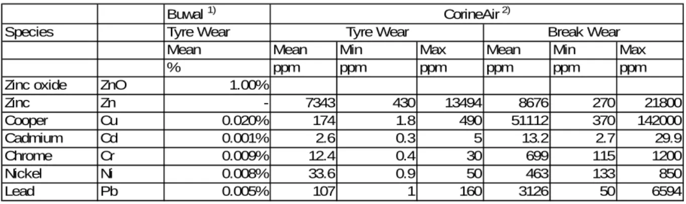
Table 13 provides the speciation of tyre and brake wear into different elements. Data is available from BUWAL (2000) and (EMEP/CORINAIR 2003). For the latter, which is used for ecoinvent v2.0, sev-eral sources have been used to provide this speciation and for this reason, a mean value and the mini-mum and maximini-mum values are shown. In several instances a large range is reported. This is obviously due to the variety of materials and sources used to manufacture tyre tread and brake linings, and a lar-ger sample of materials needs to be studied. At present, due to the absence of such information the "mean" value is a non-weighted average of values given in different reports. For the latter, The latter is used in this research.

(35)

Table 5-13: Element specification of tyre and brake wear. Data used in ecoinvent is EMEP/CORINAIR (2003)

Buwal 1)

Species Tyre Wear

Mean Mean Min Max Mean Min Max

% ppm ppm ppm ppm ppm ppm

Zinc oxide ZnO 1.00%

Zinc Zn - 7343 430 13494 8676 270 21800 Cooper Cu 0.020% 174 1.8 490 51112 370 142000 Cadmium Cd 0.001% 2.6 0.3 5 13.2 2.7 29.9 Chrome Cr 0.009% 12.4 0.4 30 699 115 1200 Nickel Ni 0.008% 33.6 0.9 50 463 133 850 Lead Pb 0.005% 107 1 160 3126 50 6594 CorineAir 2)

Tyre Wear Break Wear

1: BUWAL (2000)

2: data available from EMEP/CORINAIR (2003)

5.2.6 Group 7: Emissions to soil and water

As stated above only a fraction of the tyre abrasion is emitted to air. The remaining fraction is assumed to be emitted to soil and water close to roads or is fixed in the roadway. As far as heavy metals fixed in the roadway are concerned, we assume that they finally will enter the natural environment due to road cleaning activities or rainfall. Since no further information on the share of emissions to soil and water (e.g. canalisation) is readily available we assume that 50% of the abrasion, which is not emitted to air, is emitted to soil and another 50% is emitted to water. In Table 5-14 the resulting abrasions fig-ures and underlying assumptions are summarised.

Table 5-14: Non-airborne tyre wear losses

passenger car van lorry 16t lorry 28t lorry 40t

Performance vehicle vkm/v 150000 235000 540000 540000 540000

a 3 3 - -

-km 45000 45000 75000 75000 75000

Weight tyre kg 8 8 47.5 47.5 47.5

Losses % 15.00% 15.00% 20.00% 20.00% 20.00%

Abrasion per tyre kg 1.2 1.2 9.5 9.5 9.5

Number of tyres per vehicle 4 4 6 12 14

Number of tyres per vehicle lifet time 13.33 20.89 43.20 86.40 100.80

Total abrasion g/vkm 0.11 0.11 0.76 1.52 1.77

Airborne emissions g/vkm 0.0332 0.0436 0.1530 0.1530 0.1530

Remaining Losses g/vkm 0.07 0.06 0.61 1.37 1.62

Life span tyre set

5.3 Life Cycle Inventories for the Operation of Swiss Passenger

Cars (Average Fleet)

Since 1996 the European emission limits for newly registered road vehicles (Euro standards) also be-came effective in Switzerland. Euro3 and Euro4 be-came into force in January 2001 and January 2006, respectively. In Table 5-15 the technology composition of the Swiss average fleet for the years 2005 and 2010 are presented, differentiated with respect to engine type.