2018
Selection and assessment of bivariate Markov
random field models
Yeon-Jung Seo
Iowa State University
Follow this and additional works at:
https://lib.dr.iastate.edu/etd
Part of the
Statistics and Probability Commons
This Dissertation is brought to you for free and open access by the Iowa State University Capstones, Theses and Dissertations at Iowa State University Digital Repository. It has been accepted for inclusion in Graduate Theses and Dissertations by an authorized administrator of Iowa State University Digital Repository. For more information, please [email protected].
Recommended Citation
Seo, Yeon-Jung, "Selection and assessment of bivariate Markov random field models" (2018).Graduate Theses and Dissertations. 17311.
by
Yeon-jung Seo
A dissertation submitted to the graduate faculty in partial fulfillment of the requirements for the degree of
DOCTOR OF PHILOSOPHY
Major: Statistics
Program of Study Committee: Petruta C. Caragea, Co-major Professor
Mark S. Kaiser, Co-major Professor Kris De Brabanter
William A. Gallus Jarad Niemi
The student author, whose presentation of the scholarship herein was approved by the program of study committee, is solely responsible for the content of this dissertation. The Graduate College will ensure this dissertation is globally accessible and will not permit alterations after a degree is
conferred.
Iowa State University Ames, Iowa
2018
DEDICATION
I would like to dedicate this dissertation to my parents and my dear friends, Jerold Mathews and his wife, Eleanor Mathews, for all of their love and a constant source of support and
TABLE OF CONTENTS Page LIST OF TABLES . . . vi LIST OF FIGURES . . . x ACKNOWLEDGMENTS . . . xiv ABSTRACT . . . xv CHAPTER 1. INTRODUCTION . . . 1
1.1 General Introduction and Outline . . . 1
1.2 Literature Review: Multivariate Gaussian MRF Models . . . 2
CHAPTER 2. ALTERNATIVE SPATIAL DEPENDENCE STRUCTURES IN BIVARIATE GAUSSIAN MARKOV RANDOM FIELD MODELS . . . 10
2.1 Introduction . . . 10
2.2 Preliminaries . . . 11
2.2.1 Univariate Gaussian MRF . . . 11
2.2.2 Multivariate Gaussian MRF . . . 13
2.3 Formulation of Gaussian MRF Models for Bivariate Observations . . . 15
2.3.1 Two-independent MRFs model . . . 15
2.3.2 Two-variable MRF . . . 16
2.3.3 Bivariate MRF . . . 17
2.3.4 Extended two-variable MRF . . . 19
2.3.5 Neighborhood structures . . . 21
2.4 Modeled and Implied Dependence Structures . . . 21
2.4.2 Properties of the two-variable MRF . . . 23
2.4.3 Properties of the bivariate MRF model . . . 24
2.4.4 Properties of the extended two-variable MRF model . . . 26
2.4.5 Conditional correlation structures . . . 28
2.5 Parameter Spaces for the Bivariate and Extended Two-variable MRF Models . . . . 28
2.5.1 Parameter space for the bivariate MRF . . . 30
2.5.2 Parameter space for the extended two-variable MRF . . . 30
2.6 Comparison of Conditional Dependencies and Model “Matching” . . . 33
2.7 Summary and Concluding Remarks . . . 35
CHAPTER 3. ASSESSMENT OF BIVARIATE GAUSSIAN MARKOV RANDOM FIELD MODELS BASED ON SPATIAL BLOCKWISE EMPIRICAL LIKELIHOOD (SBEL) . . 42
3.1 Introduction . . . 42
3.2 Univariate Gaussian MRF Model . . . 45
3.3 Bivariate Gaussian MRF Models . . . 46
3.3.1 Two-independent MRFs model . . . 48
3.3.2 Two-variable MRF . . . 49
3.3.3 Bivariate MRF . . . 50
3.3.4 Extended two-variable MRF . . . 52
3.3.5 Conditional dependence structures of the four models . . . 53
3.4 Constructing an SBEL Procedure for Model Assessment . . . 56
3.4.1 SBEL construction for spatial lattice data . . . 56
3.4.2 Spatial estimating functions for bivariate models . . . 61
3.5 Simulation Study: Assessments of Bivariate Gaussian MRF Models . . . 64
3.5.1 Assessment of inter-variable independence structure under two-independent MRFs . . . 65 3.5.2 Assessment ofcross-variable independence structure under two-variable MRF 66
3.5.3 Assessment of homogeneouscross-variableandwithin-variable spatial depen-dence structures under bivariate MRF . . . 67 3.6 Verifying conditional dependence structure in modeling daily average temperatures
and dew points in Iowa . . . 71 3.7 Concluding Remarks . . . 77 BIBLIOGRAPHY . . . 81 APPENDIX A. ESTIMATING FUNCTIONS USED FOR BIVARIATE MODEL
ASSESS-MENTS, SECTION3.4.2 . . . 84 APPENDIX B. SUMMARY OF THE SBEL SIMULATION RESULTS IN SECTION3.5 . . 87
LIST OF TABLES
Page
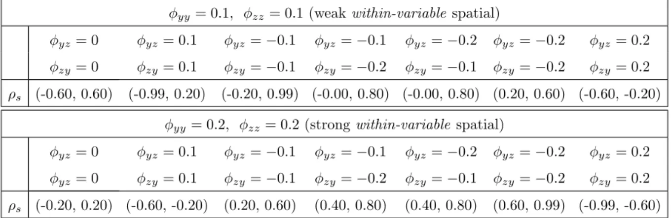
Table 2.1 Lower and upper bounds of parameter spaces for spatial dependence, η, in the bivariate MRF model, with four-nearest neighbors, as a function of lattice sizek×k. . . 30 Table 2.2 Valid parameter space for ρs, for fixed values of (φyy, φzz, φyz, φzy) with
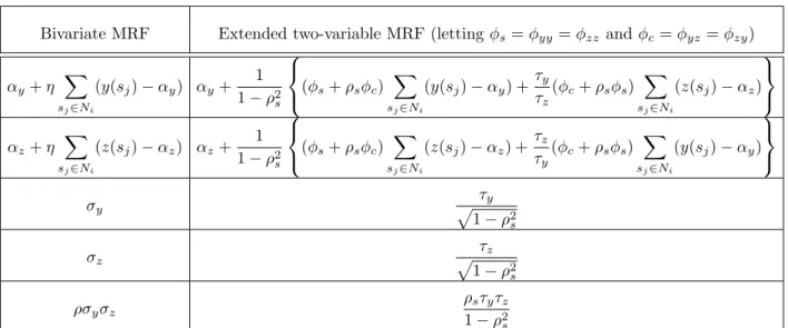
four-nearest neighborhood structure (30×30 lattice), in the extended two-variable MRF model. . . 32 Table 2.3 Side-by-side comparison of bivariate full conditionals for the bivariate and
extended two-variable MRF specifications. . . 35
Table 3.1 Spatial data-generating models considered in fitting the null H0 : The mo-ment condition holds for some parameterθ0 under two-independent MRFs. For all models in the table, we used αy = αz = 0, τy = τz = 1, and σy = σz = 1. When generating data from the bivariate MRF model, five different values of correlation coefficient,ρ= 0.01,0.1,0.2,0.4,0.8, were cho-sen for each (4- or 8-nearest) neighborhood structure. See Figure3.6. (The result fromρ= 0.8 is not shown.) . . . 68 Table 3.2 Spatial data-generating models considered in fitting the null H0 : The
mo-ment condition holds for some parameter θ0 under two-variable MRF. For all models in the table, we usedαy =αz = 0,τy =τz = 1, and σy =σz= 1. When generating data from the bivariate MRF model, five different values of correlation coefficient, ρ= 0.01,0.1,0.2,0.4,0.8, were chosen for each (4-or 8-nearest) neighb(4-orhood structure. See Figure3.7. . . 68
Table 3.3 Spatial data-generating models considered in fitting the null H0 : The mo-ment condition holds for some parameter θ0 under bivariate MRF. For all models in the table, we used αy = αz = 0, τy = τz = 1, or σy = σz = 1. When generating data from the extended two-variable MRF model, the fol-lowing four scenarios are considered in the neighborhood structure (e.g., both equal spatial and equal cross dependencies, etc.): (i) φyy = φzz and
φyz =φzy, (ii) φyy =φzz and φyz 6=φzy, (iii) φyy 6=φzz andφyz =φzy, and
(iv)φyy6=φzz andφyz 6=φzy, for a choice of eitherρs= 0.2 orρs= 0.6, with 4-nearest spatial neighbors. For bivariate MRF, the values of ρ = 0.2,0.6 are used in the simulations assuming the 4-nearest neighborhood structure. See Figure3.8. . . 69
Table B.1 Actual size of SBEL tests for assessing the null (two-independent MRFs model) at nominal levels of 0.01,0.05, and 0.10 when the data-generating models belong to the null (see Table3.1). See also Figure 3.6. . . 87 Table B.2 Mean and median parameter estimates for θ = (αy, αz, ηy, ηz, τy, τz)0 from
SBEL in fitting the null (two-independent MRFs model assessing inter-variableindependence structure) and from maximum pseudo-likelihood (MPL). See Figure3.6. Data generation occurs under each of the four cases of the null (see Table 3.1), with a block scaling of b= 1.5n1/5 for a lattice size of 30×30. . . 88 Table B.3 Actual size of SBEL tests for assessing the null (two-variable MRF model)
at nominal levels of 0.01,0.05, and 0.10 when the data-generating models belong to the null (see Table3.2). See also Figure 3.7. . . 89
Table B.4 Mean and median parameter estimates for θ = (αy, αz, ηy, ηz, κy, τy, τz)0
from SBEL in fitting the null (two-variable MRF model assessing cross-variable independence structure) and from maximum pseudo-likelihood (MPL). See Figure3.7. Data generation occurs under each of the four cases of the null (see Table 3.2), with a block scaling of b= 1.5n1/5 for a lattice size of 30×30. . . 90 Table B.5 Actual size of SBEL tests for assessing the null (two-variable MRF model)
at nominal levels of 0.01,0.05, and 0.10 when the data-generating models belong to the null (see Table3.2). See Figure B.1 (b). . . 92 Table B.6 Mean and median parameter estimates for θ = (αy, αz, ηy, ηz, κy, τy, τz)0
from SBEL in fitting the null (two-variable MRF model assessing cross-variable independence structure) and from maximum pseudo-likelihood (MPL). See FigureB.1 (b). Data generation occurs under each of the four cases of the null (see Table 3.2), with a block scaling of b = 3n1/5 for a lattice size of 30×30. . . 92 Table B.7 Actual size of SBEL tests for assessing the null (bivariate MRF model)
at nominal levels of 0.01,0.05, and 0.10 when the data-generating models belong to the null (see Table3.3). See Figure 3.8(a). . . 93 Table B.8 Mean and median parameter estimates for θ = (αy, αz, η, σy, σz, ρ)0 from
SBEL in fitting the null (bivariate MRF model assessing homogeneous cross-variable dependence) and from maximum pseudo-likelihood (MPL). See Fig-ure3.8 (a). Data generation occurs under each of the two cases of the null (see Table3.3), with a block scaling ofb= 1.5n1/5 for a lattice size of 30×30. 93 Table B.9 Actual size of SBEL tests for assessing the null (bivariate MRF model with
equal cross-correlation) at nominal levels of 0.01,0.05, and 0.10 when the data-generating models belong to the extended two-variable MRF (see Table 3.3). See Figure 3.8(b,c,d). . . 94
Table B.10 Median parameter estimates forθ= (αy, αz, η, σy, σz, ρ)0in fitting the null of
the bivariate MRF model to data generated from the extended two-variable MRF models, with regular MPLEs involving each extended two-variable MRF. See Figure3.8 (c). . . 95 Table B.11 Actual size of SBEL tests for assessing the null (bivariate MRF model with
equal spatial-correlation) at nominal levels of 0.01,0.05, and 0.10 when the data-generating models belong to the extended two-variable MRF (see Table 3.3). See Figure 3.9(a,b). . . 96 Table B.12 Actual size of SBEL tests for assessing the null (bivariate MRF model with
both equal cross-correlation and equal spatial-correlation) at nominal lev-els of 0.01,0.05, and 0.10 when the data-generating models belong to the extended two-variable MRF (see Table 3.3). See Figure 3.9 (c,d). . . 97
LIST OF FIGURES
Page
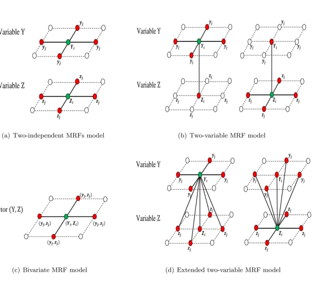
Figure 2.1 Illustration of four MRF specifications with four-nearest (spatial) neighbor-hood structure. The random variables Y(si) and Z(si) are denoted by Yi
and Zi (with green dots), respectively; and for each random variable its
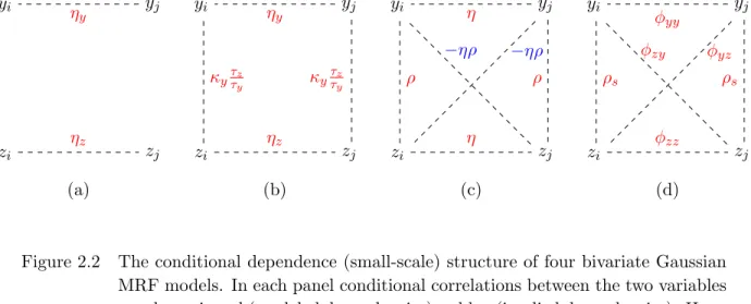
neighbors are indicated by solid lines and red dots. The subscriptj is used to indicate the observations in the neighboring locations (yj orzj). . . 22 Figure 2.2 The conditional dependence (small-scale) structure of four bivariate
Gaus-sian MRF models. In each panel conditional correlations between the two variables are shown in red (modeled dependencies) or blue (implied de-pendencies). Here, (yi, zi) and (yj, zj) denote the vectors of bivariate
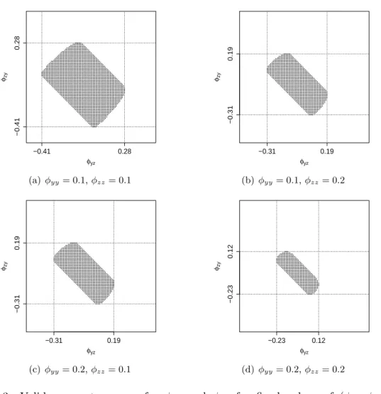
ob-servations from two neighboring sites, si and sj, respectively. Panel (a): two-independent MRFs; Panel (b): two-variable MRF; Panel (c): bivariate MRF; and Panel (d): extended two-variable MRF. . . 29 Figure 2.3 Valid parameter space for φyz and φyz for fixed values of (φyy, φzz) with
ρs= 0.2, given a 30×30 lattice with four-nearest neighborhood structures,
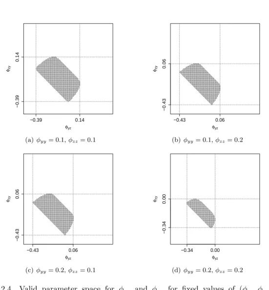
in the extended two-variable MRF model. . . 37 Figure 2.4 Valid parameter space for φyz and φyz for fixed values of (φyy, φzz) with
ρs= 0.6, given a 30×30 lattice with four-nearest neighborhood structures,
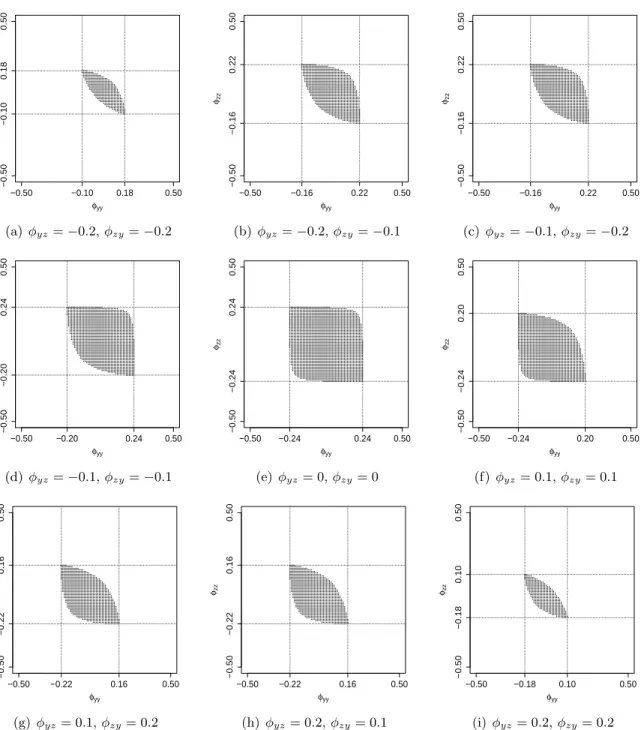
in the extended two-variable MRF model. . . 38 Figure 2.5 Valid parameter space for φyy and φzz for fixed values of (φyz, φzy) when
ρs= 0.2, given a 30×30 lattice with four-nearest neighborhood structures,
Figure 2.6 Valid parameter space for φyy and φzz for fixed values of (φyz, φzy) when ρs= 0.6, given a 30×30 lattice with four-nearest neighborhood structures,
in the extended two-variable MRF model. . . 40 Figure 2.7 Valid parameter space for cross dependence parameter φc = φyz = φyz
for fixed values of (φyy, φzz, ρs), given a 30 ×30 lattice with four-nearest neighborhood structures, in the extended two-variable MRF model. Here, the value of−η×ρ is indicated by “∗” and “−ηρ” for comparison with the bivariate MRF model. . . 41
Figure 3.1 Illustration of four-nearest and eight-nearest neighbors on a regular lattice. . 46 Figure 3.2 Illustration of four MRF specifications with four-nearest (spatial)
neighbor-hood structure. The random variables Y(si) and Z(si) are denoted by Yi
andZi, respectively; and solid lines connect its nearest neighbors. The
sub-scriptj is used to indicate the observations in the neighboring locations (yj
orzj). . . 54 Figure 3.3 The conditional dependence (small-scale) structure of four bivariate
Gaus-sian MRF models. In each panel conditional correlations between the two variables are shown to describe modeled (dashed lines) and induced (dotted lines) dependencies. Here, (yi, zi) and (yj, zj) denote the vectors of bivariate
observations from two neighboring sites, si and sj, respectively. Panel (a): two-independent MRFs, Panel (b): two-variable MRF, Panel (c): bivariate MRF, and Panel (d): extended two-variable MRF. . . 55 Figure 3.4 An example of Dn for 20×20 spatial lattice data (n = 400) with (a) its
sampling sitesSn and (b) data blocks, Bb(ij) within Sn. . . 58
Figure 3.5 Neighboring variables and locations for bivariate data. Left Panel: four-nearest neighborhood structure. Right Panel: eight-four-nearest neighborhood structure. The bold-faced letters denote the variables used to compute the estimating functions in Eq. (3.31). . . 63
Figure 3.6 Power curves for fitting the null model (two-independent MRFs model with dependence parametersηyandηz). Each curve corresponds to the SBEL test
(using b = 1.5n1/5) for fitting the null under each data-generating model, assuming a four-nearest neighborhood structure (Panels (a,b)) and an eight-nearest neighborhood structure (Panels (c,d)). . . 72 Figure 3.7 Power curves for fitting the null model (two-variable MRF model with
de-pendence parameters ηy, ηz, κy, and κz (letting κ≡κy =κz)). Each curve
corresponds to the SBEL test (usingb= 1.5n1/5) for fitting the null under each data-generating model, either two-variable MRF model or bivariate MRF model, assuming a four-nearest neighborhood structure (Panels (a,b)) and an eight-nearest neighborhood structure (Panels (c,d)). . . 73 Figure 3.8 Power curves for fitting the bivariate MRF model, assessing equal
cross-variable dependence structure. Each curve corresponds to the SBEL test (using b = 1.5n1/5) for fitting the null under each data-generating model, either bivariate MRF (Panel (a)) or extended two-variable MRF (Panels (b,c,d)), assuming a four-nearest neighborhood structure. . . 74 Figure 3.9 Power curves for fitting the bivariate MRF model, assessing equal
within-variable spatial dependence structure (Panels (a,b)), and assessing both equalwithin-variable and equalcross-variable dependence structures (Pan-els (c,d)). Each curve corresponds to the SBEL test (using b = 1.5n1/5) for fitting the null (bivariate MRF) under each data-generating model from extended two-variable MRF, assuming a four-nearest neighborhood structure. 75 Figure 3.10 Sampling region (inside the rectangle) used for the SBEL tests. . . 76 Figure 3.11 Two examples of IEM ReAnalysis (IEMRE) gridded datasets, for daily
av-erage temperature (in ◦C) and dew point temperature (in◦C) measured in the sampling region (Figure3.10), on May 11 and July 10 of 2016. . . 79
Figure 3.12 Values of the SBEL test statistics with p-values, for assessments of equality of cross-variable (Panels (a), (c)) and within-variable (Panels (b), (d)) de-pendence structures under the bivariate MRF model. For each test in either Panel (a) or (b), daily average temperatures and dew points observed in the spatial sampling region (Figure3.10) during 2016, are used. . . 80
Figure B.1 Power curves for fitting the null model (two-variable MRF model with de-pendence parameters ηy, ηz, κy, and κz, letting κ ≡ κy = κz). Panel (a)
revisits the plots in Figure 3.7, Panel (a) with b = 1.5n1/5, for a compar-ison. Panel (b) corresponds to the SBEL test using b = 3n1/5, for fitting the null under each data-generating model, either two-variable MRF model or bivariate MRF model, assuming a four-nearest neighborhood structure. The numerical summaries are given in TablesB.5 and B.6. . . 91
ACKNOWLEDGMENTS
I would like to take this opportunity to express my thanks to those who helped me with various aspects of conducting research and the writing of this dissertation. First and foremost, I would like to express my sincere gratitude to my advisors, Drs. Petrut¸a Caragea and Mark Kaiser, for their invaluable guidance, support, and encouragement throughout my research work. Not only have they helped me improve statistical understandings for my research, but also their insightful suggestions and comments have been of great value to me and kept me motivated. I would like to thank my committee members Drs. Kris De Brabanter, William Gallus and Jarad Niemi for their time and patience throughout this process. I would also like to thank the Department of Statistics for providing not only financial support, but also a very friendly environment during my graduate study. I would like to give special thanks to Daryl Herzmann in the department of Agronomy for his time and kind help in finding weather data for my research.
I extend special thanks to Drs. Howard Levine and Marit Nilsen-Hamilton, for their scientific guidance, time, and patience for the continuation of my work in the fields of mathematics and biology. I am grateful for what they have offered me.
I would like to express my warm and sincere thanks to Dr. Jerold Mathews and his wife, Eleanor Mathews, who provided invaluable support, encouragement, friendship and love throughout my long journey in Ames. I am truly grateful for having both of them in my life.
Finally, I would like to express my deepest thanks to my parents, sister, brother, sister-in-law and brother-in-sister-in-law in South Korea for their unconditional love, patience and moral support. Without their support, I could not have made it this far.
ABSTRACT
A multivariate Markov random field (MRF) model can be an appealing approach to an analysis of spatially correlated data, where multiple responses at each location may contain complex depen-dence structures, both across and within the areal units. To develop such a model, a functional form of the conditional distribution (with dependence parameters) for the multiple random vari-ables must be determined. In this work, we study alternative formulations of a bivariate Gaussian MRF which are distinguished by choice of spatial or non-spatial neighborhood structures. We then consider a problem of MRF model assessments to diagnose the adequacy of the model structure (e.g., spatial neighborhood) for observed spatial data. We develop a procedure for assessing a particular dependence structure made in bivariate MRF model formulation, using the method of spatial blockwise empirical likelihood (SBEL). Simulation studies show that the proposed SBEL method provides a way to detect an incorrect assumption of the conditional dependence structure used in bivariate model construction. This procedure is also illustrated with an example of the daily average temperatures and dew points measured in Iowa during 2016.
CHAPTER 1. INTRODUCTION
1.1 General Introduction and Outline
This dissertation focuses on the understanding of underlying statistical properties implied by alternative conditional approaches in the construction of a bivariate Markov random field (MRF) model. It discusses four distinct conditional specifications in modeling for bivariate lattice data, and examines their modeled and implied conditional dependencies to better understand complex statistical dependencies among variables within and across areal units. This study also revisits a method of spatial blockwise empirical likelihood by Nordman (2008) and develops a procedure for assessing a particular dependence structure made in bivariate MRF model formulation, in a manner similar to that suggested for univariate MRFs by Kaiser and Nordman (2012).
Markov random field (MRF) models, proposed by Besag (1974), are commonly used in the analysis of spatial data, particularly when measurements are observed on a lattice. The MRF ap-proach to constructing statistical models is based on the specification of conditional distributions for each location, borrowing information from a collection of spatially close sites, called a neighbor-hood. This work focuses on Gaussian MRF models, where conditional distributions are assumed Gaussian, commonly referred to as conditional autoregressive (CAR) model specifications.
Chapter 2 discusses four alternative conditional dependence structures specified in a bivariate MRF model construction, including the formulations proposed by Mardia (1988) and Sain et al. (2011). These two formulations differ where the former specifies the multivariate full conditional distribution of the random vector at each location, while the latter constructs the univariate full conditional distribution for each component of the random vector at each site. Based on the former approach by Mardia (1988), a bivariate MRF model is generated with properties of symmetrical spatial and cross (conditional) dependencies among variables across locations. Alternatively, a more flexible formulation based on Sain et al. (2011) is considered, further allowing asymmetrical
spatial and cross dependencies, but resulting in a complex parameter space for bivariate model construction. Both types of conditionals, univariate and bivariate full conditionals, are studied, as well as their conditional correlation structures, for each of the four model specifications. In addition, the models’ parameter spaces are explored, and comparisons are made of these models.
To develop a bivariate (or multivariate) MRF model for spatial data, a functional form of the conditional distribution (with dependence parameters) for the multiple random variables must be determined. While fitting a flexible (and complex) model provides more options in specification of the conditional distribution, it also results in more parameters estimated and may lead to a problem of overfitting the data. Chapter 3 considers a problem of MRF model assessments to diagnose the adequacy of the model structure (e.g., spatial neighborhood) for observed spatial data. A procedure, called a spatial blockwise empirical likelihood (SBEL), proposed by Kaiser and Nordman (2012), assesses the fit of a proposed MRF model to univariate spatial data. Chapter 3 extends the model-based assessment approach to bivariate MRF models, under a consideration of the four conditional specifications provided in Chapter2. Based on simulation studies, the proposed method shows promise for determining whether or not a specified dependence structure assumed in the bivariate model formulation is plausible for the data. A weather data example is also given, to verify conditional dependence structure in modeling daily average temperature and dew point measured in Iowa during 2016.
1.2 Literature Review: Multivariate Gaussian MRF Models
This section reviews several multivariate Gaussian MRF models, often referred to as MCAR (multivariate conditional autoregressive) models, and focuses on model formulations.
Consider a multivariate process {Y(si) :si ∈ Dn, i= 1, . . . , n} on a spatial domain Dn, where
In Mardia (1988), a (fully) conditionally specified model assumes each ofp-dimensional random vector is multivariate normal with
E[Y(si)|R(si)] =α(si) + X
j6=i
βij(y(sj)−α(sj)), V ar[Y(si)|R(si)] = Γi,
where we denote by R(si) a set of all the remaining random vectors in the process excluding the ith one, α(si) = (α1(si), . . . , αp(si))0 a p-dimensional marginal mean vector, βij a p×p matrix, and Γi a p×p positive definite matrix. It is additionally assumed that βii =−I for all i. Under
a Markov assumption, j 6= i (the index of summation) can be replaced by sj ∈ Ni, where Ni
denotes the set of all neighboring locations ofsi, or byi∼j, which indicates the sitessi andsj are neighbors (e.g., four- or eight-nearest neighbors on a regular lattice). Mardia (1988) used the idea of Brook’s expansion of the factorization theorem (Brook (1964)) to show resulting joint density is Gaussian with a valid covariance matrix Σ, if βijΓ0j = Γiβji0 (for symmetry of Σ) and the block matrix of the form [Block(−βij)] is positive definite. That is, given thenconditional distributions
defined above, the np-dimensional vector Y = (Y(s1)0, . . . ,Y(sn)0)0 is normally distributed with
mean vector α= (α(s1)0, . . . ,α(sn)0)0 and variance-covariance matrix
Σ = [Block{−Γ−i 1βij}]−1. (1.1) Different parameterizations of βij and Γi used in modeling spatial data lead to different Gaussian
MRF models, assuming the resulting covariance matrix is symmetric and positive definite. In particular, ifβij =bijIp×p with bii=−1 andbji=bij, and Γi= Γ, then Σ = [−β⊗Γ−1]−1, where
β = [bij]i,j∈{1,...,n} is an n×n matrix. Thus, the resulting covariance is written as a Kronecker
product of two matrices describing spatial (neighborhood,β) and non-spatial (variability between different variables at each location, Γ) structures, given its neighboring locations.
Another simple parameterization of (1.1) in modeling multivariate spatial data involves a spec-ification of
with a spatial (or smoothing) parameter η, a p×p covariance matrix Γ, and an n×n adjacency matrixW, assuming the resulting covariance matrix is symmetric and positive definite. This model only allows a specification of spatial (neighborhood) structure, remaining the same strength for all different types of variables. In addition, their cross-correlations (e.g., betweenYj(si) andYl(sk) for j6=l and sk∈Ni) are completely determined by the elements in Γ andη.
Alternatively, Kim et al. (2001) propose a bivariate CAR model, called a twofold CAR model, that formulates the full conditional distribution for each variable (rather than each vector) as follows. Forj, l= 1,2 with j6=l, it is assumed
E[Yj(si)|Rij] =αj+ ρ0 2mi+ 1 τj τl (yl(si)−αl) + ρj 2mi+ 1 X sk∈Ni (yj(sk)−αj) + ρ3 2mi+ 1 τj τl X sk∈Ni,l6=j (yl(sk)−αl), and V ar[Yj(si)|Rij] = τ 2 j 2mi+ 1,
where mi denotes the number of (spatial) neighbors at each location, si, for i= 1, . . . , n, and Rij
defines all the components in Y except for Yj(si). Rearranging Y by variable components rather
than by spatial components, the resulting joint density for (Y1(s1), . . . , Y1(sn), Y2(s1), . . . , Y2(sn)) is normal with a covariance matrix
ΣP = 1 τ2 1 (2·diag(m1, . . . , mn) + I−ρ1W) −τ11τ2(ρ0I +ρ3W) −τ1 1τ2(ρ0I +ρ3W) 1 τ2 2 (2·diag(m1, . . . , mn) + I−ρ2W) −1 , (1.3)
provided |ρt| <1, t = 0,1,2,3. We denote by ΣP the covariance matrix for a permutation of Y,
PY, where P is orthogonal. This bivariate model specifies different spatial parameters for each type of variable,Y1 and Y2, while only allowing equal cross correlations throughρ3.
A different parameterization of the multivariate CAR model, called MCAR(γ,Λ), is considered by Carlin and Banerjee (2003) and Gelfand and Vounatsou (2003). It also incorporates a different number of neighbors for each location. From (1.1), one specifies βii = −I, βij = βi = mγ
iI, and Γi =m−i 1Λ with ap×psymmetric and positive definite matrix Λ. The resulting covariance matrix
is then given by
wheremiis the number of neighbors at theithsite, andW is then×nadjacency matrix. A sufficient
condition for the positive definiteness of Σ is|γ|<1. This specification reduces to (1.2) ifmi =m >
0∀i, and the condition of|γ|<1 becomes|η|<1/m. Since this model formulates spatial structure through a single parameterγ, both literatures also consider MCAR(γ,Λ) models that allow different spatial parameters γ = (γ1, . . . , γp) for each random variable Yj(si) with its neighboring random variables, Yj(sk) for sk ∈ Ni, j = 1, . . . , p. A permutation of Y, PY, that arranges the resulting vector asPY= (Y1(s1), . . . , Y1(sn), . . . , Yp(s1), . . . , Yp(sn))0, has its covariance matrix,
ΣP = [Λ−1⊗(diag(m1, . . . , mn)−γW)]−1.
Allowing now γ to be a vector γ = (γ1, . . . , γp), a Cholesky factorization (Carlin and Banerjee
(2003)) and a spectral decomposition (Gelfand and Vounatsou (2003)) of the matrices involving (diag(m1, . . . , mn)−γjW) are used for the development of MCAR(γ,Λ) models. Similar to (1.2) and (1.4), these models still do not allow direct specification of cross-correlations across locations. Jin et al. (2005) and Jin et al. (2007) further explore MCAR models based on geostatisti-cal approaches. Their frameworks facilitate a direct specification of equal cross-correlations and recognize several MCAR models as special cases. Jin et al. (2005) use the idea of a hierarchi-cal modeling approach by Royle and Berliner (1999) to directly specify joint distribution for a multivariate spatial process. This involves a specification of marginal and conditional distributions based on the univariate Gaussian MRF for each type of variable. Denoted as GMCAR, this model specifies
Y1 |Y2 ∼N(α1+(η0I+η3W)(Y2−α2), [τ1−2(Dm−η1W)]−1), Y2 ∼N(α2, [τ2−2(Dm−η2W)]−1), in the bivariate case, where Y1 = (Y1(s1), . . . , Y1(sn))0, Y2 = (Y2(s1), . . . , Y2(sn))0, and Dm = diag(m1, . . . , mn). The parametersη1 and η2 specify the spatial structure for conditional distribu-tion of Y1 given Y2 and marginal distribution of Y2, respectively. Given Y2, the parameters η0 and η3 control associations of Y1 with the variables in Y2, within and across locations. Its joint
distribution for (Y1,Y2) is normal and has a valid covariance matrix [τ1−2(Dm−η1W)]−1+ (η0I +η3W)[τ2−2(Dm−η2W)]−1(η0I +η3W) (η0I +η3W)[τ2−2(Dm−η2W)]−1 [τ2−2(Dm−η2W)]−1(η0I +η3W) [τ2−2(Dm−η2W)]−1 , (1.5) provided |η1| < 1 and |η2| < 1. The issue of ordering random variables (whether to specify the moments ofY1 |Y2 and Y2, orY2 |Y1 and Y1) is discussed, and a model selection procedure is performed using DIC statistics.
The order-free MCAR specification is proposed by Jin et al. (2007) based on the linear model of coregionalization (LCM) approach. This specification involves modeling (zero-centered) spatial processes uj = (u1j, . . . , unj)0,j = 1, . . . , pand writes PY= (A⊗In×n)u, where u= (u01, . . . ,u0p)
and PY= (Y1(s1), . . . , Y1(sn), . . . , Yp(s1), . . . , Yp(sn))0. For the dependent and not identical latent processesuj, define u∼N(0,(Ip×p⊗Dm−B⊗W)−1), resulting in the MCAR(B,Λ) specification: PY∼N(0,(A⊗In×n)(Ip×p⊗Dm−B⊗W)−1(A⊗In×n)0), (1.6)
where Λ = AA0. The spatial- and cross-correlations for the process are specified through the elements in the p×p symmetric matrix B = [bij]. Non-spatial variabilities are captured by the
matrix Λ = AA0, identifying A with the upper-triangular Cholesky decomposition of Λ. The validity of the resulting covariance matrix is achieved by the argument of positive definiteness of (Ip×p⊗Dm−B⊗W).
Sain and Cressie (2007) and Sain et al. (2011) consider two different parameterizations for the study of environmental equity and an ensemble of regional climate models, respectively. Both approaches explore modeling an asymmetrical cross-covariance structure for distinct variables in neighboring locations, e.g., Yj(si) and Yl(sk) for j6=l andsk∈Ni.
The canonical multivariate conditional autoregressive model, called CAMCAR, is proposed by Sain and Cressie (2007). This model formulates Γi and βij in (1.1) as follows. Define Γi = mi−1/2Γmi−1/2 with a p×p covariance matrix Γ. To achieve symmetry, for i < j, define βij = m−i 1/2Γ1/2BΓ−1/2m1j/2 and βji = m −1/2 j Γ1/2B 0Γ−1/2m1/2 i , denoting by B = Γ −1/2ΥΓ1/2, where thep×p matrix Υ is possibly asymmetric (and so is matrixB), andmi is ap×pdiagonal matrix
ofprecision measures (e.g., the number of neighbors at each location,mi =niI). This formulation results in Σ = Γ∗· I −Bδ12 · · · −Bδ1n −B0δ12 I · · · −Bδ2n .. . ... . .. ... −B0δ1n −B0δ2n · · · I −1 ·Γ∗0, (1.7)
where δik =δki = 1 ifsk ∈Ni and 0 otherwise, and the np×np block diagonal matrix is defined by Γ∗=Blockdiag(m−11/2Γ1/2, . . . , m−n1/2Γ1/2), which is positive definite. This specification allows
for asymmetrical cross-correlations (throughB) and an invariance property of spatial correlations on the precision measures mi (which is not the case in MCAR(γ,Λ)). That is, the p×p
con-ditional correlation matrix of (Y(si) | R(si)) and the 2p×2p conditional correlation matrix of
((Y(si),Y(sj))|Y(sk)) fork 6=i, j, are free of the precision measure, making interpretation of the dependence parameters easier. However, due to a general form of matrix B in the covariance ma-trix, results show restricted parameter space for the parameters specified inB, which also depends on the number of neighbors for each site.
In Sain et al. (2011), the idea of CAMCAR is further explored considering spatial data with a single measurement at each lattice point observed on a multi-dimensional lattice. This also generalizes the idea of the twofold CAR model in Kim et al. (2001). It is assumed each of the components observed in the multivariate process{Y(si) :si ∈ Dn, i= 1, . . . , n}follows a Gaussian
conditional distribution. That is, the conditional distribution for the jth variable (j = 1, . . . , p) observable at the ith locations
i has the mean and variance, E[Yj(si)|Rij] =αij + X k6=i bijkj(yj(sk)−αkj) +X l6=j bijil(yl(si)−αil) + X k,l6=i,j bijkl(yl(sk)−αkl), and V ar[Yj(si)|Rij] =τj2,
respectively. The notationRij defines all the components in Yexcept for the Yj(si). To achieve a
to be estimated), further assumptions are necessary. Allowing bijil ≡ ρjlττjl with ρlj = ρjl, and bijkl≡φjl
τj
τl for k < i, withbijkj ≡φjj, the resulting matrix Σ below forms a covariance matrix of Y, provided it is positive definite:
Σ = [In×n⊗diag(τ1, . . . , τp)]· A Πδ12 · · · Πδ1n Π0δ12 A · · · Πδ2n .. . ... . .. ... Π0δ1n Π0δ2n · · · A −1 ·[In×n⊗diag(τ1, . . . , τp)], (1.8)
whereδik=δki= 1 if sk∈Ni and 0 otherwise, and the p×p matrices are given by
A= 1 −ρ12 · · · −ρ1p −ρ12 1 · · · −ρ2p .. . ... . .. ... −ρ1p −ρ2p · · · 1 and Π0 = −φ11 −φ12 · · · −φ1p −φ21 −φ22 · · · −φ2p .. . ... . .. ... −φp1 −φp2 · · · −φpp .
The mean ofY is given by α= (α11, α12, . . . , α1p, . . . , αnp)0. Here,ρjl (orρlj) specifies association
between Yj(si) and Yl(si) at the same site, and φjj describes conditional dependence for the jth
variableYj(si) with neighboring variablesYj(sk) forsk∈Ni. The parameter φjl formulates
cross-variable dependence between the variable Yj(si) at the ith site and its distinct variables Yl(sk) for l 6= j in neighboring locations sk ∈ Ni. This model allows specification of both spatial- and
cross-correlations across areal units, but, as seen in (1.7), restrictions for diagonal dominance on the inverse matrix in (1.8) yields complex parameter space. Furthermore, the p×p conditional covariance and correlation matrix of (Y(si)|R(si)) is written as
Σi|−i = T1/2A−1T1/2, and Ri|−i =D−1/2A−1D−1/2,
respectively, where T1/2 = diag(τ1, . . . , τp), D−1/2 = diag(a −1/2 11 , . . . , a
−1/2
pp ), and all is the lth
(Y(si),Y(sj)) given the rest is Σij|−ij = T1/2 O O T1/2 A Π Π0 A −1 T1/2 O O T1/2 = T1/2 O O T1/2 (A−ΠA−1Π0)−1 −(A−ΠA−1Π0)−1ΠA−1 −(A−Π0A−1Π)−1Π0A−1 (A−Π0A−1Π)−1 T1/2 O O T1/2
for all i < j with i∼j, and thus its conditional correlation matrix, depends on the parameters in both Aand Π. Under the simple specification of (1.2) these become
Σi|−i= Γ and Σij|−ij = 1 1−η2 η 1−η2 η 1−η2 1−1η2 ⊗Γ.
Here, Σi|−i = Γ verifies the specification of a random vector at each location in (1.2). Also,
the conditional correlation matrix of Σij|−ij reveals cross-correlations are induced by parameters
CHAPTER 2. ALTERNATIVE SPATIAL DEPENDENCE STRUCTURES IN BIVARIATE GAUSSIAN MARKOV RANDOM FIELD MODELS
We study four bivariate Markov random field (MRF) models with alternative conditional specifi-cations of small-scale structure (between-variable dependencies within and across lospecifi-cations). These models are based on Gaussian conditionals, including multivariate MRF models proposed by Mar-dia (1988) and Sain et al. (2011), with a focus on modeling bivariate lattice data. We present marginal and conditional structures for these models, and examine their modeled and implied con-ditional dependencies, due to the multivariate nature inherent in these modeling approaches. We also discuss conditions that should be imposed on the values of the parameters in the covariance matrix to better understand underlying statistical properties implied by each model.
2.1 Introduction
Many studies have been conducted on the development of spatial models to explore multivariate data where more than one observation is collected at the same spatial location, including models based on Markov random fields (MRF) (e.g., Mardia (1988); Sain and Cressie (2007); Sain et al. (2011)). Markov random field models, proposed by Besag (1974), provide an attractive option in the analysis of spatial data, particularly when measurements are observed on a regular lattice. These models are formulated by specifying the conditional distribution of the process at a location, given the values of the process at neighboring locations. For multivariate measurements observed at each spatial site, Mardia (1988) introduced a multi-dimensional Gaussian MRF model for image processing, and provided various theoretical properties of the model. Several authors further explored the model and incorporated in the construction of hierarchical Bayesian modeling approaches (e.g., Kim et al. (2001); Carlin and Banerjee (2003); Gelfand and Vounatsou (2003); Jin et al. (2005); Jin et al. (2007); Sain and Cressie (2007)).
In this study, we present four alternative conditional specifications of MRF models for bivari-ate data, including bivaribivari-ate versions of the models proposed by Mardia (1988) and Sain et al. (2011). These two specifications differ in that the former specifies themultivariate full conditional distribution of the random vector at each location, while the latter formulates theunivariate full conditional distribution of each component of the vector at each site. The approach of Mardia (1988) allows modeling of spatial and non-spatial (association between two variables within each location) dependence structure separately, but generates a model with symmetricalcross-variable dependencies for different variables at neighboring locations. (See also Carlin and Banerjee (2003); Gelfand and Vounatsou (2003); Jin et al. (2007), for use of this approach.) The approach of Sain et al. (2011) further considers heterogeneouscross-variabledependencies in modeling multivariate lattice data, but results in a restricted parameter space for its covariance matrix. In this work we also explore the parameter space for this model specification to better understand this flexible approach.
The plan of this chapter is as follows. Section 2.2introduces the notation used throughout the chapter and formulates the univariate Gaussian MRF model. It also provides a brief description of the multivariate Gaussian MRF models proposed by Mardia (1988) and Sain et al. (2011). Section 2.3 presents four distinctive formulations of the MRF models for bivariate data. Sections 2.4 and 2.5discuss the models’ conditional dependence structures and parameter spaces to better understand the differences in contribution of each model parameter to the model output. Section 2.6compares the models. Section 2.7 provides concluding remarks.
2.2 Preliminaries
2.2.1 Univariate Gaussian MRF
LetY(si) be a real-valued random variable measured at a spatial locationsi = (ui, vi)∈ Dn∩Z2
on an integer grid for i = 1, . . . , n, where Dn ⊂ R2 is a spatial domain within Z2, the
two-dimensional infinite integer lattice. The MRF approach to constructing statistical models is based on the specification of conditional distributions for each location {si : i = 1, . . . , n}. Given a
set of locations, we first define a neighborhood for each of the n random variables. Two examples of spatial neighborhood structures often used with regular lattices are the four-nearest and eight-nearest neighborhood structures:
Ni ≡ {sj = (uj, vj) : (ui−uj)2+ (vi−vj)2= 1} and
Ni≡ {sj = (uj, vj) : 0<(ui−uj)2+ (vi−vj)2 ≤2},
defined at each location, respectively. The lattice may be considered to be wrapped on a torus, or have adjustments made for edge locations. Neighborhoods must be symmetric, i.e., ifsj ∈Ni, then
si∈Nj, and the set of values at neighboring locations can be denoted as, y(Ni)≡ {y(sj) :sj ∈Ni, i6=j}.
Under a Markov assumption, the full conditional distribution of a random variable Y(si) can be written as:
[Y(si) | {y(sj) : j 6=i}] = [Y(si) |y(Ni)],
where the square brackets denote the distribution of the random variable.
For Gaussian data involving a univariate random variable at each location, a stationary and isotropic process {Y(si) : si ∈ Dn∩Z2} with respect to a neighborhood structure (satisfying the
Markov assumption) can be written as, for i= 1, . . . , n,
[Y(si)|y(Ni)] = N(µ(si), τ2), (2.1)
where µ(si) = α+η X
sj∈Ni
{y(sj)−α} is the conditional mean of Y(si) expressed as a function of
its marginal mean,α=E[Y(si)]. The conditional variance ofY(si) is denoted by τ2 for all i, and
the spatial dependence among neighboring locations is embodied in the parameter η. (See also Besag (1974) and Kaiser and Cressie (2000) for a full development of MRF models in a general framework.)
A factorization theorem by Besag (1974) leads to a joint Gaussian distribution, provided the covariance matrix is symmetric and positive definite. In particular,
whereα=α·1is the mean vector of sizen, I is an identity matrix, C = [cij] is ann×n(adjacency)
matrix with cij = η for sj ∈ Ni, i 6= j, and zero otherwise. Finally, Γ = diag(τ2, . . . , τ2). The
positive definiteness of the matrix, Γ−1(I−C), can often be verified using the argument of diagonal dominance. In this model specification, if|η|<1/m, wheremis the number of neighbors at each site (either 4 or 8), the resulting matrix becomes positive definite. (See also Cressie (1993) (Section 7.2) for a discussion of spatial dependence parameter space determination forauto-Gaussian models.
In the multivariate setting, the MRF model assumes more than one observation at each random field location. The modeling approach for such cases then incorporates statistical dependence among the measurements, within each location and neighboring locations. The following section provides a brief overview of the formulation of two conditionally specified Gaussian MRF models given by Mardia (1988) and Sain et al. (2011). They are based on two contrasting MRF modeling approaches. One begins with specifying a full conditional distribution for each bivariate random vector, while the other considers a full conditional distribution for each variable at each grid point.
2.2.2 Multivariate Gaussian MRF
Consider a multivariate process {Y(si) :si = (ui, vi)∈ Dn∩Z2, i= 1, . . . , n}, where Y(si) =
(Y1(si), . . . , Yp(si))0 is a p-dimensional random vector observable at each location si. In Mardia
(1988), a conditionally specified model assumes each random vector is Gaussian with
E[Y(si)|R(si)] =α(si) +X
j6=i
βij(y(sj)−α(sj)), V ar[Y(si)|R(si)] = Γi,
where R(si) denotes the set of all the remaining random vectors in the process excluding the ith
one, α(si) = (α1(si), . . . , αp(si))0 indicates a p-dimensional marginal mean vector, βij is a p×p
matrix, and finally, Γi is a p×p positive definite matrix. Additionally it assumesβii=−I for all i. Mardia (1988) shows, using the idea of Brook’s expansion of the factorization theorem (Brook (1964)), the resulting joint density is Gaussian with a valid covariance matrix Σ, if βijΓ
0
j = Γiβ
0 ji
(for symmetry of Σ) and the block matrix of the form [Block(−βij)] is positive definite. That is,
Y= (Y(s1)0, . . . ,Y(sn)0)0 is normally distributed with mean vectorα = (α(s1)0, . . . ,α(sn)0)0 and
variance-covariance matrix Σ = [Block{−Γ−i 1βij}]−1.
In Sain et al. (2011), on the other hand, it is assumed that each of the components observed in the multivariate process {Y(si) : si = (ui, vi) ∈ Dn∩Z2, i = 1, . . . , n} follows a Gaussian
conditional distribution. That is, the conditional distribution for the jth variable (j = 1, . . . , p) observable at the ith locationsi has the mean and variance,
E[Yj(si)|Rij] =αij +X k6=i bijkj(yj(sk)−αkj) +X l6=j bijil(yl(si)−αil) + X k,l6=i,j bijkl(yl(sk)−αkl), and V ar[Yj(si)|Rij] =τj2,
respectively. The notationRij defines all the components inYexcept forYj(si). To achieve a valid covariance matrix of the Gaussian random vector Y (and also reduce the number of parameters to be estimated), further assumptions are necessary. Letting bijil ≡ ρjlττjl withρlj = ρjl, and bijkl≡φjlτj
τl for k < i, withbijkj ≡φjj, the resulting matrix Σ below forms a covariance matrix of Y, provided it is positive definite:
Σ = [In×n⊗diag(τ1, . . . , τp)]· A Bδ12 · · · Bδ1n B0δ12 A · · · Bδ2n .. . ... . .. ... B0δ1n B0δ2n · · · A −1 ·[In×n⊗diag(τ1, . . . , τp)],
whereδik=δki= 1 if sk∈Ni and 0 otherwise, and the p×p matrices are given by
A= 1 −ρ12 · · · −ρ1p −ρ12 1 · · · −ρ2p .. . ... . .. ... −ρ1p −ρ2p · · · 1 and B0 = −φ11 −φ12 · · · −φ1p −φ21 −φ22 · · · −φ2p .. . ... . .. ... −φp1 −φp2 · · · −φpp .
The mean ofY is given by α= (α11, α12, . . . , α1p, . . . , αnp)0. Here,ρjl (orρlj) specifies association
variable Yj(si) with their neighboring variables Yj(sk) for sk ∈Ni. The parameter φjl formulates
cross-variabledependence between the variableYj(si) at theith site and its distinct variablesYl(sk)
forl6=j in neighboring locations sk∈Ni.
2.3 Formulation of Gaussian MRF Models for Bivariate Observations
In this section we consider four model structures for bivariate Gaussian MRF formulation in-cluding those of Mardia (1988) and Sain et al. (2011).
Consider a stationary (vector) process {(Y(si), Z(si)) : si = (ui, vi) ∈ Dn∩Z2, i = 1, . . . , n},
whereY(si) andZ(si) are the real-valued random variables observable at a locationsi on a regular
lattice. This study assumes both variables,Y andZ, have the same spatial neighborhood structure (either four- or eight-nearest) at any given location in the spatial domain. We define the neighboring values for each variable as,
y(Ni)≡ {y(sj) : sj ∈Ni, i6=j} and z(Ni)≡ {z(sj) : sj ∈Ni, i6=j}.
The bivariatefull conditional distribution of a random vector given all others (i.e., given values of random vectors at neighboring locations) is denoted as
[(Y(si), Z(si))0 | {y(Ni),z(Ni)}]. (2.2)
Theunivariate full conditional distributions for each component of the random vector, given values at neighboring locations and the value of the other variable at the same location, are denoted as
[Y(si)| {z(si),y(Ni),z(Ni)}] and [Z(si)| {y(si),y(Ni),z(Ni)}]. (2.3)
2.3.1 Two-independent MRFs model
A two-independent MRFs model is the simplest approach for constructing a bivariate lattice model by simply combining two univariate MRF models. That is, for i= 1, . . . , n,
[Y(si)|y(Ni)] =N(µy(si), τy2), and [Z(si)|z(Ni)] =N(µz(si), τz2),
where µy(si) =αy+ηy X sj∈Ni {y(sj)−αy}, and µz(si) =αz+ηz X sj∈Ni {z(sj)−αz}. (2.5)
The parametersαy andαz represent the marginal means forY(si) andZ(si), respectively, for alli.
Conditional dependence parameters are denoted byηy and ηz. Factorization theorem then results in the multivariate Gaussian distribution for joint density of the 2n-dimensional random vector ((Y(s1), Z(s1)),· · · ,(Y(sn), Z(sn)))0 with a vector of marginal means and covariance matrix,
α= (αy, αz,· · ·, αy, αz)0 and Σ = [Block{−Γi−1Cij}]−1 fori, j= 1,· · · , n, (2.6)
respectively. Here, we define Cii =−I2×2 = −1 0 0 −1 , Cij = ηy 0 0 ηz ifsj ∈Ni, and Cij =
O2×2, a zero matrix, otherwise.Finally, Γi=diag(τy2, τz2), where τy >0 and τz >0.
In addition, the univariate full conditional moments are given by:
E[Y(si)| {z(si),y(Ni),z(Ni)}] =µy(si), V ar[Y(si)| {z(si),y(Ni),z(Ni)}] =τy2, E[Z(si)| {y(si),y(Ni),z(Ni)}] =µz(si), V ar[Z(si)| {y(si),y(Ni),z(Ni)}] =τz2.
(2.7)
Here, conditional independence between two distinct variables is apparent. That is, given its corresponding variables in neighboring locations, each variable (say,Y) is conditionally independent of the other distinct variable (say,Z) both at the same location and in neighboring sites (and vice versa). This model is less of a viable option for modeling two related spatial variables than it is a baseline against which other models can be compared.
2.3.2 Two-variable MRF
In this model we assume that the variable Z(si) is included in the neighborhood of Y(si), and vice versa. We call this specification the two-variable MRF.
For i= 1,· · ·, n, the two-variable MRF model is defined as,
[Y(si)| {z(si),y(Ni)}] =N(µy(si), τy2), and [Z(si)| {y(si),z(Ni)}] =N(µz(si), τz2),
where µy(si) =αy+ηy X sj∈Ni {y(sj)−αy}+κy{z(si)−αz}, and µz(si) =αz+ηz X sj∈Ni {z(sj)−αz}+κz{y(si)−αy}. (2.9)
The parameters,κy andκz, now represent conditional dependence between two observations at the same location.
The joint distribution of the 2n-dimensional random vector ((Y(s1), Z(s1),· · · ,(Y(sn), Z(sn)))0 for this model specification is Gaussian, with the mean and covariance matrix given by
α= (αy, αz,· · ·, αy, αz)0 and Σ = [Block{−Ti−1Cij}]−1 fori, j= 1,· · ·, n, (2.10)
where Cii = −1 κy κz −1 , Cij = ηy 0 0 ηz
ifsj ∈ Ni, Cij = O2×2, otherwise, and Ti = diag(τy2, τz2). Here additional assumptions of κy/τy2 = κz/τz2 (for symmetry) and positive
defi-niteness of Σ are required for the 2n×2ncovariance matrix to be valid. The univariate full conditional means and variances are given by
E[Y(si)| {z(si),y(Ni),z(Ni)}] =µy(si), V ar[Y(si)| {z(si),y(Ni),z(Ni)}] =τy2, E[Z(si)| {y(si),y(Ni),z(Ni)}] =µz(si), V ar[Z(si)| {y(si),y(Ni),z(Ni)}] =τz2,
(2.11)
where µy(si), µz(si), τy2, and τz2 are defined in Eqs. (2.8) and (2.9). Here, Y(si) is conditionally independent of the spatial neighbors ofZ(si), namelyz(Ni), given{z(si)∪y(Ni)}. Similarly,Z(si) is conditionally independent ofy(Ni) given{y(si)∪z(Ni)}. (Although a non-Gaussian distribution
is assumed, a similar approach has been proposed in Caragea and Berg (2014), for the development of a bivariate autologistic model for spatial binary data.)
2.3.3 Bivariate MRF
Mardia (1988) considers a multi-dimensional Gaussian MRF model by specifying multivariate full conditional distributions forp-dimensional random vectors acrossnsites. Withp= 2, Mardia’s approach assumes a bivariate normal distribution for a set of random vectors (Y(si), Z(si)), for
i= 1, . . . , n, [(Y(si), Z(si))0 | {y(Ni),z(Ni)}] =N αy αz + X sj∈Ni Bij y(sj)−αy z(sj)−αz , Γi . (2.12)
The statistical dependencies between random variables within a site and among sites are specified through the 2×2 matrices Bij and Γi. We further assume Bii = −I2×2, and Bij = O2×2 if the locations si and sj are not neighbors.
One simple parameterization forBij and Γi is to take
Bij = η 0 0 η forsj ∈Ni and Γi = σy2 ρσyσz ρσyσz σz2 , (2.13)
where spatial dependence among sites for each variable is specified using the parameterη, and the association between two random variables within a site is denoted byρ∈(−1,1). The parameters,
σy2 and σ2z, represent the (bivariate full) conditional variances for each variable. Note, this specifi-cation forces homogeneous spatial dependence (η) for both variables,Y andZ, among neighboring sites. This specification results in a joint density as a multivariate Gaussian,N(α, Σ), where
α= (αy, αz, . . . , αy, αz)0 and Σ = [Block{−Γi−1Bij}]−1, for i, j= 1,2, . . . , n, (2.14) where Bij and Γi are defined in Eq. (2.13) with Bii =−I2×2, and Bij = O2×2 otherwise. The covariance matrix, Σ, can also be written as the Kronecker product of twoseparable specifications describing the degree of spatial (neighborhood) structure (Bij) and variability between the two
variables (Γi). That is,
Σ = (diag(1,1, . . . ,1)−ηW)−1⊗Γi, (2.15)
where W is ann×nadjacency matrix with entries,wii= 0,wij = 1 ifsi andsj are neighbors, and wij = 0 otherwise. The parameter,ρ, represents the unconditional or marginal correlation between
two measurements at the same location.
We call this model the bivariate MRF, due to the bivariate normal specification of the con-ditional covariance matrix Γi in Eq. (2.13). We also note this approach can be considered as
and Gelfand and Vounatsou (2003), called MCAR(ξ, Λ), where Bii =−I, Bij = Bi = mξiI, and
Γi = m1iΛ for any symmetric and positive definite matrix Λ. The notationmi denotes the number of
neighbors at theithsite. A sufficient condition for the positive definiteness of the covariance matrix for MCAR(ξ, Λ) is |ξ|< 1. For the bivariate MRF model (Eqs. (2.14) or (2.15)), the covariance matrix for joint distribution is positive definite if|η|<1/4 (or|η|<1/8) with an assumption of a four-nearest (or eight-nearest) neighborhood structure (same as in the univariate case).
The univariate full conditional distribution (Eq. (2.3)) for this model specification is discussed in Section2.4.
2.3.4 Extended two-variable MRF
This model specification extends the two-variable MRF model to additionally account for con-ditional dependencies between different variables at neighboring locations (cross dependencies). Kim et al. (2001) uses the “twofold” idea (for the bivariate case) while Sain et al. (2011) uses a “stacking” lattices idea (for the multivariate case) to specify the full conditional distribution of each variable for their development in a hierarchical Bayesian modeling approach. Sain et al. (2011) also provide a general specification in the formulation of the multivariate MRF model, allowing asymmetrical cross dependencies.
Following Sain et al. (2011), we begin by specifying the univariate full conditional distributions in the bivariate setting, and call it the extended two-variable MRF model. With Y(si) andZ(si) random variables at the locationsi fori= 1, . . . , n, define
[Y(si)| {z(si),y(Ni),z(Ni)}] =N(µy(si), τy2), and [Z(si)| {y(si),y(Ni),z(Ni)}] =N(µz(si), τz2),
where µy(si) =αy+ρs τy τz {z(si)−αz}+φyy X sj∈Ni {y(sj)−αy} +φyz τy τz X sj∈Ni {z(sj)−αz}I[j<i]+φzy τy τz X sj∈Ni {z(sj)−αz}I[j>i], and µz(si) =αz+ρs τz τy {y(si)−αy}+φzz X sj∈Ni {z(sj)−αz} +φzy τz τy X sj∈Ni {y(sj)−αy}I[j<i]+φyz τz τy X sj∈Ni {y(sj)−αy}I[j>i]. (2.17)
In Eq. (2.17), I[·] denotes the indicator function whose value is 1 when its argument is true and 0 otherwise. The conditional variances for Y(si) and Z(si) are denoted by τy2 and τz2, respectively;
and the spatial dependence within each variable is identified through the parameters,φyy and φzz
(within-variable spatial dependence). The parameter,ρs, specifies the dependence between the two variables at the same location (within-locationdependence), andφyzandφzycapture (non-)identical
cross dependencies (cross-variable spatial dependence) for bivariate lattice data. The parameters,
ρs, φyz, and φzy are also referred to as “bridging” or “linking” parameters (e.g., Gelfand and Vounatsou (2003); Kim et al. (2001)).
The resulting joint distribution is multivariate normal with mean vector, α, and covariance matrix, Σ:
α= (αy, αz, . . . , αy, αz)0 and Σ = [Block{−T−1/2CijT−1/2}]−1 for i, j= 1,2, . . . , n, (2.18)
where T−1/2 =diag(1/τy, 1/τz), Cii =
−1 ρs ρs −1 , Cij = φyy φzy φyz φzz if sj ∈Ni and i < j, with Cji=Cij0 , and finally, Cij = O2×2 otherwise.
The bivariate full conditional distribution of this model is derived in Section 2.4.
The validity of this model can be achieved using a diagonal dominance argument to guarantee positive definiteness of the covariance matrix (e.g., Kim et al. (2001)), but, neither Kim et al. (2001) nor Sain et al. (2011) explicitly identify parameter spaces for the individual dependence parameters, (φyy, φzz, φyz, φzy, ρs), in the covariance matrix. Parameter spaces are discussed in
2.3.5 Neighborhood structures
The four models defined in this section differ in the neighborhood structures that imply condi-tional dependencies and independencies. Using a basic four-nearest neighborhood concept, Figure 2.1describes how each of these four model specifications defines its neighborhood structure.
In Figure 2.1, variables (nodes) that are not connected by a solid edge are conditionally inde-pendent. Note that nodes in the depiction of the bivariate MRF model represent variable pairs, rather than univariate variables. The edges connecting these pairs reflect the property of this model that spatial dependencies are equal for the elements of the pairs,Y(si) and Z(si).
2.4 Modeled and Implied Dependence Structures
The two-independent MRFs model is constructed by combining two separate univariate MRF models, while the two-variable and the extended two-variable MRF models are formulated by specifying univariate full conditional distributions. The bivariate MRF model is formulated by specifying bivariate full conditionals. Both univariate and bivariate full conditionals exist for all model specifications. In the following discussion we derive univariate full conditionals from bivariate full conditionals, and vice versa, and examine conditional correlation structure for each model.
2.4.1 Properties of the two-independent MRFs
It is easy to see in the construction of the two-independent MRFs model that the bivariate full conditional distribution of (Y(si), Z(si)) given {y(Ni),z(Ni)} is given by, fori= 1, . . . , n,
[(Y(si), Z(si))0 | {y(Ni),z(Ni)}] =N αy+ηy X sj∈Ni {y(sj)−αy} αz+ηz X sj∈Ni {z(sj)−αz} , τy2 0 0 τz2 . (2.19)
𝒚𝒋 VariableY 𝒚𝒋 𝒀𝒊 𝒚𝒋 𝒚𝒋 𝒛𝒋 VariableZ 𝒛𝒋 𝒁𝒊 𝒛𝒋 𝒛𝒋 (𝒚𝒋, 𝒛𝒋) Vector(Y, Z) (𝒚𝒋, 𝒛𝒋) (𝒀𝒊, 𝒁𝒊) (𝒚𝒋, 𝒛𝒋) (𝒚𝒋, 𝒛𝒋)
(a) Two-independent MRFs model
𝒚𝒋 𝒚𝒋 VariableY 𝒚𝒋 𝒀𝒊 𝒚𝒋 𝒚𝒋 𝒀𝒊 𝒚𝒋 𝒚𝒋 𝒚𝒋 𝒛𝒋 𝒛𝒋 VariableZ 𝒛𝒋 𝒁𝒊 𝒛𝒋 𝒛𝒋 𝒁𝒊 𝒛𝒋 𝒛𝒋 𝒛𝒋 𝒚𝒋 𝒚𝒋 VariableY 𝒚𝒋 𝒀𝒊 𝒚𝒋 𝒚𝒋 𝒀𝒊 𝒚𝒋 𝒚𝒋 𝒚𝒋 𝒛𝒋 𝒛𝒋 VariableZ 𝒛𝒋 𝒁𝒊 𝒛𝒋 𝒛𝒋 𝒁𝒊 𝒛𝒋 𝒛𝒋 𝒛𝒋 (b) Two-variable MRF model 𝒚𝒋 VariableY 𝒚𝒋 𝒀𝒊 𝒚𝒋 𝒚𝒋 𝒛𝒋 VariableZ 𝒛𝒋 𝒁𝒊 𝒛𝒋 𝒛𝒋 (𝒚𝒋, 𝒛𝒋) Vector(Y, Z) (𝒚𝒋, 𝒛𝒋) (𝒀𝒊, 𝒁𝒊) (𝒚𝒋, 𝒛𝒋) (𝒚𝒋, 𝒛𝒋) (c) Bivariate MRF model 𝒚𝒋 𝒚𝒋 VariableY 𝒚𝒋 𝒀𝒊 𝒚𝒋 𝒚𝒋 𝒀𝒊 𝒚𝒋 𝒚𝒋 𝒚𝒋 𝒛𝒋 𝒛𝒋 VariableZ 𝒛𝒋 𝒁𝒊 𝒛𝒋 𝒛𝒋 𝒁𝒊 𝒛𝒋 𝒛𝒋 𝒛𝒋 𝒚𝒋 𝒚𝒋 VariableY 𝒚𝒋 𝒀𝒊 𝒚𝒋 𝒚𝒋 𝒀𝒊 𝒚𝒋 𝒚𝒋 𝒚𝒋 𝒛𝒋 𝒛𝒋 VariableZ 𝒛𝒋 𝒁𝒊 𝒛𝒋 𝒛𝒋 𝒁𝒊 𝒛𝒋 𝒛𝒋 𝒛𝒋
(d) Extended two-variable MRF model
Figure 2.1 Illustration of four MRF specifications with four-nearest (spatial) neighborhood structure. The random variables Y(si) and Z(si) are denoted by Yi and Zi
(with green dots), respectively; and for each random variable its neighbors are indicated by solid lines and red dots. The subscript j is used to indicate the observations in the neighboring locations (yj orzj).
To help understand the role of model’s parameters, various conditional correlations are com-puted as follows: Corr(Y(si), Z(si)| {y(Ni),z(Ni)}) = 0, Corr(Y(si), Y(sj)| {z(si), z(sj),y(Nk),z(Nk)}) =ηy, Corr(Z(si), Z(sj)| {y(si), y(sj),y(Nk),z(Nk)}) =ηz, Corr(Y(si), Z(sj)| {z(si), y(sj),y(Nk),z(Nk)}) = 0, and Corr(Z(si), Y(sj)| {y(si), z(sj),y(Nk),z(Nk)}) = 0, (2.20)
where Nk = {Ni ∪ Nj} \ {si, sj} and sj ∈ Ni. Additionally, the conditional correlation of
(Y(si), Z(si), Y(sj), Z(sj)) given {y(Nk),z(Nk)} is R= 1 0 ηy 0 0 1 0 ηz ηy 0 1 0 0 ηz 0 1 (2.21)
for alli, jwithsj ∈Ni, only allowing non-zero conditional correlations between two related variables (Y(si) andY(sj), orZ(si) andZ(sj)) in neighboring sites.
2.4.2 Properties of the two-variable MRF
For the two-variable MRF model, the bivariate full conditional distribution of (Y(si), Z(si))
given {y(Ni),z(Ni)} is Gaussian with means given by, E[Y(si)| {y(Ni),z(Ni)}] =αy+ ηy 1−κ2 y τ2 z τ2 y X sj∈Ni (y(sj)−αy) + ηzκy 1−κ2 y τ2 z τ2 y X sj∈Ni (z(sj)−αz), and E[Z(si)| {y(Ni),z(Ni)}] =αz+ ηz 1−κ2 y τ2 z τ2 y X sj∈Ni (z(sj)−αz) + ηyκyτz2 τ2 y 1−κ2 y τ2 z τ2 y X sj∈Ni (y(sj)−αy), (2.22) and covariance matrix given by,
Γi= 1 1−κ2 y τ2 z τ2 y τ2 y κyτz2 κyτz2 τz2 , fori= 1, . . . , n. (2.23)
Here, the additional assumption ofκy/τy2 =κz/τz2 is applied for symmetry of the covariance matrix
replacingκz by κyτ 2
z
τ2
y in Eq. (2.10). For |κy| ≤τy/τz, the conditional variances of Y(si) and Z(si) are τ 2 y 1−κ2 y τz2 τy2 ≥ τy2 and τz2 1−κ2 y τz2 τy2
≥ τz2, respectively. Thus, the variances of bivariate full conditional distributions for Y(si) andZ(si) are greater than the variances associated with the univariate full
conditional distributions.
We also examine various conditional correlations as follows:
Corr(Y(si), Z(si)| {y(Ni),z(Ni)}) =κy τz τy , Corr(Y(si), Y(sj)| {z(si), z(sj),y(Nk),z(Nk)}) =ηy, Corr(Z(si), Z(sj)| {y(si), y(sj),y(Nk),z(Nk)}) =ηz, Corr(Y(si), Z(sj)| {z(si), y(sj),y(Nk),z(Nk)}) = 0, and Corr(Z(si), Y(sj)| {y(si), z(sj),y(Nk),z(Nk)}) = 0, (2.24)
whereNk ={Ni∪Nj} \ {si, sj}, andsj ∈Ni. This model allows symmetricalwithin-location(κyττzy)
dependence, with a possible asymmetricalwithin-variable spatial dependence between variables in neighboring locations.
The conditional covariance of (Y(si), Z(si), Y(sj), Z(sj)) given {y(Nk),z(Nk)} is, for all i, j
withsj ∈Ni, Σij|−ij = T1/2 O O T1/2 (K−HK−1H)−1 −(K−HK−1H)−1HK−1 −(K−HK−1H)−1HK−1 (K−HK−1H)−1 T1/2 O O T1/2 , (2.25) where T1/2 = " τy 0 0 τz # , and K = 1 −κyττzy −κyτz τy 1 and H = " −ηy 0 0 −ηz #
. Thus its conditional correlation matrix, R, for this model depends on the parameters in both K and H.
2.4.3 Properties of the bivariate MRF model
The univariate full conditional distributions for the bivariate MRF model is directly driven from the bivariate full conditionals given in Eqs. (2.12) and (2.13). For eachi= 1, . . . , n, the conditional
densities for Y(si) andZ(si) are Gaussian with means and variances given by, respectively, E[Y(si)| {z(si),y(Ni),z(Ni)}] =αy+ρ σy σz (z(si)−αz) +η X sj∈Ni {y(sj)−αy} −ηρσy σz X sj∈Ni {z(sj)−αz}, E[Z(si)| {y(si),y(Ni),z(Ni)}] =αz+ρ σz σy (y(si)−αy) +η X sj∈Ni {z(sj)−αz} −ηρσz σy X sj∈Ni {y(sj)−αy}, V ar[Y(si)| {z(si),y(Ni),z(Ni)}] =σ2y(1−ρ2), and V ar[Z(si)| {y(si),y(Ni),z(Ni)}] =σ2z(1−ρ2). (2.26)
Note that the parameters η and ρ jointly describe the statistical dependence between two random variables Y(si) and Z(sj) for sj ∈ Ni, which is shown by the last additive terms in Eq. (2.26). If we assume both η and ρ are positive, then the negative coefficients of −ηρσy
σz and −ηρ
σz
σy for
each variable are induced by both parameters. The conditional variances of Y(si) and Z(si) are expressed as a function of bothσy(orσz) andρ, resulting inσy2(1−ρ2)≤σy2(orσ2z(1−ρ2)≤σz2) for
ρ ∈(−1,1). That is, the variances of univariate full conditional distributions forY(si) andZ(si)
are less than the marginal variances associated with the bivariate full conditional distributions. The conditional correlation structures for this model are, with sj ∈Ni and Nk ={Ni∪Nj} \ {si, sj} as before, Corr(Y(si), Z(si)| {y(Ni),z(Ni)}) =ρ, Corr(Y(si), Y(sj)| {z(si), z(sj),y(Nk),z(Nk)}) =η, Corr(Z(si), Z(sj)| {y(si), y(sj),y(Nk),z(Nk)}) =η, Corr(Y(si), Z(sj)| {z(si), y(sj),y(Nk),z(Nk)}) =−ηρ, and Corr(Z(si), Y(sj)| {y(si), z(sj),y(Nk),z(Nk)}) =−ηρ. (2.27)
Here, the resulting conditional correlations yield symmetrical within-variable and cross-variable dependencies. Additionally, the cross correlation (−ηρ) is completely determined by both the within-variable spatial parameter,η, and thewithin-location (or inter-variable) parameter, ρ.
Furthermore, the conditional correlation of (Y(si), Z(si), Y(sj), Z(sj)) given{y(Nk),z(Nk)}is R= 1 ρ η ηρ ρ 1 ηρ η η ηρ 1 ρ ηρ η ρ 1 (2.28)
for alli, j withsj ∈Ni. Again, we observe the symmetric specification of conditional correlations
(within/cross) between two neighboring bivariate vectors. Recall that the parameter ρ is not only the marginal correlation in [(Y(si), Z(si))] (see Eq. (2.15)) but also the conditional correlation in [(Y(si), Z(si))0 | {y(Ni),z(Ni)}].
2.4.4 Properties of the extended two-variable MRF model
For the extended two-variable MRF model, the full bivariate conditional distribution of (Y(si), Z(si))
given {y(Ni),z(Ni)} is bivariate normal with means given by, for i= 1, . . . , n,
E[Y(si)| {y(Ni),z(Ni)}] =αy+ 1 1−ρ2 s (φyy+ρsφzy) X j<i (y(sj)−αy) + (φyy+ρsφyz) X j>i (y(sj)−αy) +τy τz (φyz+ρsφzz) X j<i (z(sj)−αz) + τy τz (φzy+ρsφzz) X j>i (z(sj)−αz) , and E[Z(si)| {y(Ni),z(Ni)}] =αz+ 1 1−ρ2 s (φzz+ρsφyz) X j<i (z(sj)−αz) + (φzz+ρsφzy) X j>i (z(sj)−αz) +τz τy (φzy+ρsφyy) X j<i (y(sj)−αy) + τz τy (φyz+ρsφyy) X j>i (y(sj)−αy) , (2.29)
and covariance matrix,
Γi= 1 1−ρ2 s τy2 ρsτyτz ρsτyτz τz2 . (2.30)
Similar to the two-variable MRF, the variances of bivariate full conditional distributions forY(si) andZ(si) are greater than the variances associated with the univariate full conditional distributions