Repositorio Institucional de la Universidad Autónoma de Madrid
https://repositorio.uam.es
Esta es la
versión de autor
de la comunicación de congreso publicada en:
This is an
author produced version
of a paper published in:
2013 IEEE Congress on Evolutionary Computation (CEC). IEEE, 2013. 3174 -
3181
DOI:
http://dx.doi.org/10.1109/CEC.2013.6557958
Copyright:
© 2013 IEEE
El acceso a la versión del editor puede requerir la suscripción del recurso
Access to the published version may require subscription
A Multi-Objective Genetic Graph-based Clustering
Algorithm with Memory Optimization
H´ector D. Men´endez
Computer Science Department Universidad Aut´onoma de Madrid, Spain
David F. Barrero
Departamento de Autom´atica Universidad de Alcal´a, Spain
David Camacho
Computer Science Department Universidad Aut´onoma de Madrid, Spain
Abstract—Clustering is one of the most versatile tools for data analysis. Over the last few years, clustering that seeks the continuity of data (in opposition to classical centroid-based approaches) has attracted an increasing research interest. It is a challenging problem with a remarkable practical interest. The most popular continuity clustering method is the Spectral Clustering algorithm, which is based on graph cut: it initially generates a Similarity Graph using a distance measure and then uses its Graph Spectrum to find the best cut. Memory consuption is a serious limitation in that algorithm: The Similarity Graph representation usually requires a very large matrix with a high memory cost. This work proposes a new algorithm, based on a previous implementation named Genetic Graph-based Clustering (GGC), that improves the memory usage while maintaining the quality of the solution. The new algorithm, called Multi-Objective Genetic Graph-based Clustering (MOGGC), uses an evolutionary approach introducing a Multi-Objective Genetic Algorithm to manage a reduced version of the Similarity Graph. The experimental validation shows that MOGGC increases the memory efficiency, maintaining and improving the GGC results in the synthetic and real datasets used in the experiments. An experimental comparison with several classical clustering methods (EM, SC and K-means) has been included to show the efficiency of the proposed algorithm.
I. INTRODUCTION
Clustering has become an important field in Data Mining. It is used to find hidden information or patterns in an unlabeled dataset and has several applications related to biomedicine [1], marketing [2], image segmentation [3] and virtual worlds [4] amongst others.
The most classical clustering techniques, K-means [5] and Expectation Maximization (EM) [6], come from Statistics. These parametric techniques have been used to solve several problems (i.e. data grouping), however, they are not suitable to solve other problems which requires a non-parametric approximation (i.e. image segmentation).
Spectral Clustering (SC) [7] have been designed to deal with non-parametric clusteting. SC uses a graph representation of the dataset and spectral analysis to generate the final clusters. SC has several problems related to its robustness and graph storage [8].
In our previous work, we have proposed a Genetic Graph-based Clustering algorithm (GGC) [8] to deal with the robust-ness problem. It combines the classical K-Nearest Neighbour-hood (KNN) algorithm [9] and the Minimal Cut measure [10] to search the best cut of the graph.
GGC uses the same graph representation that SC and also improves the robustness of the clustering results related to the metric used to measure the data similarity. However, this algorithm has the same memory usage problems than SC: It generates a matrix comparing all data instances pair to pair, whether the problem is focused on large datasets, this matrix becomes extremely big and it is difficult to store (and therefore to compute) all its information.
In this paper we propose a new algorithm named Multi-Objective Genetic Graph-based Clustering Algorithm (MOGGC). It is based on GGC and combines Multi-Objective Genetic Algorithms (MOGA) [11] with graph-continuity met-rics to achieve two goals: Lower memory consumption and increased solution quality in comparison to GGC. In order to assess MOGGC performance, we compare it with three classical clustering algorithms (K-means, EM and SC) and the original GGC. The experimentation reported in this paper involves synthetic and well-known UCI datasets.
The paper is structured as follows: Section 2 explains the Related Work, Section 3 presents the algorithm, Section 4 re-ports the experiments and, finally, the last Section summarizes the conclusions and introduces future work.
II. RELATEDWORK
The study of the clustering problems has become a very important topic over the last few years. The different methods are divided in three main categories [12]: partitional, which consists in a disjoint division of the data where each element belongs only to a single cluster;overlappingor non-exclusive, that allows each element to belong to multiple clusters and finally hierarchical, it nests the clusters formed through a partitional clustering method creating bigger partitions and grouping the clusters by hierarchical levels.
This work is focused on partitional clustering based on Graph Theory [10]. Some of these algorithms generate a graph from the datasets, where the graph structure defines a topology over the data according to its similarity. The most usual approaches try to cut the graph using different metrics such as NCut or RadioCut [10]. However other methods, known as Spectral Clustering (SC) methods [7], are based on the Graph Spectrum analysis. SC was introduced by Ng et al. in [13].
Graph-based clustering algorithms are divided in three main steps:
1) A Similarity Function is applied to all the pairs of data elements to generate a Similarity Graph. There are three different kind of similarity graph:the-neighbourhood graph or -Similarity Graph (all the components whose pairwise distance is smaller thanare connected),
the K-nearest neighbour graph or Ksize-Similarity
Graph (the vertexvi is connected with vertexvj ifvj is among theK-nearest neighbours ofvi) andthe fully connected graph or full-Similarity Graph(all points with positive similarity are connected with each other). 2) The Laplacian Matrix (or Spectrum) of the Similarity Graph is extracted to study its eigenvectors. There are three different Laplacian matrices [7] that determine the different versions of the SC algorithm: Unnormalized SC(the Laplacian matrix is:L=D−W),Normalized SC (the Laplacian matrix is: Lsym = D−1/2LD−1/2) and Normalized SC related to Random Walks (the Laplacian matrix is:Lrw=D−1L).
3) K-means, or other partitional clustering technique, is applied to the matrix formed by the k-first eigenvectors to discriminate the information and assign the final clusters.
The main problem of SC methods is related to the graph spectrum analysis. It requires to work with several matri-ces that generates a high computationally costs and a non-parallelizable structure that makes difficult to work with large datasets. To deal with this problem this work develops a genetic-based approach which minimizes the information taken from these matrices trying to achieve similar results as classical approaches. Our approach uses Genetic Algorithms (GA) and Multi-Objective Genetic Algorithms (MOGA).
GA has been traditionally used in optimization problems. The complexity of the algorithm depends on the codification and the operations that are used to reproduce, cross, mutate and select the different individuals (chromosomes) of the pop-ulation [14]. This kind of algorithms applies a fitness function which guides the search to find the best individual of the population. GA has been successfully applied to the clustering problems, Hruschka et al. [12] present a complete survey with some examples of the different operations, codifications, fitnesses and genetic algorithms which have been used in the literature to deal with different clustering problems.
On the other hand, in this work we use a Multi-Objective Genetic Algorithm (MOGA) [15]. This approach is charac-terized by the capability to use opposite objectives in the same fitness function. The evolution of the individuals defines a Pareto Front where the best fitness value according to the metrics is found. These solutions are called dominant solutionsand define a set of possible solutions to the problem. MOGAs have been applied to several clustering problems [12]. There are usually two main approximations: some works generate a new MOGA to create a new clustering algorithm [16], while others apply classical MOGAs to solve the problem of minimizing some cost functions which are the objectives of the fitness function [17]. The most classical MOGAs are SPEA2 (Second version of the Strength Pareto Evolutionary
Algorithm [18]), NSGA-II (Nondominated Sorting Genetic Algorithm [19]) and PESA [20] amongst others. These algo-rithms have been applied in clustering problems with differ-ent results [17]. NSGA-II and SPEA2 have demonstrated to achieved good results applied to clustering problems, however, SPEA2 usually defines a better Pareto Front than NSGA-II [18]. This work is based on a MOGA implementation which optimizes two objectives using SPEA2.
III. THEMULTI-OBJECTIVEGENETICGRAPH-BASED CLUSTERING(MOGGC)ALGORITHM
This section describes the Multi-Objective Genetic Graph-based Clustering (MOGGC) algorithm. MOGGC uses the SPEA2 algorithm for the genetic evolution of the set of solutions which are coded as the population. This algorithm is a MOGA which improves the results of the convergence through the Pareto Front.
SPEA2 starts with two populations P0 and P0, the first is
known as the internal population and the second is the external population which is initially empty (see line 1 of Algorithm 1). During each generation, the algorithm calculates the fitness of both populations (Pt andPt), and takes the non-dominant individuals to the external population of the next generation (see lines 3 and 4 of algorithm 1). If the external population is bigger than the initial size it is reduced and when the size is smaller it is filled with dominated individuals of the original populations using a truncation method (see lines 5 to 9 of Algorithm 1). Next, it fills a mating pool with individuals of
Pt+1 selected by binary tournament and applies the genetic
operations to generate the new populationPt+1 (see lines 13
and 14 of Algorithm 1). This algorithm keep a copy of the best Pareto Front selection of each generation in the external population,
As K-means requires, it is necessary to give an initial number of clusters to MOGGC. It begins with a K size-Similarity Graph (see Section 2) in the same way that the Spectral Clustering algorithm makes. The population is a set of possible solutions (partitions) which evolves until the best solution is achieved, or the number of generations is ended. The fitness function is a quality measure for those solutions.
MOGGC is a continuity-based clustering algorithm that was created using GGC [8] as a starting point. GGC was created to improve the robustness of the solutions reducing the dependency to the metric parameters. It used an hybrid metric and a simple GA, instead of a multi-objective approach, to guide the heuristic search. Both algorithms MOGGC and GGC algorithms are applied in three steps:
1) Similarity Graph generation: a Similarity Function (usually based on a kernel) is applied to the data instances (i.e., the domain concepts), connecting all the points with each other. It generates the Similarity Graph. 2) Genetic search: Giving an initial number of clusters
kclusters, the GA generates an initial population of possible solutions and evolves them using a fitness function to guide the algorithm to find the best solution.
Algorithm 1 Pseudo-code of the SPEA2 algorithm [18]
Require: N (population set); N (archive size); T (genera-tions)
Ensure: A (non-dominated set) . 1: P0=random population;P0=∅;
2: fort= 0→T do
3: Calculate Fitness ofPt andPt.
4: Copy non-dominated individuals inPtandPttoPt+1
5: ifsize(Pt+1) > N then
6: reducePt+1
7: else
8: FillPt+1 with dominated individuals inPtand
Pt 9: end if
10: ift==T or any stopping condition is satisfiedthen 11: Break the loop.
12: end if
13: Fill the mating pool with individuals ofPt+1selected
by binary tournament.
14: Apply the recombination and mutation to the mating pool and setPt+1 to the resulting population.
15: end for
16: return A={non-dominated individuals inPt+1}
It stops when a good solution is found, or a maximum number of generations is reached.
3) Clustering association: The solution with the highest fitness value is chosen as a solution of the algorithm and the data instance are assigned to the kclusters clusters according to the solution chosen.
A. Codification and Genetic operators
The codification is a simple label-based representation [12]. Each individual is a n-dimensional vector (where n is the number of data instances) which has integer values between1
and the number of clusters. They represent a cluster selection for the dataset.
During the evolution process, the operators can create in-valid individuals. These individuals represent solutions where one or more clusters have no elements. In this problem of partitional clustering, these solutions are not valid because the number of clusters is initially given. To avoid the invalid individuals generation problem, they receive a 0 fitness value. The operators used can be briefly summarized as follows:
• Selection: The selection process is a tournament selec-tion.
• Crossover: The crossover exchanges strings of numbers between the two chromosomes (both strings have the same length).
• Mutation: The mutation is adaptive. It works as follows: 1) For each chromosome, it randomly chooses if the mutation is applied. The mutation probability is fixed at the beginning.
2) When a chromosome is chosen, it decides the alle-les which are mutated. The decision considers the probability of the allele to belong to the cluster which have assigned. If the probability is high, the allele has a low probability of mutate and vice versa. In this algorithm, this probability is calculated applying the metric defined in the fitness function to one allele.
3) The alleles are mutated. The new value is a random number between 1 and the number of clusters.
B. The Fitness Objectives
The fitness function is divided in two objectives: improve the data continuity degree and improve the cluster separation. It uses a Ksize-Similarity Graph [7] as a starting point like other Spectral Clustering techniques. The Ksize value limits the memory used to a matrixKsize×NwhereN is the number of data instances.
1) Data Continuity Degree: This objective function is ap-plied to each cluster. It calculates the total edges sum for each minimal spanning tree of each connected component of the
Ksize-Graph G(see Algorithm 2). Starting in the first node (it supposes, without loss of generality, that the nodes are numerically ordered), the algorithm generates two list: the first initially contains all nodes and the second is empty (see line 1 of Algorithm 2). While any of the lists contains at least one element, the first list will give to the second all nodes connected within the neighbourhood of the current node and internally will count the minimal spanning tree edges (see lines 3 to 9 of Algorithm 2). Due to the graph is not full-connected, this process will follow which each connected component (see lines 10 to 17 of Algorithm 2). This metric measures the continuity of the data as a graph structure inside the clusters. The arithmetic average value of the metric is the result of this objective.
2) Clusters Separation: The second objective of the fitness function is the cluster separation. To ensure the cluster sepa-ration the following metric has been applied to each cluster:
P vi∈C P vj∈G{wij|vj∈/C} |G|−|C| |C| (1)
where C is a cluster, G is the Ksize-Graph, vi is the vertex
i, wij is the edge weight value from i to j. It calculates the arithmetic average value of the edge weights between the different clusters.
The MOGA implementation is necessary due our current objectives from previous fitness functions. The two objectives are opposites: the first tries to improve the intra-clusters distance and the second the extract-cluster distance. In the first case, a single cluster would guarantee a maximum value while, in the second case, a cluster per instance would guarantee the maximum value.
C. Choosing the solution from the Pareto Front
Due the necessity to choose one of the solutions from the Pareto Front, the experimental results (see Section IV)
Algorithm 2 Data Continuity Degree Algorithm
Require: C cluster with an order relationship
Ensure: ν (connectivity factor) .
1: LetL1 =C andL2 =∅ and setν = 1; 2: Move the first element ofL1 toL2; 3: whileL16=∅or L26=∅do
4: Setvi=the first element ofL2 (Extract it from the list); 5: forvj∈Gdo 6: ifvj∈L1 andvj> vi then 7: Movevj fromL1 toL2; 8: ν+ +; 9: end if 10: end for 11: ifL2 =∅then 12: ifL1 =∅then 13: break; 14: end if
15: Move the first element ofL1toL2; 16: end if
17: end while
18: return ν/|C|;
shows that the solution with the highest value of the Cluster Separation metric in the Pareto Front always obtains better accuracy values. Therefore, this value has been chosen as the algorithm solution.
D. Differences between MOGGC and GGC algorithm
The most important differences of MOGGC and GGC algorithm are both the structural differences of the algorithms and the fitness functions.
The structure of MOGGC is a MOGA while the structure of GGC is a simple GA. However, the codification and the operations are the same for both algorithms.
The fitness functions are highly different. While MOGGC uses a Ksize-Similarity Graph, GGC uses a full-Similarity Graph (see Section II). The main different between the two graphs is their memory size: a full-Similarity Graph is an N2
matrix where N is the number of instances while a K size-Similarity Graph is aKsize×Nmatrix whereKsize<< N. In the first case, the Similarity Graph grows exponentially while, in the second case, it grows linearly.
The fitness calculus are also different, MOGGC uses the Data Continuity Degree and the Clustering Separation metrics (see Section III.B) and GGC uses the Minimal Cut metric and a K-Nearest Neighbour (KNN) approximation [8] to calculate a single fitness value which is an equilibrium of these two measures.
IV. EXPERIMENTALRESULTS
This section shows the experimental results. The first part, presents the datasets which have been used to test the al-gorithm. The second, describes the evaluation metrics and the experimental set-up. The third part, shows the results on
the synthetic and real-world datasets which have been taken from the literature. Finally, the last part shows a comparison between the memory cost of GGC and MOGGC.
A. Evaluation Datasets
This section describes the different datasets which have been used for the algorithm testing phase. Synthetic and Real World datasets have been used to check the algorithm accuracy. These datasets have been extracted from different works related to clustering problems.
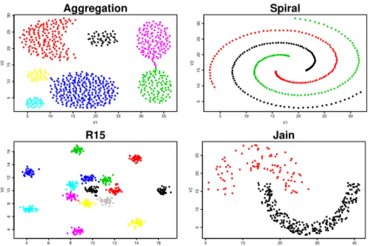
1) Synthetic datasets: The datasets which have been chosen are (see Fig. 1):
• Aggregation (Ag) [21]: This dataset is composed by 7 clusters, some of them can be separated by parametric clustering.
• Jain(Jn) [22]: This dataset is composed by two surfaces with different density and a clear separation.
• R15[23]: This dataset is divided in 15 clusters which are clearer separated.
• Spiral(Sp) [24]: In this case, there are 3 spirals close to each other.
2) Real-World datasets: The datasets which have been chosen have been extracted from the UCI database [25]. They are the following:
• Iris(Ir): Contains 3 classes of 50 instances each, where each class refers to a type of iris plant. Each instance has 4 attributes. This well known dataset has been used in several clustering works [26].
• Wine(Wn): Contains 3 classes with 13 attributes each and 178 instances. It also has been used in some clustering works as [27].
• Glass (Gl): Contains 6 classes with 9 attributes each and 214 instances. It also has been analysed in some clustering works as [28]
• Libras Movement (LM): Contains 15 classes with 90 attributes each and 24 instances per class (total 360). It is identified for classification and clustering in the UCI database [25].
• Ozone Level Detection(OL): Contains 2 classes with 73 attributes and 2536 instances. It has been chosen because of its simplicity according to the number of classes. • Wine Quality (WQ) [29]: Contains 6 classes with 11
attributes each and 4898 instances of white wine. it is also identified for classification and clustering in the UCI database [25].
• Page Block (PB): Contains 5 classes with 10 attributes each and 5473 instances. It has been chosen because of its complexity.
B. Evaluation Techniques and Experimental Setup
The MOGGC algorithm has been compared against different clustering algorithms. These algorithms have been taken from the literature and from our previous work. The classical algorithms which have been chosen are: K-means, Expectation
Maximization and Spectral Clustering. Also, it has been com-pared against the previous implementation of GGC algorithm [8].
The similarity between the clusters have been calculated using the following similarity metric:
sim(Ci, Cj) = 1 2 Pn q=1δ q Ciδ q Cj |Ci| + Pn q=1δ q Ciδ q Cj |Cj| ! (2) wherenis the number of elements,Ci,Cj the clusters which are compared, |Ci| is the number of elements of cluster Ci andδqC
i is the Kroneckerδdefined by:
δCq
i≡δCi(xq) =
0 if xq ∈/Ci
1 if xq ∈Ci
wherexq is an element. The evaluation process has calculated the maximum accuracy for all the algorithms. All of them have been executed 150 times per dataset. The metric which has been used for the evaluation of K-means and EM is the Euclidean Metric defined by:
||xi−xj||= v u u t d X q=1 (xqi −xqj)2 (3) Wherexi= (x1i, . . . , xdi)andxj = (x1j, . . . , xdj).
And the metric for SC, GGC and MOGGC which has been used in the Similarity Matrix Generation is the Radial Basis Function (RBF) defined by [30]:
s(xi, xj) =e−σ||xi−xj||
2
(4) The σ value has been calculated using the approximation method elaborated by Andrew Ng in [13].
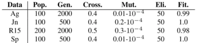
Also, the genetic approaches have been initialized with different parameters. The best parameters for the GAs are shown in Tables I and V for GGC and Tables II and VI for MOGGC. These parameters have been chosen from the experimental results as the best convergence parameters found, nevertheless other parameter choices should obtain similar results. Finally, the Ksize value for MOGGC can be found in Table VIII.
C. Synthetic results for the MOGGC algorithm
Fig. 1 shows the classification results of the different datasets. Table I and Table II show the best fitness values achieved by the GGC and MOGGC algorithms respectively and the parameters selection. In these cases, theσparameter to generate the similarity matrix of the Spectral Clustering, GGC and MOGGC algorithms is 100 (it has been approximated using the method described by Ng et al. [13]). The best accuracy results have been selected for the algorithms.
MOGGC and GGC correctly classify Aggregation. GGC achieves a fitness value of 0.99 which is the maximum value of fitness achieved by the algorithm (it might be a consequence of those elements which could belong to two clusters) and MOGGC achieves a fitness value of 1.0 for both, Data
Data Pop. Gen. Cross. Mut. Eli. Fit.
Ag 100 2000 0.4 0.01-10−4 50 0.99
Jn 100 500 0.4 0.2-10−4 50 1.0
R15 200 2000 0.5 0.3-10−4 50 0.98
Sp 100 500 0.4 0.01-10−4 50 1.0
TABLE I: Best parameter selection (Population, Generations, Crossover probability, Mutation probability and Elitism size) used in GGC algorithm for the different real datasets and the best fitness value obtained. The tournament size is 2.
Continuity Degree and Clusters Separation which means that the continuity of the information of each clusters is high and also the differences between the clusters. EM, Kmeans and SC have problems related to the form of the data. These problems could be a consequence of local minimum convergence in the search space.
Spiralsis impossible to classify using parametric algorithms and the Euclidean distance (in this case, K-means and EM). This dataset is a perfect example for continuity-cluster separa-tion algorithms such as SC, GGC or MOGGC, for that reason, all of them achieve the best accuracy values (see Table III) with the highest fitness in GGC and MOGGC (see Tables I and II).
Jain is also difficult for parametric techniques. It produces low accuracy values for EM and K-means compared with SC, GCC and MOGGC. This dataset is usually used to test continuity-clustering algorithm modifying the density of the clusters, in this case, the first clusters has a clearly lower data density than the second. These non-parametric algorithms (including SC) have been designed to deal with this kind of problems as the accuracy and fitness results shows.
Finally, theR15 dataset is a good election to test MOGGC algorithm as a parametric algorithm. The results for this dataset shows that EM obtains the best results from classical algorithms. SC obtains worse results than EM due to the noisy information of the clusters, which cover the center of the image (see Fig. 1). MOGGC and GGC obtain the maximum accuracy values, however, the fitness values are lower than in the previous problems (see Tables I and II). GGC fitness value might be a consequence of the noisy information because the clusters are closed to each other. That should be the reason because MOGGC has lower cluster separation (0.98). The continuity degree is also lower (0.87) than in the other cases, it must be because some instances of the clusters are separated from the rest.
This synthetic analysis gives some intuitions about the effec-tiveness of the MOGGC algorithm and the similarity between its results and GGC results. The following experiments will check the efficiency on real-world datasets.
D. Real-world results for the MOGGC algorithm
This section shows the results of the MOGGC algorithm applied to real world datasets. First, it is focused on the preprocessing phase of the datasets. Next, the experimental
5 10 15 20 25 30 35 5 10 15 20 25 30 V1 V2 Aggregation 5 10 15 20 25 30 5 10 15 20 25 30 V1 V2 Spiral 4 6 8 10 12 14 16 4 6 8 10 12 14 16 V1 V2 R15 0 10 20 30 40 5 10 15 20 25 V1 V2 Jain
Fig. 1: Results ofGGCandMOGGCalgorithms. From left to right and from top to bottom: “Aggregation”, “Spiral”,“R15” and “Jain”.
Data Pop. Gen. Cross. Mut. Eli. Fit. DC Fit. CS
Ag 1000 200 0.1 0.01-10−4 50 1.0 1.0
Jn 100 200 0.4 0.03-10−4 10 1.0 1.0
R15 100 2000 0.4 0.01-10−4 50 0.87 0.98
Sp 1000 200 0.4 0.03-10−4 50 1.0 1.0
TABLE II: Best parameter selection (Population, Generations, Crossover probability, Mutation probability and Elitism size) used in MOGGC algorithm for the different real datasets and the best fitness value obtained. The tournament size is 7.
results obtained from MOGGC are compared against to the classical algorithms considered and GGC.
1) Preprocessing: The preprocessing process is divided in two steps:
• The first step has been related to the study of the available variables through histograms and correlation diagrams which were used for dimension reduction. The informa-tion provided by this phase shows the values which are useless because, for example, are constants or have a high correlation (more than 0.85 if we consider that the correlation values is in range [0,1]) with other variables. This means that they may variate the clustering results, if they are not eliminated, with redundant information. Those elements with missing values have been also deleted. Table IV shows the reduction results for the datasets which have been reduced for both correlated
Data K-means EM SC GGC MOGGC
Ag 86.29% 78.68% 88.66% 100% 100% Jn 78.28 % 56.83% 100% 100% 100% R15 80.50 % 99.66% 81.33% 100% 100% Sp 34.61 % 34.93% 100% 100% 100% TABLE III: Best accuracy values obtained by each algorithm using the synthetic datasets.
Data I. Attributes F. Attributes I. Elements F. Elements
LM 90 18 360 360
OL 73 28 2536 1867
TABLE IV: Datasets reduced in the preprocessing process. This table shows the Initial Attributes and Elements with the Final Attributes and Elements after the reduction process
attributes and elements with missing values.
• The second preprocessing phase consists on the normal-ization of the variables. First, the attributes with outliers are recentralized. After, the same range is applied for all. We combine Z-score [31] to recentralized the distribution and avoid outliers and MinMax [32] to fixed the range of all the values between 0 and 1.
Iris (Ir), Wine (Wn), Glass (Gl), Wine Quality (WQ) and
Page Block (PB) datasets contain a few number of attributes. After the analysis of the variables, the correlation shows that the dimensionality reduction is not necessary. However, in the case of Libras Movement (LM) and Ozone Level Detection
(OL) datasets there are a lot of attributes which do not contribute to the analysis due to the high correlation between them (see Table IV). These attributes have been reduced in the first step leaving 18 of 90 attributes for Libras Movement and 28 of 73 for Ozone Level Detection. In the Ozone Level Detection datasets, there are several instances which contain missing values, all these instances have been omitted for the analysis (see Table IV).
All the attributes from the datasets considered have been normalized applying the techniques of the second step.
2) Results: The experiments have followed the same proce-dure that was made in the synthetic datasets experiments. The value of σ has been approximated to 100 for Iris, Wine and
Glass, 2 forLibras MovementandOzone Level Detectedand 0.1 for Wine Qualityand Page Block. The results are shown in Table VII.
The results for theIris show that EM is the best classifier (with an accuracy of the 96,67%), MOGGC is the second (96%) and the GGC algorithm is the third (92%), it could be due Iris dataset has instances of different classes which are closed to each other, the GGC algorithm has problems to discriminate the boundary of the clusters specially when there are intersections between the clusters. This problem also affects to MOGGC algorithm. The fitness achieved by GGC and MOGGC is high in both cases (see Table V and VI), it means that the solution of the algorithm should be the best solution they are able to find.
The results for the Wine datasets shows that all the algo-rithm obtain high accuracy values (higher than the 95%), and the Genetic Algorithms obtain a perfect classification with the maximum fitness value for GGC and maximum Cluster Separation for MOGGC. These results are a consequence of the data distribution, the classes are clearer separated than in the Iris case (as the different clustering techniques show). It improves the results of the GGC and MOGGC algorithms,
Data Pop. Gen. Cross. Mut. Eli. Fit. Ir 1000 2000 0.1 0.8-10−4 50 0.99 Wn 100 20000 0.4 0.01-10−4 50 1 Gl 100 2000 0.4 0.01-10−4 10 0.70 LM 100 2000 0.01 0.01-10−4 10 0.92 OL 100 200 0.4 0.01-10−4 10 0.93 WQ 1000 2000 0.4 0.01-10−4 10 0.80 PB 100 20000 0.4 0.01-10−4 50 0.92
TABLE V: Best parameter selection (Population, Generations, Crossover probability, Mutation probability and Elitism size) used in GGC algorithm for the different real datasets and the best fitness value obtained. The tournament size is 2.
because the boundary is clearer.
Glass dataset is a difficult classification case, the results show that both, the classical and the new algorithms have problems to blindly separate the classes. In this case, SC obtains the best classical algorithm results while GGC obtains the same value of SC and MOGGC obtains the best results. However, the fitness metrics values are low for both which means that they might find other solutions in the search space although these solutions are those with higher fitness of the experimental tests.
Libras Movements dataset is also a difficult classification case, again the classical and the new algorithms have problems to blindly separate the classes. In this case, SC obtains the best results from the classical algorithms while GCC and MOGGC obtain the same results. However, the fitness metrics values are still low for both.
Ozone Level Detectedis easier for the continuity-clustering algorithms. In this case, SC, GCC and MOGGC obtain the best classification results.
Wine Qualityis a difficult problem for clustering techniques. The worst results are achieved by the parametric algorithms (the accuracy is lower than the 30%). The results of the non-parametric techniques are the same. MOGGC has a high value of the Clusters Separation fitness, which means that this solution is closed to the best solution that it is able to find. In the case of GGC, the fitness is 0.80, it means that the algorithm might be able to find others solutions although this value was the best convergence value reached by the algorithm.
Page Block is also a difficult problem for parametric ap-proximation and a good memory efficiency example. The parametric algorithms have achieved low accuracy results while SC and MOGGC have achieved the same solutions. These results show that GGC and MOGGC have achieved the best solution according to the Cluster Continuity metric, however, in this case, the Continuity Degree Value is smaller than usual. Analysing the parametric clustering results, they show that the data instances within the clusters should be separated between them instead of have a clear union between them.
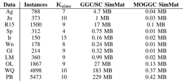
E. The memory optimization of the Similarity Graph
Table VIII shows how the new MOGGC algorithm improves the storage of the Similarity Graph related to the SC, GGC and
Data Pop. Gen. Cross. Mut. Eli. Fit. CD Fit. CS
Ir 1000 2000 0.1 0.1-10−4 50 0.99 0.99 Wn 1000 2000 0.3 0.1-10−4 50 0.89 1 Gl 100 100 0.5 0.01-10−4 10 0.83 0.70 LM 100 200 0.5 0.01-10−4 10 0.91 0.65 OL 100 200 0.5 0.01-10−4 10 0.92 1 WQ 100 20000 0.4 0.01-10−4 50 0.88 0.99 PB 1000 10000 0.4 0.2-10−4 50 0.43 1
TABLE VI: Best parameter selection (Population, Generations, Crossover probability, Mutation probability and Elitism size) used in MOGGC algorithm for the different real datasets and the best fitness values obtained. The tournament size is 7.
Data K-means EM SC GGC MOGGC
Ir 89.33% 96.67% 89.33% 92% 96.00% Wn 95.50% 97.19% 95.50% 100% 100% Gl 45.79% 47.20% 47.20% 47.20% 47.66% LM 46.94% 43.61% 46.11% 50.00% 50.00% OL 76.06% 60.15% 94.38% 96.46% 96.46% WQ 23.64% 28.50% 40.08% 40.08% 40.08% PB 45.30% 56.97 % 75.15% 75.15% 75.15% TABLE VII: Best accuracy values obtained by each algorithm during the experimental results applied to the UCI datasets.
MOGGC algorithms. There are some cases where the memory efficiency is highly relevant such as Ozone Level Detection,
Wine Quality and Page Block. Specially, in the Page Block
problem, the matrix takes up the 0.2% of the original matrix. This important improvement joined with the performance efficiency, makes the algorithm highly competitive against other approaches.
V. CONCLUSIONS ANDFUTUREWORK
This work proposes MOGGC, a new clustering algorithm, inspired by GGC, that introduces Multi-Objective Genetic Algorithms. MOGGC uses a simple codification and GA-based operations combined with the SPEA2 algorithm. In comparison to GGC, the new algorithm requires less memory while, at the same time, increases the quality of the evolved clusters. MOGGC is applied to a reduced version of the Similarity Graph which is generated in the first step of the
Data Instances Ksize GGC/SC SimMat MOGGC SimMat
Ag 788 7 4.7 MB 0.04 MB Jn 373 10 1 MB 0.03 MB R15 1500 9 17 MB 0.1 MB Sp 312 4 0.75 MB 0.01 MB Ir 150 15 0.16 MB 0.02 MB Wn 178 8 0.24 MB 0.01 MB Gl 214 9 0.32 MB 0.01 MB LM 360 9 0.99 MB 0.02 MB OL 1867 9 27 MB 0.13 MB WQ 4898 10 183 MB 0.37 MB PB 5473 10 229 MB 0.42 MB TABLE VIII: Storage GGC and MOGGC. In this case it is supposed that the Similarity Matrix is a matrix of double
Spectral Clustering algorithm. The results, given in Section IV, show that the new algorithm obtains excellent results that are better than the classical algorithms, and has a similar (or better) classification results than previous obtained using GGC, while the memory usage is clearly optimized.
The future work will be focused on several improvements that could be made to the MOGGC algorithm. On the one hand, the effects of noisy information should be deeply analysed, whereas on the other hand the number of clusters could be automatically selected using strategies such as cross-validation. Finally, other fitness functions which could improve the MOGGC algorithm convergence, and the clusters quality, could be studied.
ACKNOWLEDGMENT
This work has been partly supported by: Spanish Ministry of Science and Education under project TIN2010-19872.
REFERENCES
[1] I. Yoo and X. Hu, “A comprehensive comparison study of document clustering for a biomedical digital library medline,” inProceedings of the 6th ACM/IEEE-CS joint conference on Digital libraries, ser. JCDL ’06. New York, NY, USA: ACM, 2006, pp. 220–229.
[2] P. Haider, L. Chiarandini, and U. Brefeld, “Discriminative clustering for market segmentation,” inProceedings of the 18th ACM SIGKDD international conference on Knowledge discovery and data mining, ser. KDD ’12. New York, NY, USA: ACM, 2012, pp. 417–425. [3] A. Pascual, M. Barc´ena, J. Merelo, and J.-M. Carazo, “Application of the
fuzzy kohonen clustering network to biological macromolecules images classification,” in Engineering Applications of Bio-Inspired Artificial Neural Networks, ser. Lecture Notes in Computer Science, J. Mira and J. S´anchez-Andr´es, Eds. Springer Berlin Heidelberg, 1999, vol. 1607, pp. 331–340. [Online]. Available: http://dx.doi.org/10.1007/BFb0100500 [4] G. Bello-Orgaz, M. D. R-Moreno, D. Camacho, and D. F. Barrero, “Clustering avatars behaviours from virtual worlds interactions,” in Proceedings of the 4th International Workshop on Web Intelligence; Communities. New York, NY, USA: ACM, 2012, pp. 4:1–4:7. [5] D. MacKay, Information Theory, Inference and Learning Algorithms.
Cambridge University Press, 2003.
[6] A. P. Dempster, N. M. Laird, and D. B. Rubin, “Maximum Likelihood from Incomplete Data via the EM Algorithm,”Journal of the Royal Statistical Society. Series B (Methodological), vol. 39, no. 1, pp. 1–38, 1977.
[7] U. von Luxburg, “A tutorial on spectral clustering,” Statistics and Computing, vol. 17, no. 4, pp. 395–416, Dec. 2007.
[8] H. Men´endez and D. Camacho, “A genetic graph-based clustering algorithm,” inIntelligent Data Engineering and Automated Learning -IDEAL 2012, ser. Lecture Notes in Computer Science, H. Yin, J. Costa, and G. Barreto, Eds. Springer Berlin / Heidelberg, 2012, vol. 7435, pp. 216–225.
[9] D. T. Larose,Discovering Knowledge in Data. John Wiley & Sons, 2005.
[10] S. E. Schaeffer, “Graph clustering,”Computer Science Review, vol. 1, no. 1, pp. 27–64, 2007.
[11] C. Coello, G. Lamont, and D. Van Veldhuisen,Evolutionary Algorithms for Solving Multi-Objective Problems, ser. Genetic and evolutionary computation series. Springer Science+Business Media, LLC, 2007. [12] E. Hruschka, R. Campello, A. Freitas, and A. de Carvalho, “A survey of
evolutionary algorithms for clustering,”Systems, Man, and Cybernetics, Part C: Applications and Reviews, IEEE Transactions on, vol. 39, no. 2, pp. 133 –155, march 2009.
[13] A. Ng, M. Jordan, and Y. Weiss, “On Spectral Clustering: Analysis and an algorithm,” inAdvances in Neural Information Processing Systems, T. Dietterich, S. Becker, and Z. Ghahramani, Eds. MIT Press, 2001, pp. 849–856.
[14] Coley, An Introduction to Genetic Algorithms for scientists and engi-neers. World Scientific Publishing, 1999.
[15] K. Deb and D. Kalyanmoy,Multi-Objective Optimization Using Evolu-tionary Algorithms, 1st ed. Wiley, Jun. 2001.
[16] A. Mukhopadhyay, S. Bandyopadhyay, and U. Maulik, “Clustering using multi-objective genetic algorithm and its application to image segmentation,” inSystems, Man and Cybernetics, 2006. SMC ’06. IEEE International Conference on, vol. 3, Oct., pp. 2678–2683.
[17] J. Lee, L. Choi, and S. Park, “Multi-objective genetic algorithms, nsga-ii and spea2, for document clustering,” inSoftware Engineering, Business Continuity, and Education, ser. Communications in Computer and Information Science, T.-h. Kim, H. Adeli, H.-k. Kim, H.-j. Kang, K. Kim, A. Kiumi, and B.-H. Kang, Eds. Springer Berlin Heidelberg, 2011, vol. 257, pp. 219–227.
[18] E. Zitzler, M. Laumanns, and L. Thiele, “SPEA2: Improving the Strength Pareto Evolutionary Algorithm,” Gloriastrasse 35, CH-8092 Zurich, Switzerland, Tech. Rep. 103, 2001.
[19] K. Deb, S. Agrawal, A. Pratap, and T. Meyarivan, “A fast elitist non-dominated sorting genetic algorithm for multi-objective optimisation: Nsga-ii,” inProceedings of the 6th International Conference on Parallel Problem Solving from Nature, ser. PPSN VI. London, UK, UK: Springer-Verlag, 2000, pp. 849–858.
[20] D. Corne, J. D. Knowles, and M. J. Oates, “The pareto envelope-based selection algorithm for multi-objective optimisation,” in Proceedings of the 6th International Conference on Parallel Problem Solving from Nature, ser. PPSN VI. London, UK, UK: Springer-Verlag, 2000, pp. 839–848.
[21] A. Gionis, H. Mannila, and P. Tsaparas, “Clustering aggregation,”ACM Trans. Knowl. Discov. Data, vol. 1, no. 1, Mar. 2007.
[22] A. Jain and M. Law, “Data clustering: A user’s dilemma,” inPattern Recognition and Machine Intelligence, ser. Lecture Notes in Computer Science, S. Pal, S. Bandyopadhyay, and S. Biswas, Eds. Springer Berlin / Heidelberg, 2005, vol. 3776, pp. 1–10.
[23] C. Veenman, M. Reinders, and E. Backer, “A maximum variance cluster algorithm,” Pattern Analysis and Machine Intelligence, IEEE Transactions on, vol. 24, no. 9, pp. 1273 – 1280, sep 2002.
[24] H. Chang and D.-Y. Yeung, “Robust path-based spectral clustering,” Pattern Recogn., vol. 41, no. 1, pp. 191–203, Jan. 2008.
[25] A. Frank and A. Asuncion, “UCI machine learning repository,” 2010. [Online]. Available: http://archive.ics.uci.edu/ml
[26] A. Likas, N. Vlassis, and J. J. Verbeek, “The global k-means clustering algorithm,”Pattern Recognition, vol. 36, no. 2, pp. 451 – 461, 2003. [27] M. Bilenko, S. Basu, and R. J. Mooney, “Integrating constraints and
metric learning in semi-supervised clustering,” in Proceedings of the twenty-first international conference on Machine learning, ser. ICML ’04. New York, NY, USA: ACM, 2004, pp. 11–.
[28] X. Z. Fern and C. E. Brodley, “Solving cluster ensemble problems by bipartite graph partitioning,” in Proceedings of the twenty-first international conference on Machine learning, ser. ICML ’04. New York, NY, USA: ACM, 2004, pp. 36–.
[29] P. Cortez, A. Cerdeira, F. Almeida, T. Matos, and J. Reis, “Modeling wine preferences by data mining from physicochemical properties,” Decis. Support Syst., vol. 47, no. 4, pp. 547–553, Nov. 2009. [30] S. Ghosh-Dastidar, H. Adeli, and N. Dadmehr, “Principal component
analysis-enhanced cosine radial basis function neural network for robust epilepsy and seizure detection,”Biomedical Engineering, IEEE Trans-actions on, vol. 55, no. 2, pp. 512 –518, feb. 2008.
[31] S. R. Carroll and D. J. Carroll, Statistics Made Simple for School Leaders. Rowman & Littlefield, 2002.
[32] J. Han and M. Kamber,Data mining: concepts and techniques. Morgan Kaufmann, 2006.