UC Irvine Previously Published Works
Title
Predicting floods in a large karst river basin by coupling PERSIANN-CCS QPEs with a
physically based distributed hydrological model
Permalink
https://escholarship.org/uc/item/6nt8x5fx
Journal
HYDROLOGY AND EARTH SYSTEM SCIENCES, 23(3)
ISSN
1027-5606
Authors
Li, Ji
Yuan, Daoxian
Liu, Jiao
et al.
Publication Date
2019-03-15
DOI
10.5194/hess-23-1505-2019
License
https://creativecommons.org/licenses/by/4.0/ 4.0
Peer reviewed
https://doi.org/10.5194/hess-23-1505-2019 © Author(s) 2019. This work is distributed under the Creative Commons Attribution 4.0 License.
Predicting floods in a large karst river basin by coupling
PERSIANN-CCS QPEs with a physically based
distributed hydrological model
Ji Li1, Daoxian Yuan1,2, Jiao Liu3, Yongjun Jiang1, Yangbo Chen4, Kuo Lin Hsu5, and Soroosh Sorooshian5 1School of Geographical Sciences of Southwest University, Chongqing Key Laboratory
of Karst Environment, Chongqing 400715, China
2Karst Dynamic Laboratory, Ministry of Land and Resources, Guilin 541004, China 3Chongqing Hydrology and Water Resources Bureau, Chongqing 401120, China
4Department of Water Resources and Environment, Sun Yat-Sen University, Guangzhou 510275, China 5Center for Hydrometeorology and Remote Sensing, Department of Civil and Environmental Engineering,
University of California, Irvine, Irvine, California
Correspondence:Ji Li ([email protected])
Received: 16 August 2018 – Discussion started: 5 September 2018
Revised: 12 December 2018 – Accepted: 26 February 2019 – Published: 15 March 2019
Abstract. In general, there are no long-term meteorologi-cal or hydrologimeteorologi-cal data available for karst river basins. The lack of rainfall data is a great challenge that hinders the development of hydrological models. Quantitative precipi-tation estimates (QPEs) based on weather satellites offer a potential method by which rainfall data in karst areas could be obtained. Furthermore, coupling QPEs with a distributed hydrological model has the potential to improve the pre-cision of flood predictions in large karst watersheds. Esti-mating precipitation from remotely sensed information us-ing an artificial neural network-cloud classification system (PERSIANN-CCS) is a type of QPE technology based on satellites that has achieved broad research results worldwide. However, only a few studies on PERSIANN-CCS QPEs have occurred in large karst basins, and the accuracy is gener-ally poor in terms of practical applications. This paper stud-ied the feasibility of coupling a fully physically based dis-tributed hydrological model, i.e., the Liuxihe model, with PERSIANN-CCS QPEs for predicting floods in a large river basin, i.e., the Liujiang karst river basin, which has a wa-tershed area of 58 270 km2, in southern China. The model structure and function require further refinement to suit the karst basins. For instance, the sub-basins in this paper are divided into many karst hydrology response units (KHRUs) to ensure that the model structure is adequately refined for karst areas. In addition, the convergence of the underground
runoff calculation method within the original Liuxihe model is changed to suit the karst water-bearing media, and the Muskingum routing method is used in the model to calcu-late the underground runoff in this study. Additionally, the epikarst zone, as a distinctive structure of the KHRU, is care-fully considered in the model. The result of the QPEs shows that compared with the observed precipitation measured by a rain gauge, the distribution of precipitation predicted by the PERSIANN-CCS QPEs was very similar. However, the quantity of precipitation predicted by the PERSIANN-CCS QPEs was smaller. A post-processing method is proposed to revise the products of the PERSIANN-CCS QPEs. The karst flood simulation results show that coupling the post-processed PERSIANN-CCS QPEs with the Liuxihe model has a better performance relative to the result based on the initial PERSIANN-CCS QPEs. Moreover, the performance of the coupled model largely improves with parameter re-optimization via the post-processed PERSIANN-CCS QPEs. The average values of the six evaluation indices change as follows: the Nash–Sutcliffe coefficient increases by 14 %, the correlation coefficient increases by 15 %, the process rela-tive error decreases by 8 %, the peak flow relarela-tive error de-creases by 18 %, the water balance coefficient inde-creases by 8 %, and the peak flow time error displays a 5 h decrease. Among these parameters, the peak flow relative error shows the greatest improvement; thus, these parameters are of the
greatest concern for flood prediction. The rational flood sim-ulation results from the coupled model provide a great prac-tical application prospect for flood prediction in large karst river basins.
1 Introduction
The highly anisotropic karst water-bearing media and intri-cate hydraulic conditions cause karst flood processes to ex-hibit significant differences in time and space, which leads to laminar flow and turbulent flow transmutation in karst ar-eas; thus, flood events in karst river basins are more com-plicated than those in non-karst areas (Ford and Williams, 1989; Goldscheider and Drew, 2007). This difference makes it difficult to precisely simulate and forecast the karst flood process using a hydrological model. It is common practice to simplify karst water-bearing media before building a model. For example, the karst river basin could be made into a multi-ple and nested spatial structure, the underground river could be made into an intelligible river system in the model, and the cave could be an anisotropic medium with a large ver-tical infiltration coefficient and porosity but a small specific yield. Even so, it is still hard to quantify the spatial structure of karst water-bearing media with a physics–mathematics model. Karst flood simulation results usually have some er-rors that cannot be ignored, and these erer-rors represent the main problem in flood prediction in karst river basins (Ko-vacs and Perrochet, 2011).
Because the dynamic changes in karst hydrological pro-cesses and the hydraulic conditions of the underlying sur-face are complicated and nonlinear in karst areas, obtain-ing hydrogeological parameters, such as specific yield, hy-draulic conductivity and aquifer transmissivity, is difficult. With the rapid development of remote sensing, GIS technol-ogy and hydrogeoltechnol-ogy, the technoltechnol-ogy used in field work, in-cluding tracer tests (Birk et al., 2005; Doummar et al., 2012) and infiltration tests, has made significant progress. How-ever, accurately simulating the laws of motion of karst hy-drological processes in karst water-bearing media based on these experimental tests remains difficult. Therefore, tradi-tional methods, such as lumped hydrological models, are not suitable for flood prediction in karst areas (Hartmann et al., 2013). Compared with the performance of lumped hydrolog-ical models, physhydrolog-ically based distributed hydrologhydrolog-ical mod-els (PBDHMs) have some advantages in terms of generat-ing karst flood predictions. PBDHMs divide the entire karst river basin into a series of small grid units named karst sub-streams, which precisely reflect the real rules of hydrologi-cal processes and karst development characteristics. There-fore, the PBDHM approach has great application potential in terms of improving karst flood simulation and prediction capabilities (Ambroise et al., 1996). Many PBDHMs have been proposed since the blueprint of the PBDHM was
pub-lished by Freeze and Harlan (1969). The first full PBDHM, called the SHE model, was published in 1987 (Abbott et al., 1986a, b). Shustert and White (1971) attempted to use the PBDHM in karst areas. In their research, the dissolved car-bonate species were analyzed in the waters of 14 carbon-ate springs in the central Appalachians. These springs were classified into diffuse-flow feeder-system types and conduit feeder-system types. PBDHMs have obtained several good research results in karst areas (Atkinson, 1977; Quinlan and Ewers, 1985; Quinlan et al., 1996; Duan and Miller, 1997; Ren, 2006; Liu et al., 2013; Zhang et al., 2007).
The PBDHM used in this paper is the Liuxihe model (Chen, 2009), which is a fully distributed model with 14 physically based parameters. After the karst mechanisms were added, the number of parameters was 20. Unlike other distributed hydrological models, there are some special struc-tural designs in this model. For instance, the whole model structure is divided into eight independent parts, which are called sub-models. These sub-models include the (1) wa-tershed division and data mining sub-model, (2) unit clas-sification and river section estimation sub-model, (3) rain-fall fusion computational sub-model, (4) evapotranspiration calculation sub-model, (5) runoff calculation sub-model, (6) confluence calculation sub-model, (7) parametric sen-sitivity analysis sub-model, and (8) parameter optimization sub-model. Unlike other distributed models, separate param-eter uncertainty analysis calculations must be performed out-side the model. However, the parametric sensitivity analysis is a fixed module in the Liuxihe model, which means that when the model is built for flood prediction, parametric un-certainty analysis has already been carried out. The paramet-ric uncertainty analysis in the Liuxihe model is based on a multi-parameter sensitivity analysis that was presented by Choi et al. (1999).
In actual flood predictions, people may pay more attention to the flood process at specific points of the river section. For example, focus may be directed at the mouth of the river or the outlet of the basin. These points have special significance in relation to procedures such as flood warnings and evac-uations. Therefore, extracting the flood processes at these points is important and should be given special consideration. In the Liuxihe model, these points are named early warn-ing points, and flood prediction, which is urgently needed in karst areas, can be performed separately at these points. For example, the confluence of underground rivers could be es-tablished through a field survey and a geological borehole test and set as an early warning point because this is a point at which the influence of karst may dominate the runoff pro-cesses.
In addition, the catchment property data for the Liuxihe model, which primarily include the digital elevation model (DEM), land use and soil types, can be easily downloaded from open-access databases for free. Therefore, the Liuxihe model can be built in any area. Though it is not easy to ob-tain the basic data needed to build a distributed hydrological
model in karst areas, only a very small amount of data must be downloaded from the web to build the Liuxihe model, making it a feasible option for flood simulation and predic-tion in karst basins.
The regulation and storage capacity of karst water-bearing media are weak. When the accumulated rainfall exceeds the maximum drainage capacity of the channel during a heavy rain storm, a karst immersion-waterlogging hazard is much more likely to occur. The hazard will become increasingly serious with the intensification of extreme global weather events. Therefore, some effective measures need to be taken to reduce losses caused by floods. For example, effectively and reliably simulating and predicting the karst flood pro-cess using a PBDHM are important non-project measures for flood control. However, there are insufficient rain gauges and long-term meteorological or hydrogeological data avail-able to build a PBDHM in karst river basins classified as ungauged basins. Predictions in ungauged basins (PUBs) are the theme of the international hydrological decade, at the core of which is runoff calculation (Li and Ren, 2009). Therefore, it is more difficult to forecast flood events in karst river basins than in non-karst areas. How to solve the prob-lem of rainfall sources is a key factor in the current karst flood prediction challenge. Quantitative precipitation esti-mates (QPEs) and, particularly, satellite QPE technology, make it possible to obtain reasonable rainfall data in karst areas. However, the current application of QPEs is imma-ture, which results in poor QPE accuracy, and the effect of the karst flood simulation and prediction is also poor.
The development of numerical weather prediction mod-els in recent decades has provided a reasonable and accu-rate QPE product that can be used in karst areas. The cur-rent mainstream QPEs include weather radar QPEs (Del-rieu et al., 2014; Rafieei et al., 2014; Faure et al., 2015), satellite QPEs and radar-merging satellite QPEs (Stenz, 2014; Bartsotas et al., 2017; Goudenhoofdt and Delobbe, 2009; Wardhana et al., 2017). Additionally, precipitation can be estimated from remotely sensed information us-ing artificial neural networks/PERSIANN QPEs (Soroosh et al., 2000; Hirpa et al., 2010; Romilly, 2011; Yang et al., 2007), the dPERSIANN-climate data record/PERSIANN-CDR (Ashouri et al., 2014; Liu et al., 2017; Tan and Santo, 2018; Hussain et al., 2018), and the PERSIANN-cloud clas-sification system/PERSIANN-CCS (Yang et al., 2004, 2007; Mekonnen and Hossain, 2010). Studying the QPE products from meteorological satellites has become a popular topic in rainfall prediction research (Hu et al., 2013).
Many scholars at home and abroad have performed con-siderable research using QPE technology, and they have achieved many acceptable results. However, considerable un-certainty exists in the application of these results, which causes the precision of the QPEs to be low; thus, the precipi-tation result generated from the QPEs may be unsatisfactory. Two effective measures could reduce the uncertainty of QPE results in the karst area. One measure is to match the
appro-priate resolution of the model. The resolution can directly affect the results of the QPEs; thus, if the resolution is too low, then the division of the grid units is too coarse, which causes a considerable error in the rainfall estimates. How-ever, if the resolution is too high, then the meteorological model structure is complicated and unstable. Furthermore, the required computational resources will increase exponen-tially as the model spatial resolution increases (Chen et al., 2017), which leads to a large number of calculations and low efficiency. Therefore, using the appropriate model spa-tial resolution is extremely important in terms of the QPE results. The other measure that affects uncertainty is that the current technology of QPEs still has some systematic errors due to uncertainties in the structure and mathematical algo-rithms. For this reason, when compared with the precipita-tion observed using rain gauges, the results of QPEs have some relative errors, and these errors cause the karst flood simulation results from the coupled model (i.e., those from coupling the QPEs with a PBDHM) to have uncertainties that largely affect the model’s performance. Therefore, the results of the initial QPEs could not be directly used to build the coupled model. In this study, a post-processing method was employed to revise the productions of the PERSIANN-CCS QPEs products, which caused the QPE results to be more credible and receivable.
There have been many studies of PERSIANN-CCS QPEs (Yang et al., 2007). However, most of these studies have been conducted in small non-karst watersheds. In this study, the PERSIANN-CCS QPEs were employed in an attempt to es-timate the rainfall data in a large karst river basin, i.e., the Liujiang karst river basin (LKRB), which has an area of 5.8×10⁴km2 and is located in Guangxi Province, China. Watershed flood prediction relies on a PBDHM as a com-putation tool, while precipitation is the driving force behind the model (Li et al., 2017). This method has the potential to improve the accuracy of karst flood predictions by cou-pling PERSIANN-CCS QPEs with a PBDHM. The PBDHM in this study is the Liuxihe model (Chen, 2009). This study is the first time the Liuxihe model for flood simulation and prediction in karst basins has been used.
Therefore, the model structure and function have been im-proved to suit the requirements of the karst basin. For in-stance, in this study, the entire river basin will be divided into many small sub-basins using the DEM data, and this process is adequate when considering non-karst basins. However, to ensure the effect and accuracy of the model in karst areas, the model structure must be more refined. Thus, in this pa-per, the sub-basins will be further divided into many karst hy-drology response units (KHRUs). The entire karst hydrologi-cal process, including the storage and regulation processes of the epikarst zone and the spatial interpolation of the precip-itation, evapotranspiration and rainfall–runoff, are all calcu-lated based on the KHRUs. Furthermore, in the original Li-uxihe model, the underground layer is treated as an integral unit, and a linear reservoir method is adopted to calculate the
amount of underground runoff. However, because the struc-ture of the karst underground layer is nonlinear, the original linear reservoir method of the Liuxihe model is not appropri-ate. Therefore, in this study, the Muskingum routing method is used to improve the convergence of the underground runoff calculations. Additionally, the epikarst zone, as a distinctive structure of the KHRU, is carefully considered in the model. An exponential decay equation is used to calculate the regu-lation and storage processes in the epikarst zone.
The spatial resolution of the Liuxihe model for the LKRB is 200 m×200 m. The PERSIANN-CCS QPE prod-ucts, which have a spatial resolution of 0.04◦×0.04◦ and a time interval of 30 min, are employed to estimate the precipitation results for the LKRB. The resolution of the PERSIANN-CCS QPEs must be downscaled to the same size as the Liuxihe model before the coupled model can be built. After post-processing, the PERSIANN-CCS QPE products could offer high-precision precipitation results for the LKRB in locations where there is an inadequate number of rain gauges. Additionally, the model performance can be greatly improved by coupling the post-processed PERSIANN-CCS QPEs with the Liuxihe model. A modified PSO algorithm (Chen et al., 2016) is used to optimize the coupled model parameters in this paper, and this method could control the uncertainty of parameterization.
2 Study area and data 2.1 Study area
The LKRB in southern China was selected as the study area for this research. The LKRB is the second largest tributary of the Pearl River and covers three provinces, namely Guizhou, Guangxi and Hunan. The LKRB is the most developed karst area of China, with a drainage area of 58 270 km2 and a channel length of 1121 km. Moreover, the LKRB is a typical karst-mountainous catchment that has experienced frequent flash flooding in past centuries. The peak forest-plain area is the main karst landform on the ground, while the karst conduit and fissure are well developed underground. There are also many complicated underground rivers and springs with large flows (Li, 1996). The karst water-bearing media are highly nonlinear and heterogeneous, which makes it very difficult to simulate and forecast the karst hydrological pro-cess.
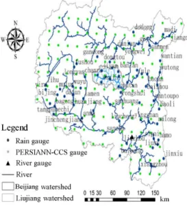
The LKRB is in the sub-tropical monsoon climate zone, with an average annual precipitation between 1400 and 1700 mm, and the precipitation distribution is highly uneven on spatial and temporal scales. The precipitation from April to September accounts for 75 %–80 % of the annual precipi-tation. A sketch map of the LKRB is shown in Fig. 1a.
The most developed karst area in LKRB is the Beijiang catchment, where the influence of karst features highly dom-inates the rainfall–runoff processes. The Beijiang catchment is a tributary of the middle and upper reaches of the Liujiang River, lying at 25◦060–25◦270N and 108◦380–109◦180E. The drainage area of the Beijiang catchment is 1790 km2, and the length is 130 km. The catchment has a dense river system (Fig. 1b) and is surrounded by high mountains with peak el-evation at 1000–1800 m (Fig. 1c), in which the peak-cluster depression covers most of the area. The average valley slope gradient is 0.143.
2.2 Landform, tectonics and hydrogeology information
The LKRB is located in the central part of Guangxi Province, China. The terrain is high on all sides and low in the middle. The cross-strait terraces of the Liujiang River are well de-veloped, especially near the Liuzhou River gauge (as shown in Fig. 1), which is located at the outlet of the LKRB. The northern part of the basin has transmeridional arc-like folded belts, where the soluble rock forms syncline and the sand shale forms anticline. Sand shale formations and carbonate and carbonate clastic rocks are widely distributed here. The karst valley is the main landform in the southern part of the basin, and the overlying lithology is clay and gravel with poor water permeability. The underlying bedrock is mainly carbonate and dolomite, and the karst fissures are well devel-oped, in which a large amount of water is stored (He, 2017). The western part of the basin has a large area of limestone in a continuous distribution, and a peak-cluster depression covers most of the area. The landform of the eastern basin is mainly hilly, where the rocks are soft-hard due to their dif-ferent anti-erosion abilities. The hard rocks form low moun-tains that move towards the gentle slope and then back to the steep slope. The landforms of the central part of the basin are mainly the isolated peak plain and the peak forest plain. Overall, the main landforms of the LKRB are the peak forest plain and the peak-cluster depression.
The Liujiang River is located in the karst valley basin, which is covered by Quaternary loose deposits. The under-lying surface is dominated by alluvium, diluvium and kata-tectic layers due to the fluviraption of the Liujiang River and the karst geological background, and the thickness is approx-imately 10–20 m. Carbonate, sandstone, shale and carbon-ate clastic rocks are widely distributed in the basin. Among them, the area of the carbonate rocks is about 19 230 km2, which accounts for 33 % of the entire watershed. The out-crops in the basin mainly include Upper Devonian lime-stone (D3), Lower Carboniferous Datangpo formation
lime-stone (C1d, C1d3), Middle (C2d) and Upper Carboniferous
(C3) limestone, Upper Permian carbonate and clastic rocks
(P2d, P2 h), Lower Triassic clastic and carbonate rocks (T1),
Lower Cretaceous clastic and carbonate rocks, and loose rock groups of the Quaternary Pleistocene (Q, Qp) and Holocene
Figure 1.Sketch map of Liujiang and the Beijiang catchment.
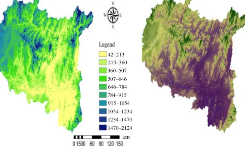
After studying the karst geomorphology of the LKRB, Williams (1987) believed that the peak-cluster depression had developed into turreted peak-forest landforms after a long evolutionary process, which is equivalent to the late prime of life, i.e., entering old age in terms of geomorpho-logic evolution. Allogeneic water, especially from the Liu-jiang River, is the main driving force behind the development of peak-forest landforms. Therefore, the peak-forest plains and valleys are often distributed in contiguous areas near the main trunk stream of the Liujiang River. The main karst land-form of the LKRB is peak-forest plain, and there are also some peak-cluster depressions and peak-forest valleys. Fig-ure 2 shows the DEM and three-dimensional topographical map of the LKRB.
2.3 Rain gauges and karst flood process
There are 68 rain gauges and 131 grid points for the PERSIANN-CCS QPEs within the LKRB, and data from 30 karst flood events that occurred between 1982 and 2013 were collected. There was one flood event each year. Among them, five karst flood events between 2008 and 2013 were used to test the effect of coupling PERSIANN-CCS QPEs with the Liuxihe model. The karst flood process in the LKRB has typical characteristics: the flood peak flows usually exceed 10 000 m3s−1, and there is an expression of a multi-peak flood process. A flood process usually lasts approximately 10 days, and the shortest flood event duration was only ap-proximately 3 days, while the longest was 25 days. Hourly precipitation data were collected from the rain gauges in this
Figure 2.The DEM and three-dimensional topographical map of the LKRB.
study, and these results were compared with the results from the PERSIANN-CCS QPEs. The rain gauges, the grid points of the PERSIANN-CCS QPEs and the Liuzhou River gauge that is located close to the outlet of the LKRB are shown in Fig. 1a.
There are 11 early warning points set in the Beijiang catch-ment (Fig. 1b), and 10 karst flood events at the Goutan warning point were collected to validate the flood simula-tion effect based on the Liuxihe model, in which the Goutan point is the outlet of the Beijiang catchment. In fact, the Beijiang catchment is in the center of the storm area of Guangxi Province, China. According to field observation data, the observed maximum 24 h accumulated precipitation is 779.11 mm in the Beijiang catchment, and the maximum 3-day accumulated precipitation is 1335.15 mm. Karst floods are typical flash floods with rapid discharge and water level fluctuation, mainly caused by storms, and the developed karst landform plays an important role in flood propagation. For instance, the karst depressions can store some water content during heavy rain. Additionally, the regulation functions of the karst fissure system can slow the flood propagation pro-cess.
2.4 Property data
The catchment property data for the distributed hydrological models mainly include the DEM, land use and soil types. These data were downloaded from open-access databases. The DEM was downloaded from the Shuttle Radar Topogra-phy Mission database at http://srtm.csi.cgiar.org (last access: 12 June 2018) (Falorni et al., 2005; Sharma et al., 2014). The downloaded DEM had an initial spatial resolution of 90 m×90 m, and after many model resolution tests, the most
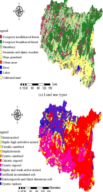
appropriate resolution of the Liuxihe model in the LKRB was confirmed to be 200 m×200 m. Therefore, the spatial resolution of the initial DEM was rescaled to 200 m×200 m in this study, and this value represents the high resolution for the Liuxihe model in the LKRB. The DEM is shown in Fig. 2a. The land use-type data were downloaded from http://landcover.usgs.gov (last access: 12 June 2018) (Love-land et al., 1991, 2000), and the soil-type data were down-loaded from http://www.isric.org (last access: 12 June 2018). The initial spatial resolutions of the land use-type and soil-type data were both 1000 m×1000 m. However, both resolu-tions had to be rescaled to 200 m×200 m in this study. Fig-ure 3a shows the land use types, and b shows the soil types.
3 PERSIANN-CCS QPEs and post-processing results 3.1 PERSIANN-CCS QPEs
The original PERSIANN system (Hsu et al., 1999) was based on geostationary infrared imagery and was later extended to include the use of both infrared and daytime visible imagery. This method represents an automated system for estimat-ing precipitation from remotely sensed information through the use of artificial neural networks. The method for rain-fall estimation that is under development at the University of Arizona is continuously improving as technology advances (Soroosh et al., 2000). The fundamental algorithm of the PERSIANN system is based on a neural network. The net-work parameters could be optimized by an adaptive training characteristic, which can estimate the precipitation from a geosynchronous satellite at any time and place.
Figure 3.The property data for the Liuxihe model in the LKRB.
The PERSIANN-CCS (Yang et al., 2004; Hsu et al., 2007) is a patch-based cloud classification and rainfall estima-tion system from low Earth orbit and geostaestima-tionary satel-lites that uses pattern recognition technology and computer imaging technology (Yang et al., 2007). Satellite-based pre-cipitation retrieval algorithms use information ranging from visible (VIS) to infrared (IR) spectral bands of geostationary earth orbiting (GEO) satellites and microwave (MW) spectral bands (Hsu et al., 2007).
The QPE products of PERSIANN-CCS have generated precipitation estimates at a resolution of 0.04◦×0.04◦scale and at a time interval of 30 min since 2000. The output of
PERSIANN-CCS QPEs was downscaled at 200 m×200 m to achieve the same spatial resolution as that of the Liuxihe model in the LKRB. The down-scaling method used in this paper was based on statistical relationships between the me-teorological variables and DEM data using the LOO (leave-one-out) cross evaluation method and spatial autocorrelation analysis methods (Fan et al., 2017).
The hourly precipitation data from the PERSIANN-CCS QPEs were collected and compared with the precipitation ob-served by the rain gauges.
The estimation of rainfall from the PERSIANN-CCS con-sists of the following steps (Hsu, 2007): (1) IR cloud im-age segmentation, (2) characteristic extraction from IR cloud patches, (3) patch characteristic classification, (4) obtain-ing the rainfall estimation results of the QPE products, and (5) evaluating and revising the results of the QPE products.
In this paper, the PERSIANN-CCS QPEs real-time data used in the LKRB from the current version of PERSIANN-CCS are available and downloadable online (http://cics.umd. edu/ipwg/us_web.html, last access: 28 June 2018).
3.2 Precipitation estimation results
The QPE product of the PERSIANN-CCS generated precip-itation results for the LKRB. There were 131 grid points of PERSIANN-CCS QPEs within the LKRB, and these points were representative and completely covered the entire wa-tershed (as shown in Fig. 1). The spatial resolution was 200 m×200 m, and the time interval was 1 h. The respec-tive QPE products of the PERSIANN-CCS in 2008, 2009, 2011, 2012 and 2013 were produced, and the results indi-cated that five rainfall events corresponded to the five karst flood processes. Figures 4–8 show the average precipitation pattern comparisons of the two precipitation products of the 5 years, where (a) is the average precipitation based on data from the rain gauges, (b) is the average precipitation based on the data from the PERSIANN-CCS QPEs, and (c) is the quantile–quantile plot, in which the 45◦line is used to com-pare two precipitation products.
According to the results of Figs. 4–8, it appears that the temporal average precipitation patterns of both products are quite similar, especially in terms of the rainfall distribution, while there are some differences in the quantitative values. The results from the PERSIANN-CCS QPEs are smaller than those from the rain gauges, which means that a relative error exists between the two products. From the quantile–quantile plot, the two rainfall scatter plots are closely distributed on both sides of the 45◦line, which means that the rainfall
dis-tributions of both products are close to each other.
3.3 Evaluation of PERSIANN-CCS QPEs
To quantitatively evaluate the results of the PERSIANN-CCS QPEs, the precipitation from the PERSIANN-CCS QPEs and the precipitation from the rain gauges were compared in this
Figure 4. Precipitation pattern comparison of two precipitation products (2008): (a) is the average precipitation of rain gauges,
(b)is the average precipitation of PERSIANN-CCS QPEs, and(c)is the quantile–quantile plot, in which the 45◦line is used to compare the two precipitation products.
Figure 5. Precipitation pattern comparison of two precipitation products (2009): (a) is the average precipitation of rain gauges,
(b)is the average precipitation of PERSIANN-CCS QPEs, and(c)is the quantile–quantile plot, in which the 45◦line is used to compare the two precipitation products.
Figure 6. Precipitation pattern comparison of two precipitation products (2011):(a) is the average precipitation of rain gauges,
(b)is the average precipitation of PERSIANN-CCS QPEs, and(c)is the quantile–quantile plot, in which the 45◦line is used to compare the two precipitation products.
Figure 7. Precipitation pattern comparison of two precipitation products (2012):(a) is the average precipitation of rain gauges,
(b)is the average precipitation of PERSIANN-CCS QPEs, and(c)is the quantile–quantile plot, in which the 45◦line is used to compare the two precipitation products.
Figure 8. Precipitation pattern comparison of two precipitation products (2013): (a) is the average precipitation of rain gauges,
(b)is the average precipitation of PERSIANN-CCS QPEs, and(c)is the quantile–quantile plot, in which the 45◦line is used to compare the two precipitation products.
Table 1.Precipitation pattern comparison of the two precipitation products.
Floods Type Average Relative precipitation bias % (mm) 200806090200 rain gauge 1.37 PERSIANN-CCS QPEs 1.22 −11 200906090800 rain gauge 0.74 PERSIANN-CCS QPEs 0.62 −16 201106010900 rain gauge 0.42 PERSIANN-CCS QPEs 0.39 −7 201206022000 rain gauge 0.78 PERSIANN-CCS QPEs 0.63 −19 201306011400 rain gauge 0.53 PERSIANN-CCS QPEs 0.43 −20 average value rain gauge 0.77
PERSIANN-CCS QPEs 0.66 −14
study. The rainfall distribution of both products is shown in Figs. 4–8. For further comparison, the average precipitation of the five karst flood events was calculated, and the results are shown in Table 1.
According to the results of Table 1, there are obvious rela-tive errors between the two precipitation products. The aver-age precipitation values of the PERSIANN-CCS QPEs were lower than those from the rain gauges. For the five karst flood events from 2008 to 2013, the relative errors between the two products were−11 %,−16 %,−7 %,−19 % and−20 %, re-spectively. The average relative error was −14 %, and the maximum error was−20 %, which means that these relative errors cannot be ignored. Therefore, the precipitation results generated by the PERSIANN QPEs must be revised effec-tively, and the precipitation data observed by the rain gauges can be used to revise the results of the PERSIANN QPEs in this study.
3.4 The post-processed PERSIANN-CCS QPEs
To make the results of the PERSIANN QPEs more credible and receivable, the precipitation results were revised using the observed precipitation measured by the rain gauges. First, it was necessary to locate the grid points of the PERSIANN-CCS QPEs that were closest to the rain gauges (as shown in Fig. 1). There were 23 grid points in the LKRB. Second, the average precipitation values of the PERSIANN-CCS QPEs and the rain gauges were calculated, and the average precipi-tation from the rain gauges was used as the true precipiprecipi-tation value. Third, the process of revising the results of the PER-SIANN QPEs based on the average precipitation observed by the rain gauges is summarized as follows.
1. The average precipitation of these 23 grid points based on the PERSIANN-CCS QPEs was calculated with the following equation: PPERSIANN−CCS= N P i=1 PiFi N , (1)
wherePPERSIANN−CCS is the average precipitation of
the 23 grid points based on the PERSIANN-CCS QPEs, Pi is the precipitation based on the PERSIANN-CCS
QPEs at theigrid point,Fiis the catchment area of the igrid point, andN is the number of grid points. 2. The average precipitation of the 23 rain gauges was
cal-culated using the following equation:
P2= M P j=1 Pj M , (2)
whereP2is the average precipitation observed by the
23 rain gauges,Pjis the precipitation observed at thej
rain gauge, andMis the number of rain gauges. 3. The precipitation values observed by the adjacent
PERSIANN-CCS QPEs with the following equation: Pi0=Pi
P2
PPERSIANN−CCS
, (3)
where Pi0 is the value of precipitation based on the PERSIANN-CCS QPEs after revision on the i grid point, andP2/PPERSIANN−CCSis the revised factor.
4. After revision, the precipitation results based on the PERSIANN-CCS QPEs were used as input data for the Liuxihe model to test its feasibility for use in the flood simulation.
After running the post-processing procedure for the PERSIANN-CCS QPEs described above, it was determined that the revised factor P2/PPERSIANN−CCS was a key
fac-tor that made the results of the PERSIANN-CCS QPEs much closer to the value of observed precipitation recorded by the rain gauges, indicating that the systematic errors of the PERSIANN-CCS QPEs could be corrected effectively. Therefore, the post-processing method described in this pa-per is both feasible and necessary. Additionally, it could greatly improve the accuracy of the coupled model in the simulation and prediction of karst floods. Furthermore, the revised factor could be preserved as an empirical value for future flood prediction in the LKRB.
4 Hydrological model 4.1 Liuxihe model
The Liuxihe model proposed by Yangbo Chen (Chen, 2009) of Sun Yat-Sen University, China, is employed as the fully distributed hydrological model in this study, which is a physi-cally based distributed hydrological model (PBDHM) mainly for catchment flood simulation and prediction (Chen et al., 2016, 2017; Li et al., 2017). The Liuxihe model earned its name by being the first successful application in the Liuxihe catchment, Guangdong Province, China. There are three lay-ers vertically, including the canopy layer, the soil layer and the underground layer in the model, and the whole catchment is divided into a great number of grid cells horizontally using the high-resolution DEM data, with the divisions called sub-basins. Each grid is considered a uniform basin, and the ele-vation, land cover type, soil type, and other model elements including rainfall–runoff, evapotranspiration, etc. are calcu-lated in the uniform basin. All cells are categorized into three types, namely hillslope cell, river cell and reservoir cell.
An improved PSO algorithm (Chen et al., 2016) is em-ployed to optimize the model parameters in this study, which can make the model’s performance much better in flood pre-diction in karst river basins. The observed meteorological and hydrological data and the development conditions of the karst underground river are used to optimize the model pa-rameters. The terrain property data, such as the DEM, land
use type and soil type, can be downloaded freely from an open-access database online. The model is validated against observed karst flood events. These factors of the model are physically based and rational to truly reflect the underlying surface of the karst basin. Therefore, this implies that the Li-uxihe model could be used for real-time flood prediction in karst river basins. Figure 9 shows the structure of the Liuxihe model.
4.2 Improvement of the Liuxihe model
The Liuxihe model has been successfully applied for flood predictions in many river basins. However, none of these basins were karst areas. This study is the first time the model has been used in a karst river basin. The structure of the model should be improved to suit the needs of the karst basin in question. Therefore, some effective measures should be taken before building the model. First, the karst water-bearing media should be simplified, and this process could include making the karst basin a multiple and nested spatial structure. The underground river could be included as the in-telligible channel system in the model, and the cave could be used as the anisotropic medium with a large vertical infil-tration coefficient and porosity but a small specific yield. Fi-nally, the fault could be used as the anisotropic medium with a large vertical infiltration coefficient and a specific yield. Second, the entire karst river basin can be divided into many small karst sub-basins using high-resolution DEM data. Fur-thermore, to suit the karst area, the karst sub-basins can be divided into many KHRUs, which are generally independent of each other. The entire karst hydrological process, includ-ing the storage and regulation processes of the epikarst zone, the spatial interpolation of precipitation, the evapotranspira-tion and the rainfall–runoff, are all calculated based on this KHRU. Then, these hydrological processes can be summa-rized for each of the karst sub-basins. Additionally, the out-let flow is formed through the river confluence among each karst sub-basin from the upstream region to the downstream region. This type of multi-structure distributed hydrological model could utilize variously scaled information effectively and optimize the use of observed meteorological, hydrologi-cal and geologihydrologi-cal data.
In this study, the KHRUs were divided by GIS technol-ogy combined with karst topography, land use type and soil type (Ren, 2006). Each KHRU in this study had its own model characteristics, such as meteorological and hydrologi-cal characteristics, as well as the karst developmental char-acteristics. The KHRU was proposed to describe the spa-tial variation of the karst sub-basins. The differences within the KHRUs were smaller than those among the KHRUs. Then, each KHRU was vertically divided into five layers: the canopy, the soil, the epikarst zone, the bedrock and the underground river. A sketch map of the KHRU is shown in Fig. 10.
Figure 9.The structure of the Liuxihe model.
In Fig. 10b, the three-dimensional model of the KHRU in the LKRB was built in the laboratory to better understand how groundwater moves in the karst media and converges with the surface river. Then, the hydrological model could be built and visualized in this way.
To satisfy the applicability of the model in karst areas, the epikarst zone, which is a distinctive structure of the KHRU, was carefully considered in the model. The epikarst zone is composed of karst rocks with macro cracks and tiny fissures. When rain falls on the ground, it is intercepted by plants, held in depressions and experiences some evapotranspira-tion. Then, the rainfall infiltrates into the soil and rock layer and satisfies the water shortage of the unsaturated zone. Part of the water in the epikarst zone may form karst springs that emerge from the surface. Another part will enter the superfi-cial karst water system of the epikarst zone. When the rainfall intensity is heavy enough to form surface runoff on the ex-posed bedrock, part of the water will enter the karst conduit through sinkholes.
The karst hydrological process of the epikarst zone could be divided into rapid fissure flow and slow fissure flow. After heavy rain, a large amount of water in the epikarst zone is stagnant and can form a surface karst aquifer with a tempo-rary water table. If there are large cracks or fractures under
the water table, a precipitation funnel will form and be as-sociated with a drop in the water table. Rapid fissure flow refers to rainfall that infiltrates into the karst conduit through the precipitation funnel, and this flow occurs in the macro cracks and has high speeds. When rainfall enters the superfi-cial karst water system of the epikarst zone, the macro cracks will fill first. This part of the saturated water content, named rapid fissure flow, will move directly into the karst conduit through the macro crack. Because this rapid fissure flow will pass quickly through the karst conduit system without stop-ping, and because the water regulation and storage functions are weak, the regulation and storage of the rapid fissure flow were ignored in this study. The rest of the water content in the epikarst zone infiltrates through tiny fissures. This part of the water, named slow fissure flow, plays an important role in the process of rainfall regulation. The water content of the slow fissure flow can be described by the following equation: SWepi=Qinf−Vcrk, (4)
where SWepiis the water content of the slow fissure flow in
the epikarst zone.
Qinf is the infiltration water content of the rainfall, and
Vcrkis the water content of the rapid fissure flow in the macro
Figure 10.Sketch map of the KHRU.
The slow fissure flow in the epikarst zone is calculated by an exponential decay equation (Ren, 2006) as follows:
Wsep=Wepi 1−exp −1T TTperc , Wepi, t+1=Wepi, t+SWepi, t+1−Wsep, t+1,
TTperc=
SATepi−FCepi
Kepi
,
(5)
whereWsepis the water content that flows from the epikarst
zone to the underground river. Because the regulation and storage functions of the rapid fissure flow are ignored in this study,Wseprefers to the slow fissure flow,Wepiis the current
water content of the slow fissure flow in the epikarst zone (where subscripted epi stands for epikarst, and the same ap-plies below),1T is the simulation time step, TTperc is the
attenuation coefficient, SATepiis the saturation water content
of the slow fissure flow, FCepiis the field capacity, andKepiis
the saturated hydraulic conductivity of the slow fissure flow. The linear reservoir model is employed to calculate the regulation process of the superficial karst fissure system in the epikarst zone, and the base discharge is calculated by the hydraulic gradient of the KHRU (Neitsch et al., 2002) as fol-lows: Qgw=8000 Kepihwt bl Lgw2 , Qgw, i=Qgw, i−1exp −agw1t, +Wrchrg1−exp −agw1t, Wrchrg, i=Wseep 1−exp − 1 δgw , +Wrchrg, i−1exp − 1 δgw , (6)
whereQgwis the base discharge,Qgw, iandQgw, i−1are the
supply quantities of the base discharge that converges into
the karst conduit or underground river on theiday and the (i−1) day, respectively,Kepiis the saturated hydraulic
con-ductivity of the epikarst zone,hwt blis the hydraulic gradient, Lgwis the length of the KHRU,agw is the depletion
coeffi-cient of the base discharge,1T is the simulation time step (day),Wrchrg, i is the supply quantity of the aquifer on the iday (mm d−1),Wseepis the water flux through the bottom
of the soil profile into the underground aquifer on thei day (mm d−1), andδgwis the delay time of the supply (day).
In the original Liuxihe model, the underground layer is treated as an integral unit, and a linear reservoir method is used to calculate the underground runoff. However, the struc-ture of the karst underground layer is nonlinear; thus, the linear reservoir method is obviously not appropriate here. Therefore, in this study, the Muskingum routing method was used to calculate the convergence process of the karst under-ground river, and the equation is as follows:
W=K[xI+(1−x)O] =KO0, (7) whereO0 is the water storage content,O is the outlet flow of the river reach,xis the dimensionless proportion factor,I is the inflow discharge of the river reach, andKis the slope of the correlation curve of the water storage content and the discharge.
The finite difference method is used to calculate the water balance equation and the Muskingum routing method:
O2=C0I2+C1I1+C2O1,
C0+C1+C2=1,
where C0= 0.51t−Kx 0.51t+K−Kx, C1= 0.51t+Kx 0.51t+K−Kx, C2= −0.51t+K−Kx 0.51t+K−Kx . (9)
If the Muskingum routing method parameters of K and x can be determined for a karst underground river reach, then the values of C0,C1 andC2 can be calculated by Eq. (6).
When1t=2Kx,C0=0, which means that the karst flood
prediction lead time will be 2Kx. Under this condition, the Muskingum routing method can be simplified as follows: O2=C1I1+C2O1. (10)
One of the key problems of the Muskingum routing method involves determining how to optimize the parametersKand xin practical applications. It is hard to generalize the param-etersKandxin flood simulation and prediction due to their variability with flow conditions. Ahilan et al. (2012) used the generalized extreme value (GEV) to analyze the flood fre-quency distributions in Irish rivers, and the result showed that a Type II distribution appears in a single cluster in the karst area, which reflects the finite nature of karst storage and the effects of saturation when storage is no longer available. In this study, 30 karst flood events are collected to validate the performance of the Muskingum model in study area. The least squares method is used to optimize the parameters K andxin this study as follows:
min ( E= n X j=1 {W0(j )−W1(j )−C}2 ) , (11)
whereEis the objective function between the observed wa-ter storage content and the simulated wawa-ter storage content, which requires only the least squares approximation with re-gard to the functional value; W0(j )andW1(j ) are the
ob-served and simulated water storage contents within thej pe-riod, respectively;W1(j )=K[xI+(1−x)O];nis the total
number of observation periods; and C is the absolute value of the water storage content.
To simplify the calculation,A=K·xandB=K·(1−x); then, the partials can be taken with respect toA, B, andC, respectively: PW 0I =API2+BP(OI )+CPI2, P W0O=AP(OI )+BPO2+CPO, P W0I =API+BPO+Cn. (12)
Then, the values ofA, B,andCcan be calculated as follows:
A=y1 y2 −y3 y2 , B=y1z2 y3z2 −y2z1 y2z3 , C=PW0−A P I−BP O n , (13) where y1=P(W0I )− P W0PI n , y2=PI2− P I2 n , y3=P(I O)− P OP I n , z1=P(W0O)− P W0PO n , z2=PO2− P O2 n , z3=PI O− POP I n , K=A+B, x=K A. (14)
The parameters of the Muskingum routing method can be optimized using the equations shown above. Then, the con-vergence process of the karst underground river can be cal-culated by the Muskingum routing method in the Liuxihe model.
5 Model setup
5.1 Hydrological model setup
The method that combines a DEM with a stream network leads to a more accurate drainage network in terms of surface runoff modeling (Li and Tao, 2000), especially in karst areas. In this study, based on the high resolution of 200 m×200 m used for the Liuxihe model in the LKRB, the entire studied area was divided into 1 469 900 grid cells, which were named the karst sub-basins, using the DEM. The grid cells included 1 463 204 hillslope cells and 6696 river cells. Then, the karst sub-basins were further divided into many KHRUs. The river system was divided into 3 orders as shown in Fig. 1.
Because of the sinkholes and karst depressions in the karst watershed, as well as the systematic error of the DEM it-self, there are many pits, including true and false pits, in the LKRB. Among them, the true pits include karst depressions and sinkholes, and they usually have a certain scale and ele-vational differences. The false pits were represented only by a few points with low elevation, which was due to the sys-tematic errors of the DEM. Therefore, the true and false pits should be reliably distinguished before using the DEM data to divide the area into the karst sub-basins. First, we identi-fied all of the pits with low elevation and connected them on a plane. Then, we distinguished the true pits from the false pits based on the on-site topographic survey. Finally, the model retained the true pits such as the sinkholes and karst depres-sions, but the false pits were filled (i.e., removed).
The KHRU was introduced in this study to reasonably de-scribe the spatial variability of the karst water-bearing media (as shown in Fig. 10). The spatial characteristics of every
KHRU have a definite physical meaning. Therefore, the cal-culation of the evapotranspiration, rainfall runoff and param-eter optimization of the KHRU was physically based, which could truly reflect the differences of the underlying surface. After the division of the karst sub-basins and the KHRUs, the post-processed PERSIANN-CCS QPE results can be used as the input data for the Liuxihe model to simulate and fore-cast the karst flood process. The performance of the coupled model was reliably improved in this way.
In the Liuxihe model, the flood process of specific points, named the early warning points of some critical river sec-tions, could be simulated and predicted. Figure 1 shows that there are few rain gauges located upstream of the Liujiang River (which is why the PERSIANN-CCS QPEs were used here). However, the karst is very developed here, and the in-fluence of the karst dominates the runoff processes. There-fore, an early warning point was established at the Goutan River gauge (Fig. 1b) to extract the most developed karst area in the LKRB, Beijiang catchment, where the influence of karst features highly dominates the rainfall–runoff pro-cesses. There are 11 early warning points set in the Beijiang catchment (Fig. 1b).
5.2 Parameter optimization of the coupled model
There were 14 parameters that needed to be optimized for the original Liuxihe model, and after adding the karst mech-anism, the number of parameters increased to 20, as shown in Table 2. The parameters of the epikarst zone were the most complicated due to the anisotropy of the karst water-bearing media, which made it difficult to measure and calculate the hydraulic characteristics.
The hydrogeology parameters used in this study, includ-ing the permeability coefficient of the rock mass, the rainfall infiltration coefficient, the specific yield of the aquifer, and the storage coefficient, were calculated by the field test and the experience function. For instance, the permeability coef-ficientKwas calculated by an experience function according to the water inrush prediction of a coal mine in the study area:
Q=1.366K(2H−M)·M−h 2 lgR0−lgr0 · 1 24, R0=r0+10·S √ K, r0= r a·b π , (15)
whereQis the mine inflow, m3h−1;K is the permeability coefficient, m d−1;His the distance from the water-resisting
floor to the water level of the confined aquifer, m;Mis the aquifer thickness, m; h is the height of the dynamic water level, m; R0 is the substitute influence radius, m;r0 is the
substitute radius, m;Sis the drawdown value, m; anda·bis the area of the mine, m2.
In the water inrush test of the coal mine, the other param-eters in Eq. (15) were given, and the permeability coefficient Kwas calculated by anti-Eq. (15).
The parameters of the epikarst zone, including the thick-ness, saturated water content, field capacity and macro crack volume ratio, were obtained based on the field survey, geo-logical borehole test and pumping test as well as on the em-pirical value observed in the study area.
The epikarst zone was mainly developed on the hard sur-face of pure carbonate rock, especially on Paleozoic lime-stone. The thicknesses and characteristics of the epikarst zone differ due to different climates, topography and land-forms. The parameters of the coupled model and the epikarst zone are listed in Table 2a and b, and the rainfall infiltra-tion coefficients of the different karst landforms are calcu-lated based on the empirical values shown in Table 2c.
The soil type parameters, such as the saturated water con-tent and the field capacity, were calculated using a software tool (Ren, 2006). The statistical relationship between the soil texture and the soil water can be easily queried in the software tool. In addition, this method has been effectively proven by many experiments (Servat and Sakho, 1995), and the calculated value of this method has a good fitting rela-tionship with the measured value.
The Liuxihe model has been deployed on a supercomputer system with parallel computation technology (Chen et al., 2016). An improved PSO algorithm (Chen et al., 2017) was employed to optimize the parameters of the coupled model in this study. There are 30 karst flood events from 1982 to 2013 in the LKRB, and among them, 3 flood events – Floods 2004070300, 2009060908, and 2011010100 – were used for parameter optimization simulations in this paper. The flood simulation results are shown in Fig. 11 and Table 3.
From the flood simulation results in Fig. 11, it can be seen that the Flood 2009060908 simulated result is the best. The simulated process for this flood is closest to the observed pro-cess, and the valuation indices of flood simulation results in-cluding the Nash–Sutcliffe coefficient,C; correlation coeffi-cient,R; process relative error,P%; peak flow relative error, E%; coefficient of water balance,W; and peak time error, T(h), are also the best. Table 3 shows the valuation indices of flood simulation results from the improved PSO algorithm. Therefore, Flood 2009060908 is finally adopted for the Liux-ihe model parameter optimization. Other floods will be used to verify the model performance.
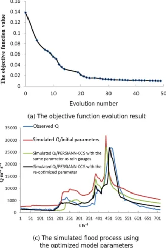
The parameter optimization results from the improved PSO algorithm are shown in Fig. 12 as follows: (a) the objec-tive function evolution result, (b) the parameter evolution re-sult, and (c) the simulated flood process using the optimized model parameters.
To test the parameter optimization effect with differ-ent precipitation sources, both the precipitation of the rain gauge and the precipitation of the PERSIANN-CCS QPEs were used to optimize the parameters of the coupled model. For comparison, the simulated flood process of the cou-pled model with the same parameter from the rain gauges and the re-optimized parameter from the post-processed PERSIANN-CCS QPEs are drawn in Fig. 12c.
Table 2.The parameters of the model.
(a)The parameters of the coupling model.
Parameter types Name Variable Physical property Sensitivity Adjustability name
Evapotranspiration Potential evaporation Ep Meteorology insensitive adjustable
Evaporation coefficient λ Vegetation type medium sensitive adjustable Wilting percentage Cwl Vegetation type insensitive adjustable
The epikarst zone Thickness h Soil type and Karst sensitive unadjustable rock property
Saturated water content θsat Soil type highly sensitive adjustable
Saturation permeability coefficient θs Soil type highly sensitive adjustable
Macro crack volume ratio V Karst rock property highly sensitive adjustable Field capacity θfc Soil type sensitive adjustable
Rainfall–runoff Soil layer thickness z Soil type sensitive adjustable Saturated hydraulic conductivity Ks Soil type highly sensitive adjustable
Soil coefficient b Soil type sensitive adjustable Flow direction Fd Landform highly sensitive unadjustable
Slope S0 Landform highly sensitive unadjustable
Bottom slope Sp Landform sensitive adjustable
Bottom width Sw Landform sensitive adjustable
Slope roughness n Landform and sensitive adjustable Vegetation type
Channel roughness n1 Landform and sensitive adjustable
Vegetation type
The underground Depletion coefficient ω Landform and medium sensitive adjustable
river Soil type
Muskingum routing method/ K Landform highly sensitive adjustable The slope of the water storage
content and flow curve
Muskingum routing method/ χ Landform highly sensitive adjustable the proportion of the flow
(b)The physical parameters of the epikarst zone
Thickness/h(m) Saturated water content/ Saturation permeability Macro crack volume Field capacity/
θsat(g cm−3) coefficient/θs(mm h−1) ratio/V (m3m−3) θfc(mm)
3–10 0.12–0.3 100–420 0.05–0.15 0.16-0.3
(c)The rainfall infiltration coefficient of different karst landforms
Landforms karst strongly karst moderately karst poorly developed developed developed
closed depression 0.6–0.8 0.4–0.6 0.15–0.18 not closed depression 0.4–0.7 0.3–0.5 0.18–0.2 monadnock, platform 0.2–0.3 0.2–0.3 0.2–0.25 gully, slope 0.01–0.2 0.01–0.2 0.01–0.2
Table 3.The evaluation indices of flood simulation results obtained through parameter optimization by the improved PSO algorithm.
Floods Nash– Correlation Process Peak flow The coefficient Peak time Sutcliffe coefficient/R relative relative of water error/T(h) coefficient/C error/P% error/E% balance/W
2004070300 0.78 0.82 0.23 0.08 0.85 −8
2009060908 0.95 0.92 0.17 0.04 0.09 −5
2011010100 0.8 0.84 0.26 0.03 1.02 −7
Figure 11.The flood simulation results obtained through parameter optimization by the improved PSO algorithm.
5.3 Parametric uncertainty analysis
In this study, parametric uncertainty analysis refers to sen-sitivity analysis, and this process is conducted using a fixed module called the parametric sensitivity analysis sub-model in the Liuxihe model. It is a parameter sensitivity analysis method that was developed based on the GLUE method, and it was named multi-parameter sensitivity analysis (MPSA) by Choi et al. (1999). Monte Carlo sampling was used to obtain the value of the parameter spatial variation. The sen-sitivity of each parameter could be obtained by running the model multiple times.
In this study, the Nash–Sutcliffe coefficient was used as the objective function value for the parametric sensitivity analy-sis, and the formula is as follows:
NSE=1− n P i=1 Qi−Q0i2 n P i=1 Qi−Q 2, (16)
where NSE is the objective function value of the Nash– Sutcliffe coefficient,QiandQ0i are the observed streamflow
and the simulated streamflow, respectively, in m3s−1,Qis the average value of the observed flows in m3s−1, andnis the number of observation periods in h.
First, the initial value range of the parameter was deter-mined to be [0.5, 2.5]. Second, 6000 groups of parameter se-quences were obtained by the Monte Carlo sampling method. Third, the Liuxihe model was run to simulate the objective function values of the Nash–Sutcliffe coefficient, and the karst flood processes were the three flood events also used for parameter optimization. In this study, the critical value of the Nash–Sutcliffe coefficient was 0.85, and the objec-tive function values below this threshold were considered to be unacceptable values; otherwise, they were considered to be acceptable values. The degree of separation between these values indicates the sensitivity of the parameters. This degree of separation was calculated according to the Nash– Sutcliffe coefficient (NSD). To analyze parameter sensitivity more easily, a factor SI is given here, and SI=1− |NSD|– the closer the value of SI is to 0, the less sensitive the pa-rameter. Table 4 shows the SI values, which represent the sensitivity of the parameters in the Liuxihe model.
6 Results and discussion
6.1 Results of parameter optimization and sensitivity analysis
The results of the parameter optimization are shown in Fig. 12 as follows: (a) the objective function evolution re-sult and (b) the parameter evolution rere-sult. From the rere-sults of Fig. 12a and b, it can be seen that the evolution num-ber of the objective function for the parameter was 50, and the computation time of the parameter optimization based on the improved PSO algorithm was approximately 8 h, which means that convergence of the parameter optimization was achieved after only 50 cycles. In comparison, the computa-tion time of the initial model parameters that were not op-timized was approximately 55 h. This result implies that the improved PSO algorithm had high efficiency in terms of pa-rameter optimization.
To test the parameter optimization effect using the im-proved PSO algorithm (Chen et al., 2017), the flood
pro-Figure 12.Parameter optimization results with the improved PSO algorithm.
cess simulated results achieved from the improved PSO al-gorithm, as well as the initial model parameter values, are shown in Fig. 12c. From the results shown in Fig. 12c, it can be seen that the coupled model does not simulate the ob-served karst flood process well when the initial model param-eter values are used. Additionally, the simulated flood pro-cess obtained from using the improved PSO algorithm was very close to that from the observed process, which means that the improved PSO algorithm (Chen et al., 2017) in this study was effective and could largely improve the perfor-mance of the coupled model.
In this study, the sensitivity of the parameters in the Liux-ihe model was calculated according to the Nash–Sutcliffe co-efficient, as shown in Eq. (16). The values of SI=1− |NSD|, which represent the sensitivity of the parameters, and the re-sults in Table 4 indicate that the SI values of the saturated water content parameter,θsat, were maximized, which means
that the degree of separation between the unacceptable val-ues and the acceptable valval-ues (NSD) was minimal. This pa-rameter,θsat, was the most sensitive parameter in the Liuxihe
model. When the SI value of a parameter is greater than 0.7, this parameter is identified as a highly sensitive parameter in the Liuxihe model, and SI values between 0.2 and 0.7 indi-cate that a parameter has medium sensitivity. When the SI
value is less than 0.2, the parameter is insensitive. From Ta-ble 4, the SI values of the different parameters, from largest to smallest, are the saturated water content,θsat>saturation
permeability coefficient, θs>field capacity, θfc>saturated
hydraulic conductivity, Ks>macro crack volume ratio,
V >Muskingum routing method (the slope of the water storage content and flow curve), K>Muskingum routing method (the proportion of the flow),χ >soil layer thickness, z>soil coefficient, b>bottom width, Sw>bottom slope,
Sp>slope roughness,n>channel roughness,n1>depletion
coefficient,ω>evaporation coefficient, λ>potential evapo-ration,Ep>wilting percentage, andCwl. Additionally, the
θsat,θs,θfc,Ks,V,K, andχ parameters were highly
sen-sitive; thez,b,Sw,Sp,n,n1andωparameters had medium
sensitivity; and theλ,Ep, andCwlparameters were
insensi-tive.
The flow direction, slope and thickness parameters of the epikarst zone could not be adjusted. Among them, the flow direction and the slope were directly calculated by the DEM data, and the thickness of the epikarst zone was a fixed value for a particular region. It was approximately 3–10 m of the study area according to the field survey.
Table 4.The calculation results of the parameter sensitivity in the Liuxihe model. Floods Potential evaporation/Ep Evaporation coefficient/λ Wilting per-centage/Cwl Saturated water content/θsat Saturation permeability coefficient/θs Macro crack volume ratio/V Field capacity/θfc Soil layer thickness/z Saturated hydraulic conductivity/Ks 2004070 0.06 0.08 0.02 0.92 0.90 0.77 0.85 0.68 0.82 30000 Soil coefficient/b Bottom slope/Sp Bottom width/Sw Slope roughness/n Channel roughness/n1 Depletion coefficient/ω Muskingum routing method/The slope of the water storage content and flow curve/K Muskingum routing method/the proportion of the flow/χ 0.65 0.36 0.49 0.27 0.19 0.12 0.76 0.75 2009060 90800 Potential evaporation/Ep Evaporation coefficient/λ Wilting per-centage/Cwl Saturated water content/θsat Saturation permeability coefficient/θs Macro crack volume ratio/V Field capacity/θfc Soil layer thickness/z Saturated hydraulic conductivity/Ks 0.08 0.11 0.05 0.96 0.92 0.81 0.89 0.65 0.87 Soil coefficient/b Bottom slope/Sp Bottom width/Sw Slope roughness/n Channel roughness/n1 Depletion coefficient/ω Muskingum routing method/The slope of the water storage content and flow curve/K Muskingum routing method/the proportion of the flow/χ 0.62 0.54 0.58 0.32 0.25 0.12 0.78 0.78 2011060 10900 Potential evaporation/Ep Evaporation coefficient/λ Wilting per-centage/Cwl Saturated water content/θsat Saturation permeability coefficient/θs Macro crack volume ratio/V Field capacity/θfc Soil layer thickness/z Saturated hydraulic conductivity/Ks 0.12 0.25 0.07 0.89 0.82 0.71 0.79 0.62 0.75 Soil coefficient/b Bottom slope/Sp Bottom width/Sw Slope roughness/n Channel roughness/n1 Depletion coefficient/ω Muskingum routing method/The slope of the water storage content and flow curve/K Muskingum routing method/the proportion of the flow/χ 0.58 0.52 0.55 0.48 0.42 0.33 0.72 0.68
6.2 Model validation results
To better test the effect of the Liuxihe model in flood simula-tion and predicsimula-tion and to increase the results’ acceptability, 30 karst flood events from 1982 to 2013 in LKRB are simu-lated by the Liuxihe model, and the evaluation indices of the simulated flood results are listed in Table 5. Table 5 shows that the six evaluation indices of the flood simulation results for the 30 flood events are credible and reasonable. The av-erage value of the Nash–Sutcliffe coefficient (C) is 0.82, the correlation coefficient (R) is 0.83, the process relative error (P) is 0.22, the peak flow relative error (E) is 0.05, the water balance coefficient (W) is 0.87, and the peak flow time error (T) is−6 h. Among these results, the peak flow relative er-ror (E) is minimal. The applicability of the Liuxihe model is proven through these accepted flood simulation effects in the LKRB.
To further validate the performance of the Liuxihe model in flood simulation and prediction, simulations are performed in a very developed karst area, where the influence of karst landforms plays an important role in hydrological processes. The most developed karst area in the whole basin exam-ined in this study is the Beijiang catchment, and it is di-vided by the early warning point Goutan set in the Liuxihe model (Fig. 1b). In total, 10 karst flood events are simulated to test the performance of the Liuxihe model, and the evalu-ation indices of the simulated flood results are shown in Ta-ble 6. From these results, four karst flood simulation results are shown in Fig. 13.
From the results in Table 6, the evaluation indices of the simulated karst flood results produced by the Liuxihe model are quite good in the Beijiang catchment. The average value of the Nash–Sutcliffe coefficient (C) is 0.92, the correlation coefficient (R) is 0.91, the process relative error (P) is 0.11, the peak flow relative error (E) is 0.08, the water balance
Table 5.The evaluation indices of the simulated flood results based on the Liuxihe model in the LKRB.
Floods Nash– Correlation Process Peak flow The Peak Sutcliffe coefficient/ relative relative coefficient time coefficient/ R error/ error/ of water error/
C P% E% balance/W T (h) 1982081219 0.84 0.75 0.3 0.01 0.83 −4 1983020308 0.82 0.84 0.21 0.04 0.89 −5 1984010100 0.75 0.89 0.26 0.14 0.96 −3 1985010100 0.73 0.87 0.17 0.01 1.05 −5 1986010100 0.83 0.85 0.23 0.04 0.94 4 1987050100 0.93 0.76 0.1 0.05 1.01 −6 1988051620 0.84 0.8 0.15 0.04 0.9 −8 1989042600 0.64 0.74 0.39 0.02 0.88 −5 1990050100 0.85 0.87 0.14 0.03 0.85 −3 1991053118 0.8 0.76 0.25 0.04 0.95 10 1992042900 0.66 0.84 0.2 0.11 0.89 5 1993060900 0.91 0.89 0.24 0.09 1.05 −8 1994060700 0.93 0.85 0.14 0.04 0.85 −6 1995052100 0.82 0.7 0.2 0.01 0.81 −10 1996060600 0.9 0.93 0.18 0.02 0.86 −5 1997060400 0.84 0.87 0.13 0.06 0.95 −4 1998051600 0.83 0.85 0.3 0.01 1.05 −6 1999061700 0.6 0.83 0.15 0.05 0.8 −5 2000052100 0.79 0.89 0.26 0.06 0.83 −8 2001051500 0.8 0.82 0.25 0.07 0.82 −6 2002042600 0.86 0.9 0.24 0.02 0.87 −2 2003060600 0.92 0.85 0.14 0.04 0.76 −4 2004070300 0.78 0.82 0.23 0.08 0.85 −8 2005061400 0.76 0.76 0.35 0.06 0.74 −5 2006060400 0.82 0.83 0.3 0.1 0.86 −3 2008060900 0.8 0.91 0.15 0.03 0.89 −6 2009060908 0.95 0.92 0.17 0.04 0.09 −5 2011010100 0.8 0.84 0.26 0.03 1.02 −7 2012010100 0.82 0.79 0.2 0.05 0.8 −6 2013010100 0.95 0.82 0.2 0.06 0.92 −4 mean value 0.82 0.83 0.22 0.05 0.87 −6
Table 6.The evaluation indices of the simulated flood results based on the Liuxihe model in the Beijiang catchment.
Floods Nash– Correlation Process Peak flow The Peak flow Sutcliffe coefficient/ relative relative coefficient time coefficient/ R error/ error/ of water error/
C P% E% balance/W T (h) 2000101512 0.89 0.92 0.11 0.09 0.93 −3 2003091014 0.91 0.88 0.13 0.11 0.89 −2 2005070815 0.93 0.89 0.09 0.13 0.95 2 2008071311 0.97 0.89 0.08 0.09 0.95 −1 2010081012 0.87 0.93 0.12 0.07 0.91 −4 2012080310 0.9 0.95 0.06 0.05 0.96 2 2013091210 0.92 0.91 0.09 0.09 0.89 3 2014061015 0.93 0.93 0.18 0.07 1.08 −2 2015091008 0.93 0.89 0.13 0.08 0.92 −3 2016091501 0.94 0.9 0.11 0.04 0.92 1 mean value 0.92 0.91 0.11 0.08 0.94 3
Figure 13.Karst flood simulation results from the Liuxihe model in the Beijiang catchment.
coefficient (W) is 0.94, and the peak flow time error (T) is 3 h. It is obvious that the evaluation indices of the simulated karst flood events based on the Liuxihe model are satisfying, and the accuracy is very high.
Additionally, from the flood simulation results in Fig. 13, the four reasonable karst flood simulation results, includ-ing those for Floods 2008071311, 2012080310, 2014061015, and 2016091501, prove the performance of the Liuxihe model in karst areas. The simulated flood discharge pro-cesses are very close to the observed values, especially for the peak flows. This finding implies that the Liuxihe model is feasible and effective in flood simulation and prediction in areas where karst is very well developed, as in the Beijiang catchment.
6.3 Results of flood simulation with the post-processed PERSIANN-CCS QPEs
After the correction was made, the post-processed PERSIANN-CCS QPE precipitation became much closer to the precipitation observed at the rain gauge. To analyze the effects of flood simulation with the initial PERSIANN-CCS QPEs and the post-processed QPEs, five karst flood events, including Floods 200806090200, 200906090800, 201106010900, 201206022000 and 201306011400, were simulated and compared; the results are shown in Fig. 14. In this simulation, the coupled model parameters remained unchanged; i.e., the original coupled model parameters based
on the rain gauge precipitation were employed, while the re-optimized model parameters based on the precipitation of the post-processed PERSIANN-CCS QPEs were not.
Figure 14 shows that the karst flood simulation results from the initial PERSIANN-CCS QPEs were not satisfac-tory, and the performance of the model was worse than that of the rain gauge precipitation. For instance, the simulated peak flows from the PERSIANN-CCS QPEs were lower than the observed peak flows. The performance of the coupled model with the post-processed PERSIANN-CCS QPEs was much better, and the evaluation indices of the flood simula-tion were largely improved (as shown in Table 7). The av-erage value of the Nash–Sutcliffe coefficient (C) increased by 7 %, the correlation coefficient (R) increased by 8 %, the process relative error (P) decreased by 6 %, the peak flow relative error (E) decreased by 14 %, the water balance co-efficient (W) increased by 5 %, and the peak flow time error (T) had a decrease of 2 h. Among these parameters, the peak flow relative error had the largest improvement, making it the most important factor in flood prediction. It was obvious that the evaluation indices improved substantially when the post-processed QPEs were used. Therefore, the post-processing method for PERSIANN-CCS QPEs in this paper was fea-sible and effective. In addition, coupling the post-processed PERSIANN-CCS QPEs with the Liuxihe model has the po-tential to improve the model performance in flood simulation and prediction in the LKRB.