Analysis and Simulation of Scheduling Techniques for Real-Time Embedded Multi-core Architectures

Institute of Software Technology

Department of Programming Languages and Compilers University of Stuttgart

Universit¨atsstraße 38 D–70569 Stuttgart

Master Thesis Nr. 3578

Analysis and Simulation of

Scheduling Techniques for

Real-Time Embedded Multi-core

Architectures

Sanjib Das

Course of Study: INFOTECH

Examiner: Prof. Dr. rer. nat./Harvard Univ. Erhard Pl ¨odereder Supervisor: Dipl.-Inf. Mikhail Prokharau

Commenced: October 31, 2013 Completed: June 27, 2014

Abstract

In this modern era of technological progress, multi-core processors have brought significant and consequential improvements in the available processing potential to the world of real-time embedded systems. These improvements impose a rapid increment of software complexity as well as processing demand placed on the underlying hardware. As a consequence, the need for efficient yet predictable multi-core scheduling techniques is on the rise.

As part of this thesis, in-depth research of currently available multi-core scheduling tech-niques, belonging to both partitioned and global approaches, is done in the context of real-time embedded systems. The emphasis is on the degree of their usability on hard real-time systems, focusing on the scheduling techniques offering better processor affinity and the lower number of context switching. Also, an extensive research of currently available real-time test-beds as well as real-time operating systems is performed.

Finally, a subset of the analyzed multi-core scheduling techniques comprising PSN-EDF, GSN-EDF, PD2 and PD2∗ is simulated on the real-time test-bed LITMUSRT.

Acknowledgments

First and foremost, I offer my sincerest obligation to honorable Prof.Dr.rer.nat./Harvard Univ. Erhard Pl¨odereder for giving the opportunity to write my master’s thesis at Department of Programming Languages and Compilers of the Institute of Software Technology at the University of Stuttgart.

Moreover, I would like to show my humble gratitude to my supervisor Dipl.-Inf. Mikhail Prokharau who has supported me throughout my thesis with his knowledge, cordial supervision, valuable pieces of advice and patience while at the same time giving me the room to work in my own way.

I am profoundly grateful to my parents Jatindra Nath Das and Shikha Das for their uncon-ditional support and constant encouragement throughout my life.

In addition, it is my pleasure to express gratefulness to all the people who contributed, in whatever manner, to the success of this work.

Contents

Abbreviations 1 1 Introduction 3 1.1 Motivation . . . 3 1.2 Objective . . . 3 1.3 Organization . . . 4 2 Definitions 7 2.1 A Real-Time System . . . 7 2.2 An Embedded System . . . 7 2.3 Multi-Core Systems . . . 7 2.4 Task Models . . . 8 2.5 Resource . . . 10 2.6 Scheduling Policy . . . 10 2.7 Schedulers . . . 11 3 Terminology 13 3.1 Schedulability and Optimality of scheduling algorithm and Feasibility of tasksets 13 3.2 Processor Demand Bound Function . . . 13

3.3 Utilization Bound . . . 13

3.4 Resource Augmentation or Speedup Factor . . . 13

4 Classification of Scheduling Algorithms for Multi-Core Systems 15 5 Related Work on Real-time Scheduling Techniques 19 5.1 Partitioned Approach . . . 19

5.1.1 Tasksets consist of Implicit Deadlines . . . 19

5.1.2 Tasksets consist of Constrained and Arbitrary Deadlines . . . 21

5.2 Global Approach . . . 21

5.2.1 Global Scheduling with Fixed Job Priority . . . 22

5.2.2 Global Fixed Task Priority Scheduling . . . 22

5.2.3 Global Dynamic Priority Scheduling . . . 24

5.3 Summary . . . 31

6 Related Work on Real-time Scheduling Test-beds 33 6.1 Linux-kernel . . . 34 6.2 Kernel Preemption . . . 34 6.3 RTLinux . . . 35 6.4 S.Ha.R.K . . . 36 6.5 MaRTE . . . 36 6.6 RTAI . . . 36 6.7 Xenomai . . . 37 6.8 XtratuM/PaRTiKle . . . 38 6.9 ChronOS . . . 39 6.10 LITMUSRT . . . 40

6.11 Summary . . . 41

7 Simulation 43 7.1 Baseline Platform . . . 44

7.2 Experimental Task Sets . . . 46

7.3 Algorithm Implementation . . . 47

7.4 Experiment Results . . . 48

7.5 Summary . . . 54

8 Conclusion and Future Work 57

List of Figures

2.1 Real-Time Task Parameter Buttazzo [2004] . . . 8

2.2 Task State Diagram Buttazzo [2004] . . . 10

2.3 Task queue in Scheduler Buttazzo [2004] . . . 11

4.1 Categories of real-time scheduling algorithms [Mohammadi and Akl, 2005] . . . . 15

5.1 A periodic task τi containing 11 subtasks with Ui = ₁₁8 representing the group deadline of subtask τi,j [Nelissen et al., 2014] . . . 27

5.2 Pfair and BFair schedules of three tasksτ0, τ1andτ2, where number of processors ism= 2. The periods areT0 = 15, T1 = 10, T2 = 30,and the worst-case execution times areC0 = 10, C1= 7, C2= 19,[Nelissen et al., 2014] . . . 30

6.1 RTLinux Architecture [Yiqiao et al., 2008] . . . 35

6.2 RTAI Architecture [Yiqiao et al., 2008] . . . 37

6.3 Xenomai Architecture [Yiqiao et al., 2008] . . . 38

6.4 XtratuM/PaRTiKle Architecture [Yiqiao et al., 2008] . . . 39

6.5 ChronOS Architecture [ChronOS, 2013] . . . 40

7.1 Plugin . . . 48

7.2 Context switching (µs) and scheduling overheads (µs) of PD2 as PFAIR and PD2∗ as PFAIR23 algorithms with very-light processor utilization distribution for tasksets with task number increasing from 5 to 100 in steps of 5 . . . 51

7.3 Context switching (µs) and scheduling overheads (µs) of PD2 as PFAIR and PD2∗_{as PFAIR23 algorithms with full range processor utilization distribution for} tasksets with task number increasing from 5 to 100 in steps of 5 . . . 52

7.4 Context switching (µs) and scheduling overhead (µs) of PSN-EDF,GSN-EDF,C-EDF,PFAIR,PFAIR23 algorithms for tasksets with tasks increasing from 5 to 100 in steps of 5, utilization distribution: full range . . . 53

7.5 Record loss rations (%) of PSN-EDF,GSN-EDF,C-EDF,PFAIR,PFAIR23 algo-rithms for tasksets with tasks increasing from 5 to 100 in steps of 5, utilization distribution: full range. . . 54

List of Tables

7.1 Simulation platform configuration of virtual and physical machines . . . 46 7.2 Uniform distribution of utilization used in task set generation . . . 46 7.3 Simulation data of PD2on QEMU emulator with uni-very-light processor

utiliza-tion distribuutiliza-tion and 24 tasks . . . 49 7.4 Simulation data of PD2∗ on QEMU emulator with uni-very-light processor

uti-lization distribution and 24 tasks . . . 49 7.5 Simulation data of PD2 on physical machine with uni-very-light processor

utiliza-tion distribuutiliza-tion and 24 tasks . . . 50 7.6 Simulation data of PD2∗ on physical machine with uni-very-light processor

uti-lization distribution and 24 tasks . . . 50 7.7 Number of context switches incurred for PD2 and PD2∗ with the taskset of 24

Abbreviations

CFS Completely Fair Scheduler

DM Deadline Monotonic Scheduling

EDF-BF Earliest Deadline First - Best Fit EDF-FF Earliest Deadline First - First Fit

FPU Floating-Point Unit

G-EDF Global Earliest Deadline First

GSN-EDF Global Suspendable Non-Preemptive EDF

GUA Global Utility Accrual

IPC Interposes communication

NMIs Non Maskable Interrupts

NUMA Non-uniform memory access

P-EDF Partitioned Earliest Deadline First Pfair Proportionate Fairness

POSIX Portable Operating System Interface

PSN-EDF Partitioned EDF with synchronization support RMGT Rate Monotonic Scheduler for General Task

RMS Rate Monotonic Scheduler

RMST Rate Monotonic Scheduler for Short Task

RTOS Real Time Operating System

TSC Time Stamp Counter

VFS Virtual File System

1.

Introduction

1.1

Motivation

These days embedded systems are sewn into our day-to-day life in various forms of visible and invisible manner via many different application areas which include consumer electronics, medical imaging, telecommunications, automotive electronics, avionics, space systems, etc. For instance, the progress in use of multi-core platforms in embedded systems has already reached our hands as a form of mobile phones and related devices with small form factor.

The main purpose of a real-time system is to produce the required result within strict time constraints including computational correctness. In other words, in the physical world the purpose is to construct a physical effect within a chosen time-frame [Mohammadi and Akl, 2005]. There are a number of perspectives to classify real-time systems. Depending on the system characteristics, a real-time system can be categorized as hard real-time or soft real-time by considering factors inside the system and factors outside the system [Juvva, 1998].

As many embedded systems are used in safety-critical applications, their correct functionality in the whole system is imperative to avoid severe consequences. It is estimated that 99% of produced microprocessors are integrated into embedded systems [Burns and Wellings, 2001]. Furthermore, as a result of this abrupt technological progress, a significant increment in software complexity and processing demands of real-time systems is seen [Davis and Burns, 2011]. To cope with these processing demands, silicon vendors are concentrating on using multi-core platforms for high-end real-time applications instead of incrementing processor clock speeds in uni-core platforms. By the same token, scheduling research of multi-core architectures offers a broad spectrum of significant opportunities for real-time system producers. [Davis and Burns, 2011] . Research of uni-core and multi-core real-time scheduling both originated back in late 1960s and early 1970s, consequential advances were made in 1980s and 1990s [Davis and Burns, 2011]. Still, there is sufficient scope for research, although uni-core real-time scheduling is considered reasonably mature to be in industrial practice [Burns and Wellings, 2001]. On the other hand, many of well researched multi-core scheduling techniques are not mature enough to either be applicable or optimal as much as currently available uni-core real-time scheduling techniques.

For this reason, reliable simulation platforms are required to augment the research of schedul-ing techniques for real-time embedded multi-core architectures, which is also coupled with an-alytical results that expect guaranteed real-time administration over the system by the most effective use of the available processing capability through employing efficient scheduling poli-cies placed on the underlying hardware.

1.2

Objective

The purpose of this work is to give an overview of currently available real-time embedded multi-core scheduling techniques along with simulation test-beds while giving detailed comparison of their advantages and limitations. Consequently simulate analyzed scheduling techniques on suitable test-bed. The objectives are as categorized as follows:

1. Analysis of scheduling techniques for real-time embedded multi-core architectures

• In-depth analysis of currently available literature on multi-core scheduling in real-time contexts.

1 Introduction

• Comparison of multi-core scheduling techniques, emphasizing the degree of their us-ability on hard real-time embedded systems.

• Comparison of multi-core scheduling techniques by focusing on techniques offering better processor affinity and the lower number of context switching. In-depth analysis, considering above constraints, of the following scheduling policies:

– Partitioned approach (includes Partitioned-EDF)

∗ Tasksets with implicit deadlines including partitioned RMST, partitioned RMGT, EDF-FF, EDF-BF

∗ Tasksets with constrained and arbitrary deadlines including EDF-FFID

– Global approach with

∗ Fixed-job priority including global EDF-US[ς],global EDF(κ)

∗ Fixed-task priority including global RM, global RM-US[ς], global DM-DS, global FP

∗ Dynamic priority including Pfair, PF, ERfair, PD2, PD2∗, BF, BF2, LLREF, EDZL

2. Analysis of currently available simulation test-beds for scheduling techniques for real-time embedded multi-core architectures.

• Analysis and comparison of existing real-time test-beds to evaluate scheduling tech-niques including the following ones:

– RTLinux, – S.Ha.R.K, – MaRTE, – RTAI, – Xenomai, – XtratuM/PaRTiKle, – ChronOS, – LITMUSRT.

• Selection of suitable real-time test-bed for simulation of scheduling algorithms ana-lyzed in the previous phase.

3. Simulation of analyzed scheduling techniques focusing on scheduling algorithm perfor-mance as well as simulator perforperfor-mance, considering the baseline platforms below:

• Virtual machine (QEMU emulator): GenuineIntelx86 64, CPU(s):16, CPU MHz:2260.996, Hypervisor vendor:KVM,

• Physical machine: GenuineIntelx86 64,CPU(s):4, CPU MHz:933.000.

1.3

Organization

The rest of this thesis is composed as follows: Chapters 2 and 3 provide the definitions and terminology required to establish a common notation. Chapter 4 contains a brief classification of available real-time scheduling algorithms. Chapter 5 contains analytical points of view and

1.3 Organization

detailed classification of currently available scheduling techniques for multi-core architectures along with scheduling techniques for real-time embedded multi-core architecture followed by an overview of currently existing simulation test-beds in Chapter 6. The architecture of simulation platforms, the simulation strategies and the simulation results are described in chapter 7. The thesis is concluded by a summary of this whole work and discussion of future work in chapter 8.

2.

Definitions

Over the past decades, several scheduling algorithms for real-time systems have been proposed. They evolved through research aimed at the improvement of the predictability of real-time systems. In order to describe the consequences of this research in the next chapters, we describe some basic concepts in the current chapter.

We take the first step with the most fundamental definition of a real-time system and em-bedded system followed by multi-core architectures. Also, a very important software entity of the operating system, theprocess is defined. Finally,resources,scheduling policy and scheduler

come into the focus. In this work, the keywordstask and process are used as synonyms.

2.1

A Real-Time System

The concept oftime is the principal characteristic which distinguishes real-time computing from other types and comes in the form of the computation time. Where by the wordtime not only the logical result of the system, but also at which point of time the outcome is formed, are described as prerequisites of the system’s correctness. Furthermore, by the wordreal an obvious occurrence of an external event as a reaction of the system is indicated during the system’s evolution time. Where the system time and the time in a controlled environment are measured using the same time scale [Buttazzo, 2004]. Considering the deadline, which is the maximum execution time of a real-time task, real-time systems can be categorized ashard real-time and

soft real-time[Buttazzo, 2004].

2.2

An Embedded System

An embedded system is an information processing system that is encapsulated in a fixed context, built inside a larger system for the purposes of regulating and controlling the system with a predefined functionality [Marwedel, 2006]. Examples can be drawn with information processing systems embedded into enclosing products such as avionics, automobile, and communication equipment. In most of the cases, these systems come with a large number of common real-time constraints, as well as required dependability and efficiency characteristics.

2.3

Multi-Core Systems

A single computing component consisting of more than one autonomous processing unit is called a multi-core processor, where multiprocessing is implemented in a single physical package. Currently, the termcore is much more preferable in research and production practice than the termprocessor.

Taking the scheduling criterion into account, multi-core systems are described as follows [Davis and Burns, 2011]:

1. Heterogeneous: Where the processors are different, on that account task execution rate is dependent on the task and the processor.As a matter of fact, execution of all tasks will not be held on available all processors.

2. Homogenous: Here all the processing cores are identical; henceforth execution rate for all tasks is equivalent on each of them.

3. Uniform: Execution rate relies only on processor’s speed for a task. Hence a processor of speed 2 will double the execution rate of all tasks with speed of 1.

2 Definitions

2.4

Task Models

Several processes run on a real-time system with timing constraints. Each of them is known as task, which provides the functionality of the underlying real-time system. Number of invocation for a task can be finite or infinite. Every single invocation is referred as a job [Holman, 2004].

Generaly, a real-time task Ji is described by the parameters below:

• Arrival Time: Denoted asai, represents the point in time, when a task becomes ready for execution. It is also indicated byri.

• Computation Time: Denoted asCi, uninterrupted execution time of the task.

• Deadline: Represented as di, is the time before which the task should finish execution to

avoid damage to the system.

• Start Time: Represented as si, is the starting point of task execution.

• Finishing Time: Reffered asfi, is the finishing point of task execution.

Figure 2.1: Real-Time Task Parameter Buttazzo [2004]

• Criticalness: Which relates the outcomes of a deadline miss.

• Value : The importance of a task with respect to others is represented byvi.

Figure 2.1 contains an illustration of some of the task parameters.

Real-time applications are usually constructed based on multiple task sets with different crit-icality level. Though deadline misses are not expected in real-time tasks, soft real-time tasks could still work while missing some deadlines. On the other hand, hard real-time tasks will incur a severe penalty for missing any deadline. Another variant of task sets are named firm real-time tasks which gain reward based on their completion before the deadline.

Consider a task set T = τ1, τ2, τ3...τn, where WCET of each task τiT is Ci . A system will be considered real-time if there exist at least one task τiT with the following properties

[Mohammadi and Akl, 2005] :

1. Hard real-time task: Taskτishould be complete it’s execution by a given deadlineDi;i.e.,Ci ≤ Di, is a hard real-time task.

2. Soft real-time task: The taskτihas to pay a penalty depending on how late it has completed its computation after a given deadlineDi. A penalty functionP(τi) is defined for the task.

2.4 Task Models

3. Firm real-time tasks: A taskτi gains reward depending on how much earlier it finishes the

computation before the given deadline Di. A reward function is defined as R(τi)

The deadline is one of the most roll playing parameter of time tasks, and for hard real-time task its importance is inevitable. For a taskTi, deadline Di is the time when the job of the task musk accomplishes its execution.

Correlating with another parameter period or inter-arrival time, a deadline can be categorized as below:

• Implicit Deadline: A taskTi with periodPi and deadlineDi, is an implicit deadlined task ifDi =Pi.

• Constrained deadline: A task Ti with period Pi and deadlineDi, is an constrained dead-lined task if Di ≤Pi.

• Arbitrary deadline: A taskTi not constrained with deadlineDi, is an arbitrary deadlined task.

Considering the arrival behavior of tasks in a system, they can also be categorized into the following types:

1. Periodic Task : Periodic tasks are released or activated at fixed rates(periods). Usually, periodic tasks must execute once per period. For periodic tasks, the constraints are the periodP. Periodic tasks can be categorized assynchronous and asynchronous.

• Synchronous: When there is a specific point in time at which simultaneous activation or arrival of the tasks occurs;

• Asynchronous: When task arrival times are not simultaneous and are separated by fixed offsets [Davis and Burns, 2011];

2. Aperiodic Tasks: Aperiodic tasks are activated in an irregular manner at a possibly un-bounded and unknown rate. For aperiodic tasks the constraints are the deadline D. 3. Sporadic Task : Sporadic tasks are activated irregularly at a bounded rate. The minimum

time interval between two successive activations is defined as the minimum inter-arrival pe-riod which characterizes the bounded rate. UsuallyD, the deadline is the time constraints for sporadic tasks.

Most of the scheduling research on multi-core real-time systems is focused on two types of task model:

1. Periodic task model. 2. Sporadic task model.

In both cases, tasks have an infinite sequence of jobs (invocations). In either model, intratask parallelism is not permitted. [Davis and Burns, 2011]

2 Definitions

2.5

Resource

Considering a process, a resource is any software architecture that can be used by the process. Considering a core, a resource does not execute the instructions of the task. Nevertheless, in both cases a resource is used for advancement of task instruction’s execution. Typical example of a resource is, a main memory area, or a set of variables, or data structure.

A resource assigned to a specific process is known as private and for two or more processes as a shared resource. Considering data consistency , a simultaneous access is not allowed by many shared resources and mutual exclusion is required among competing tasks. These types or resources are known as exclusive resources.

The section of the code executing under the mutual exclusion constraints is known as a

critical section. A synchronization mechanism is provided by the operating system to guarantee the sequential access to exclusive resources, e.g., semaphores, which means, when number of tasks is two or more with resource constraints, they have to be synchronized, in case of share exclusive resources.

When a task is waiting to access an exclusive resource, it is defined asblocked for that specific resource. All the tasks which are blocked for the same resource are stored into a queue used with a semaphore. A running task enters into a waiting state after execution of a wait primitive on a locked semaphore, and waits in the same state for signal primitive execution by another task.

After leaving the waiting state, a task goes to the ready state rather than going to a running state to make CPU assignment to a higher-priority task possible by a scheduling algorithm. A state transition diagram depicted in Figure 2.2, represents the scenario described above.

Figure 2.2: Task State Diagram Buttazzo [2004]

2.6

Scheduling Policy

Scheduling policy is the set of rules that are deployed to manage when and how to pick a new process to run. In the case of running a set of concurrent tasks on a single core, there is a possibility of CPU time overlapping. Using a scheduling policy tasks are allocated to the CPU core according to a predefined rule, e.g., priority of the task, or value of the task.

2.7 Schedulers

2.7

Schedulers

Scheduler is a functional entity of an operating system, where the scheduling policies are im-plemented. The main intention of the scheduler is to assign a CPU to a task by evaluating predefined scheduling algorithms. These specific operations of allocating CPU to a task are known asdispatching.

Figure 2.3: Task queue in Scheduler Buttazzo [2004] In the Figure 2.3 a basic schematic structure of a scheduler is shown.

3.

Terminology

3.1

Schedulability and Optimality of scheduling algorithm and

Feasibil-ity of tasksets

• Feasibility: Feasibility of a taskset with respect to a given system is defined by the existence of some scheduling algorithm which is able to schedule possible all combinations of jobs, originated by the taskset without any deadline miss.

• Optimality: Optimality of a scheduling algorithm with respect to the task model and to the system is defined by the ability to schedule all of the feasible tasksets satisfying the task model.

• Schedulability:For a assigned scheduling policy, if a task executes without missing deadline, then that task is referred to as schedulable under the assigned scheduling algorithm.

3.2

Processor Demand Bound Function

The term processor demand bound function, denoted by h(t), is used extensively in multipro-cessor scheduling. It is the maximum amount of task executions and completion that can be released in a time interval [0, t) [Davis and Burns, 2011].

h(t) = n X i=1 max 0, t−Di Ti + 1 Ci. (3.1)

Where the term processor load corresponds to the maximum ofh(t) separated by the portion of the time interval [Davis and Burns, 2011].

load(τ) = max ∀t h(t) t (3.2) A simple necessary condition for taskset feasibility can be found from the processor load Baruah and Fisher [2005]:

load(τ)≤m, (3.3)

Where, the number of processors ism.

3.3

Utilization Bound

The utilization bound Ua of a real-time scheduling algorithm A is described as the smallest

value of the entire utilization U of the task set τ which is only just schedulable according to the scheduling algorithmA, beyond which meeting deadlines is not guaranteed by all the jobs released by the tasks inτ [Davis and Burns, 2011].

3.4

Resource Augmentation or Speedup Factor

This is another way of performance comparison between any scheduling algorithm A and an optimal one. For A which is determined by the minimum factor by which the speed of all m

3 Terminology

[Davis and Burns, 2011]. They also consider that using the scheduling algorithm A, the taskset

τ is just schedulable on a system ofmprocessors with individual speed f(τ). Then the speedup factor fA is [Davis and Burns, 2011]:

fA= max

∀m,∀τ(f(τ)). (3.4)

Therefore, fA≥1 indicates more efficient algorithm and fA= 1 an optimal algorithm.

4.

Classification of Scheduling Algorithms for

Multi-Core Systems

As we often picture a tree or graph by the word taxonomy, in Figure 4.1 we tried to summarize an overview of the categories of real-time scheduling techniques given in a technical report by [Mohammadi and Akl, 2005].

Figure 4.1: Categories of real-time scheduling algorithms [Mohammadi and Akl, 2005] As whole Figure 4.1 also includes uni-processor along with multi-processor scheduling tech-niques, one can see the vastness of real-time scheduling research area. Our actual interest in this thesis is the branch dealing with multiprocessor real-time scheduling algorithms.

4 Classification of Scheduling Algorithms for Multi-Core Systems

Real-time scheduling theorists have individualized at least three different types of multi-core architectures, described in section 2.3 dealing with the development of scheduling techniques. While deploying scheduling techniques along with the task allocation feasibility assessment, change of task priority is also considered.

Thus, multi-core scheduling tries to solve two problems [Davis and Burns, 2011]:

1. The task allocation problem: Solves on which processing core a task will be assigned and executed. Allocation problem is subdivided into the following categories:

• No migration: Each of the tasks is assigned to on a fixed processor and no migration is allowed.

• Task level migration: In this case, jobs of a task may take place on different processors; nevertheless, a single job only executes on a single one.

• Job level migration: Here migration and execution of a single job is allowed on dif-ferent processors, but, still, a job is not permitted to execute in parallel.

2. The priority problem: Solves the order of the job’s execution with respect to other jobs. Priority problem is subdivided into the following categories:

• Fixed task priority: A particular and fixed priority is applied to all of the jobs of each task.

• Fixed job priority: In this case, the jobs may be applied with different priorities; however, each identical job has an identical static priority.

• Dynamic priority: Here, it is possible for a job to have different priorities at different points of time.

Taking into consideration the permission to migrate, multi-core scheduling algorithms fall into two general categories:

• Global Scheduling Algorithms: In global scheduling algorithms, all the ready tasks are queued in one queue which is shared among all available processors, where the one sin-gle queue is referred to as global queue. In a system with m processors, at every time point m highest priority tasks from the global queue are selected for execution on the m

processors employing preemption and migration if necessary. For instance, in the global version of EDF refereed to as G-EDF, the m active jobs with the earliest deadlines are executed onm processors of the underlying platform at any timet [Mohammadi and Akl, 2005][Ramamritham et al., 1990].

• Partitioned Scheduling Algorithms: In partitioned scheduling algorithms, all the tasks are grouped or partitioned as a set so that all the tasks in a set are assigned to the same processor. However, tasks in the partitioned set are not allowed to migrate to another processor that allows many uni-core scheduling algorithms to solve multi-core scheduling problems. For example, in partitioned version of EDF, the EDF algorithm is executed on each processor independently [Mohammadi and Akl, 2005][Ramamritham et al., 1990]. There is another category of multi-core scheduling algorithms, which is between partitioned and global scheduling policies, known asHybrid scheduling algorithms. Among those the follow-ings are worth mentioning:

• Semi-partitioned scheduling algorithms: In semi-partitioned scheduling algorithms the core idea is the improvement of processor utilization bound of partitioned scheduling algorithms by globally scheduling the tasks that cannot be assigned to only one processor due to the limitations of the bin packing heuristics.

• Restricted migration scheduling algorithms: In these types of algorithms, each job is as-signed to only one processor while all the tasks can migrate between all the processors. Here, instead of task level partitioning the job level partitioning is applied.

• Hierarchical scheduling algorithms: In the hierarchical scheduling algorithms, depending on a particular algorithm, the tasks are partitioned into super tasks and component tasks. The super tasks are scheduled with multi-core scheduling algorithms while the component tasks of each server are scheduled using uni-core scheduling algorithms[Ramamritham et al., 1990].

• Preemptive: At any time, tasks are allowed for preemption by another task with higher priority.

• Nonpreemptive: When a task is already executing, can not be preempted by other task, even with higher priority one.

5.

Related Work on Real-time Scheduling

Tech-niques

5.1

Partitioned Approach

In partition scheduling, the scheduler assigns tasks to available processors via partitioning. Thus, when a task is assigned to a processor, it is always scheduled particularly on that processor. As a result, the whole multi-core system turns into a set of uni-core system; where uni-core scheduling algorithm executes on each core, to execute assigned task to the processing core. For instance, a uni-core scheduling algorithm, earliest deadline first is used in multi-core scheduling algorithm partitioned EDF (P-EDF).

Advantages of partitioned scheduling compared to global scheduling are the following: • In the case of overrun of a task’s worst-execution time budget, it can only affect other

tasks on the same processing core.

• No migration cost because of the execution of a task on a single processing core. • In partitioned approach, a separate run-queue per processing core is used.

Main disadvantage of partitioned approach to multi-core scheduling is the analogous behavior of the allocation problem to the bin packing problem, which is recognized as NP-Hard [Garey and Johnson, 1979]. Besides, this approach is notwork-conserving, i.e., a core can be in the idle state while there are still tasks to be scheduled on other cores that are possibly missing their deadlines.

From an implementation perspective, the influential advantage of partitioned approach on multi-core scheduling is: once the allocation of tasks to processing cores has been done, all the techniques of real-time scheduling and analysis for single-core systems can be applied [Davis and Burns, 2011]. Therefore, uni-core optimality results influence the research on partitioned multi-core scheduling.

Liu and Layland [1973] proved the optimality of RM priority assignment policy, for syn-chronous sporadic or periodic tasksets with implicit deadlines taking preemptive uni-core schedul-ing with fixed-task priorities under consideration. Under the same consideration Leung and Whitehead [1982] proved that DM priority assignment is optimal for tasksets consists of con-strained deadlines. On the other hand, taking preemptive uni-core fixed-job priorities into view, Dertouzos [1974] showed that EDF (Earliest deadline first) is the optimal scheduling policy for sporadic tasksets where tasksets are independent of deadline constraints.

5.1.1

Tasksets consist of Implicit Deadlines

The relevant research during 1990s was directed to determining the utilization bound as a func-tion ofUmax, because of difficulties of allocating large utilization tasks by partitioned approach. Earlier and during that time, research on partitioned multi-core scheduling took place by Dhall and Liu [1978],Oh et al. [1993], Oh and Son [1995] and Burchard et al. [1995] using EDF or RM priority assignment on each processing core. They also combined the following bin packing heuristics:

5 Related Work on Real-time Scheduling Techniques

• Best Fit (BF), • Next Fit (NF), • Worst Fit (WF)

The maximum worst-case utilization bound of any partitioned algorithm for tasksets having implicit deadlines is defined as [Andersson et al., 2001]:

UOP T = (m+ 1)/2. (5.1) Utilization bounds for RMST algorithm were presented by Burchard et al. [1995]. This al-gorithm is applicable for tasks with utilization < 1/2 and tries to assign tasks on the same processor, for tasks having harmonics close to each other.

URM ST = (m−2)(1−umax) + 1−ln 2. (5.2)

Utilization bounds for RMGT algorithm were also provided by Burchard et al. [1995]. This algorithm divides the tasks into two groups calculating whether their utilizations are above or below 1/3. URM GT = 1 2 m−5 2ln 2 + 1 3 ≈0.5(m−1.42). (5.3)

Utilization bounds of the RM-FFDU algorithm were presented by Oh and Bakker [1998]:

URM−F F DU =m(21/2−1)≈0.41m. (5.4)

Utilization bounds of partitioned algorithms with fixed-task priority were also presented by Oh and Bakker [1998]:

UOP T(F T P) <(m+ 1)/(1 + 21/(m+1)). (5.5)

Andersson and Jonsson [2003] presented the utilization bound of the RBOUND-MP-NFR algorithm which is:

URBOU N D−M P−N F R=m/2. (5.6)

Any algorithm with reasonable allocation the lowest utilization and highest utilization bounds were described by Lopez et al. [2000], employing EDF:

LRA =m−(m−1)umax. (5.7) HRA= (b1/umaxcm+ 1) (b1/umaxc+ 1) . (5.8) 20

5.2 Global Approach

(Assumingn > m/(b1/umaxc).)

Here, reasonable allocation represents the one that only fails to allocate a task when there is no processing core on which the task will fit. It is observable that umax = 1, the highest

limit given by 5.8, becomes the same as 5.1. Thus, they are also “optimal” in a limited sense, and utilization bounds of EDF-FF and EDF-BF are as large as any other optimal partitioning algorithm. Moreover, EDF-FF and RMST results reasonably high utilization bounds [Davis and Burns, 2011].

5.1.2

Tasksets consist of Constrained and Arbitrary Deadlines

Based on task ordering in increasing order EDF-FFID algorithm was developed by Baruah and Fisher [2005,2006a,2007]. Their schedulability was defined by a linear upper bound for processor demand bound function by conducting a sufficient test. They also presented that EDF-FFID is application for scheduling any sporadic taskset with constrained deadlines, that provides:

m≥ 2load(τ)−δmax 1−δmax . (5.9)

And, for arbitrary deadlines:

m≥ load(τ)−δmax

1−δmax +

usum−umax

1−umax . (5.10)

5.2

Global Approach

In this section, we will point out the main features and fundamental research outcomes in global multi-core scheduling techniques. As we have previously discussed, in multi-core global scheduling tasks are allowed to migrate from one core to another core if necessary.

Compared to partitioned multi-core scheduling, global scheduling has advantages stated below: • Lower number of context switching or preemption, as the scheduler only has to preempt

a task when there are no idle processors left [Andersson and Jonsson, 2000a].

• When the actual execution time of a task is less than its worst-case execution time, spare capacity is created which can be utilized by all other tasks.

• This scheduling algorithm is more suitable for open systems, where load balancing/ task allocation is not necessary with the change of taskset.

Disadvantages: The main disadvantage of global scheduling is that it uses a global single queue for ready tasks. As the queue length is long, queue access time gets longer accordingly.

In a seminal work by Dhall and Liu [1978], for global scheduling of periodic tasksets with implicit deadlines on m processors, they showed that the utilization bound is 1 + for global EDF, whereis considered arbitrarily small. As a result of this Dhall effect, throughout almost one decade in 1980s and 1990s, a general view of inferiority of global scheduling compared to partitioned scheduling was accepted, and thus, the majority of research was focused on partitioned approaches.

5 Related Work on Real-time Scheduling Techniques

5.2.1

Global Scheduling with Fixed Job Priority

Tasksets consist of Implicit Deadlines:Utilization bounds for periodic tasksets were consid-ered by Andersson et al. [2001]. They presented the maximum utilization bound for any global fixed job priority algorithm [Andersson et al., 2001], which is:

UOP T = (m+ 1)/2 (5.11) In EDF-US[ς] algorithm proposed by Srinivasan and Baruah [2002] tasks with utilization greater than the thresholdςhave the highest priority, where ties are broken arbitrarily. Resultant utilization bound is independent ofumax. With the threshold valuem(2m−1) gives the following result Davis and Burns [2011]:

U_EDF−U S[m/(2m−1)]=m2/(2m−1). (5.12)

Another derivation of utilization bound for global EDF with periodic tasksets, was given by Goossens et al. [2003]:

UEDF =m/(m−1)umax. (5.13)

Baker [2005] presented the following maximum possible utilization bound for global EDF algorithms with the threshold value to 1/2 in EDF-US[ς] :

U_EDF−U S[1/2]= (m+ 1)/2. (5.14)

A variant of EDF(κ) named EDF(κmin) was proposed by Baker [2005] where κmin is the minimum value ofκ. Also the utilization bound of EDF(κmin) was presented Baker [2005]:

UEDF[κmin]= (m+ 1)/2. (5.15)

Tasksets consist of Constrained and Arbitrary Deadlines: The utilization bound given by Goossens et al. [2003] for sporadic tasksets with constrained deadlines was extended by Bertogna et al. [2005] and extended for the arbitrary deadline case by Baker and Baruah [2007] providing the sufficient schedulability test on the basis of task density stated below:

δsum ≤m−(m−1)δmax (5.16)

The utilization separation approach of EDF-US was adopted by Bertogna [2007] to develop EDF-US[ς] algorithm for sporadic tasksets with constrained and arbitrary deadlines. Here, a task with greater density than the thresholdς gets the highest priority. Schedulability according to EDF-DS[1/2] for sporadic tasksets was provided by Bertogna [2007] :

δsum ≤(m+ 1)/2 (5.17)

5.2.2

Global Fixed Task Priority Scheduling

Tasksets consist of Implicit Deadlines: As we have discussed before, Dhall and Liu [1978] considered global scheduling for periodic tasksets with implicit deadlines onm processing cores. They presented the utilization bound for global RM scheduling of 1 +, where is arbitrarily

5.2 Global Approach

small [Davis and Burns, 2011]. Which is known as the Dhall effect.

TkC priority assignment policy was developed by Andersson and Jonsson [2000a] to avoid the Dhall effect. Here, priority is assigned based on the period of a taskTi minusκtimes its WECT Ci, given below [Davis and Burns, 2011]:

κ= m−1 + √

5m2_{−6m+ 1}

2m . (5.18)

whereκis computed based on the number of processing cores, which is a real value. Andersson and Jonsson [2000a] have done an empirical investigation to show the effectiveness of TkC as priority assignment policy for periodic tasksets consist of implicit deadlines.

For any periodic tasksets having implicit deadlines, Andersson et al. [2001] showed that those are employing global RM scheduling and also provided the utilization bound

umax ≤m/(3m−2)and usum≤m2/(3m−1). (5.19) Baruah and Goossens [2003] also presented this result, but in a another form

umax ≤1/3and usum ≤m/3. (5.20) RM-US[ς] was proposed by Andersson et al. [2001], where tasks with utilization greater than the threshold ς get the highest priority, and for the rest the priority is assigned in RM order. Utilization bound for RM-US[m/(3m−2)] was also shown by Andersson et al. [2001], which is

U_RM−U S[3/(3m−2)]=m2/(3m−1). (5.21)

For periodic tasksets with implicit deadlines, Andersson and Jonsson [2003] presented the maximum utilization bound and the WCET is

UOP T ≤(√2−1)m≈0.41m. (5.22) And the priorities are defined as a scale-invariant function of task periods [Davis and Burns, 2011]. This bound was tightened by Bertogna et al. [2006] for global RM scheduling to

umax≤ m

2(1−umax) +umax. (5.23)

Tasksets with constrained and arbitrary deadlines: A response time upper boundRub_k , was presented by Andersson and Jonsson [2000b] for sporadic tasksets with constrained deadline scheduling using fixed priority. Though it was pessimistic, it was simple.

Rub_k ←Ck+ 1 5 X i<k Rub_k Ti Ci+Ci . (5.24)

which effectively assumes that the time for executing carried-in and carried-out jobs in an interval is equal to the entire WCET of the task.

For global DM scheduling of sporadic tasksets with constrained deadlines the following density bound was proven by Bertogna et al. [2006]

5 Related Work on Real-time Scheduling Techniques

δsum ≤ m

2(1−δmax) +δmax. (5.25) Here, δmax represents the maximum density of any task in the taskset and δsum represents

taskset density (sum of task densities).

For DM-DS[1/3] the following sufficient test was proven by Bertogna et al. [2006] :

δsum ≤ m+ 1

3 . (5.26)

Assumingintratask parallelism, a sufficient test for global DM scheduling of sporadic tasksets with arbitrary deadlines was derived by Baruah and Fisher [2006b]. For each task τi this

sufficient test is as follows:

load(τ, k)≤ 1

1 + 2(maxj∈hp(k)(Dj/Dk))

(m−(m−1)(Ck/Dk)). (5.27)

Here,load(τ, k) represents the processor load, which is higher than or equal to k because of all tasks’ priority.

An alternative sufficient test was derived by Baruah [2007] for global DM scheduling of spo-radic tasksets with constrained deadlines which was based on the similar approach as Baruah and Fisher [2006b]. For each task τi this sufficient test is as follows:

load(τ, k)≤ 1

2(m−(m−1)Ck/Dk−CΣ(k)/Dk). (5.28) Here, CΣ(k) is the total of the m largest worst-case execution times of the tasks with the priority of kor higher.

5.2.3

Global Dynamic Priority Scheduling

There are a number of global dynamic priority scheduling algorithms known as optimal for periodic tasksets with implicit deadlines, such as Pfair and variants of Pfair PD, PD2, ERfair, SA and LLREF. Though, Fisher [2007] proved the non-existence of optimal online algorithm for preemptive scheduling of sporadic tasksets on multiprocessor. Research shows that global dynamic priority algorithms monopolize over all the other classes of algorithms. Nonetheless, their practical implementation can be ambiguous due to significantly high overhead caused by frequent migration and preemption [Davis and Burns, 2011].

The Proportionate and Early-Release Fairness Algorithm:

The idea of fairness was first introduced by Baruah et al. [1996]. As the name implies, the fundamental idea is to distribute the total computational capacity of the platform among the tasks. Therefore, at any time point t, each taskτi is executed on the processing platform for a time proportional to its utilization which goes in the direction offluid scheduling defined below:

Theorem 5.2.1 (Fluid Scheduling by Baruah et al. [1996]). A schedule is said to be fluid if and only if at any time t ≥0, the active job (if any) of every task τi arrived at time ai(t) has been executed for exactlyUi×(t−ai(t))time units.

5.2 Global Approach

As the systems in the real world are based on discrete time or are clock pulse based, the tasks are always measured in an integer number of system time units. Therefore, the task execution might deviate from fluid schedule throughout the system lifespan. The measurement of this deviation from the fluid schedule is denoted asallocation error or lag of a task, which is defined by Baruah et al. [1996] as follows:

Definition 1(Allocation Error (lag) by Baruah et al. [1996]). The lag of a task τi at timet is the difference between the amount of work execi(ai(t), t) executed by the active job of τi until time t in the actual schedule, and the amount of work that it would have executed in the fluid schedule by the same instantt. That is,

lagi def

= Ui×(t−ai(t))−execi(ai(t), t) withai(t) being the arrival time of the active job of t.

In Fair scheduling, this lag is constrained to bound the deviation from fluid scheduling. In

Proportionate Fair scheduler, this allocation error of those tasks is always bounded by smaller than one system time units [Baruah et al., 1996].

Definition 2 (Proportionate Fair schedule by Baruah et al. [1996]). A schedule is said to be proportionate fair (or PFair) if and only if,

∀τi ∈τ,∀t≥0 :|lagi(t)|<1

On the contrary, for Early-Release Fair (ERFair) scheduler, tasks are allowed to be ahead more than one time unit, but never be late by more than one time unit. Definition by Anderson and Srinivasan [2001] is the following:

Definition 3(Early-Release fair schedule by Anderson and Srinivasan [2001]). A schedule is said to be Early-Release fair (or PFair) if and only if,

∀τi∈τ,∀t≥0 :lagi(t)<1

In the rest of this report, the following terms will be used to determine the state of a task at timet.

• Task is behind at time t: if actual execution time for the task is less than in the corre-sponding fluid schedule until time t. Another representation is: lagi(t)>0.

• Task is punctual at time t: if actual execution time for the task is exactly the same as in the corresponding fluid schedule until time t. Another representation is: lagi(t) = 0. • Task is ahead at time t: if actual execution time for the task is more than in the

corre-sponding fluid schedule until time t. Another representation is: lagi(t)<0. The PF Scheduling algorithm:

The PF algorithm is the first optimal schedule generation algorithm presented by Baruah et al. [1996]. It is designed for periodic tasksets with implicit deadlines. In the early development stage, the scheduling decision taken by PF was based on characteristic string. Since then this procedure was refined by introducing the notion ofpseudo-deadline by Anderson and Srinivasan [1999], we will continue with the refined version.

5 Related Work on Real-time Scheduling Techniques

In proportional fair scheduling, a taskτi is divided into an infinite sequence ofsubtasks which

are basically the time slots. Each of the subtasks has an execution time of one unit and ji,j

represents the jth subtask of a task τi where j < 1 and a job Ji,q consists of Ci consecutive subtasksτi,j.

Each subtaskτi,j of a jobJi,q must execute in an associated window to keep the lag of a task τi smaller than 1 and greater than -1. The span of this window is frompseudo-release pr(τi,j) to

pseudo-deadline pd(τi,j). For periodic tasks released at time 0 Anderson and Srinivasan [1999] definedpr(τi,j) and pd(τi,j) as follows:

pr(τi,j)def= j−1 Ui and pd(τi,j) def = j Ui .

Srinivasan and Anderson [2002] presented a more simplified version of the definition of a pseudo-deadline of a subtaskτi,j as follows:

pd(τi,j) =pr(τi,j) + j Ui − j−1 Ui .

here the pth subtask has to execute in a jobJi,q given by following equation: pd(τi,j)def= ai,q+

p Ui

. (5.29)

where ai,q represents the arrival time of job Ji,q. As there are Ci consecutive subtasks in any

job Ji,q, the equation states thatq=

l

j Ci

m

and p=j−(q−1)×Ci.

For each time t, PF determines which subtasks are eligible for scheduling. At any time t, a subtask τi,j of task τ is eligible under PF scheduling algorithm if it respects the following

definition:

Theorem 5.2.2. A subtask τi,j of task τ is eligible to be scheduled at time t if, the subtask τi,j−1 has already been executed prior to t and pr(τi,j)≤pd(τi,j), i.e., t lies within the execution window of τi,j.

An active subtask with earlier pseudo-deadlines gets the highest priority in PF algorithm. If any two subtasks have the same pseudo-deadline, an additional successor bit is used to handle this situation. A successor bit of a subtask τi,j is denoted by b(τi,j), which equals to 1 if and only if τi,j’s window overlaps τi,j+1’s window, otherwise b(τi,j) is zero. The following Equation was proven based on the definitions of pseudo-deadline and pseudo-release:

b(τi,j) def = j Ui − j Ui = p Ui − p Ui . (5.30)

Prioritization Rule 5.2.1. Hence, with PF, a subtask τi,j can achieve higher priority than a subtask τk,l (where τi,j τk,l ) iff:

1. pd(τi,j)< pd(τk,l) or

2. pd(τi,j) =pd(τk,l)∧b(τi,j)> b(τk,l) or

5.2 Global Approach

3. pd(τi,j) =pd(τk,l)∧b(τi,j) =b(τk,l) = 1∧τi,j+1τk,l+1

Noticeable is that the third recursion of the prioritization rules 5.2.1 always ends. Also, it was proven by Anderson and Srinivasan [1999] thatb(τi,j) = 0 at least at the deadline of a job.

The PD2 scheduling algorithm:

Due to the third recursive prioritization rule 5.2.1, the algorithm PF performs very poorly. This pitfall was detected by Baruah et al. [1995], and as the solution they proposed a new PFair scheduling algorithm PD by replacing the third tie breaking rule by additional three tie breaking rules.

Anderson and Srinivasan [1999] improved the PD scheduling algorithm. In their proposal, they proved the three additional tie breaking rules can be replaced by one value which is called

group deadline.

An extension of Pfair and a variant of PD were extended by Anderson and Srinivasan [2000] and named EPDF (Earliest Pseudo Deadline First). They showed the optimality of this algo-rithm for sporadic tasksets with implicit deadlines assigned to two processors. But this algoalgo-rithm is optimal only for two processors and not more than that.

Yet another variant of PFair named PD2 was also proposed by Andersson et al. [2001], here efficiency of Pfair was improved by separating tasks into groups ofheavy(ui <0.5) andlight.

Figure 5.1: A periodic task τi containing 11 subtasks with Ui = ₁₁8 representing the group deadline of subtask τi,j [Nelissen et al., 2014]

To make further details more understandable the definition of a group deadline is given below:

Definition 4 (Group Deadline). A group deadline of any subtask τi,j belonging to a task τi such thatUi <0.5 (i.e., a light task), is GD(τi,j)

def

= ).

The group deadline GD(τi,j) of a subtask τi,j belonging to a heavy task τi(i.e., Ui ≥ 0.5), is the earliest time t, where t ≥ pd(τi,j), such that either (t = pd(τi,k)∧b(τi,k) = 0) or (t = pd(τi,k) + 1∧(pd(τi,k+1)−pd(τi,k))≥2) for some subtaskτi,k of task τi such that k≥j.

5 Related Work on Real-time Scheduling Techniques

Therefore, in case of a heavy task, GD(τi,j) is the earliest time instant greater than or equal

topd(τi,j) that finishes a succession of pseudo-deadlines separated by only one time unit or were

the taskτi becomes punctual.

If a subtaskτi,j is scheduled in the last slot of its window, all the next subtasks of the sequence are forced to be scheduled in the last slot of their window. For an instance, subtaskτi,3 toτi,5 in

Figure 5.1. If subtask τi,3 is scheduled at the fourth time unit then subtaskτi,4 and τi,5 have to be scheduled at the 5th and 6th time units respectively. By the definition 4, the group deadline of τi,3 in Figure 5.1 is thereby GD(τi,3) = 8.

Employing the group deadline concept the prioritization rules of PD2 are as follows:

Prioritization Rule 5.2.2. A subtaskτi,j has a higher priority than a subtaskτk,l under PD2 (denoted τi,j τk,l) iff:

1. pd(τi,j)< pd(τk,l) or

2. pd(τi,j) =pd(τk,l)∧b(τi,j)> b(τk,l) or

3. pd(τi,j) =pd(τk,l)∧b(τi,j) =b(τk,l) = 1∧GD(τi,j)> GD(τk,l)

Again, if neither τi,j τk,l nor τk,l τi,j holds, then ties can be broken arbitrarily by the

scheduler.

While implementing Pfair on symmetric multiprocessor, Holman and Anderson [2005] noticed that, the synchronized rescheduling of all processing cores each time quanta produced significant bus contention because of data reloading into cache. Addressing this problem, Holman and Anderson [2005] proposed another variant of Pfair with staggered time quanta, which reduces the bus contention and also the schedulability.

The ERfair scheduling algorithm:

In ERFair, a variant of Pfair scheduling class proposed by Anderson and Srinivasan [2000], the constraint that lag must be bigger than -1 was omitted. Also,

lagi(t)<1,∀t (5.31)

instead of

|lagi(t)|<1,∀t.

Through this, ERFair allows quanta of a job to execute before the execution completion in-formation is provided by the previous Pfair scheduling window. This turns ERFair into a work-conserving algorithm, while Pfair is not.

The BF scheduling algorithm:

A concept ofBoundary Fair (BF) was introduced by Zhu et al. [2003]. Zhu et al. [2003] found that tasks with implicit deadlines only miss their deadlines at times that are their period bound-aries. The Boundary Fair algorithm is analogous to Pfair except it only takes the scheduling decisions at the period boundaries. This concept makes BF less fair than Pfair.

If we denote the boundaries found in the scheudle by B def= b0, b1, b2, .. with bk < bk+1 and b0 = 0, then a boundary fair schedule is defined as follows:

Definition 5 (Boundary Fair Schedule by Zhu et al. [2003]). A schedule is said to be boundary fair if and only if, at any boundary bk∈B, it holds for everyτi ∈τ that lagi(bk)<1.

5.2 Global Approach

Here,bkrepresents thekth time-instance at which point the scheduler is invoked. And

bound-aries atkth time-slice arebk and bk+1 (also denoted byT Sk).

As a boundary fair scheduler is invoked at every boundary bk and computes the scheduling

decisions for the total time slice frombk to the next boundarybk+1, the invocation of boundary

fair algorithm can be splited into the following steps:

1. Determining the next boundarybk+1, and computation ofmandatory execution time units and optional execution times. [Zhu et al., 2003] showed that the mandatory time unit denoted mandi(bk, bk+1) can be computed using the following equation:

mandi(bk, bk+1)def= max{0,blagi(bk+ (bk+1−bk)×Ui)c} (5.32) 2. If all the available time units have not been allotted in step 1, then distribute remaining

time units as optional time units. For anmprocessor system, the total number of available time units in the time interval [bk, bk+1) is given by [Zhu et al., 2003]:

m×(bk+1−bk).

Thus, the number of remaining time units RU(bk, bk+1) is as follows :

RU(bk, bk+1) =m×(bk+1−bk)−X

τi∈τ

mandi(bk, bk+1) (5.33)

3. Generation of a schedule, which avoids intra-job parallelism within the interval [bk, bk+1), is based on the number of mandatory and optional time unit allotted to each task [Zhu et al., 2003].

It is worth noting that the algorithms PFair and ERFair are also boundary fair, but the opposite is not necessarily true.

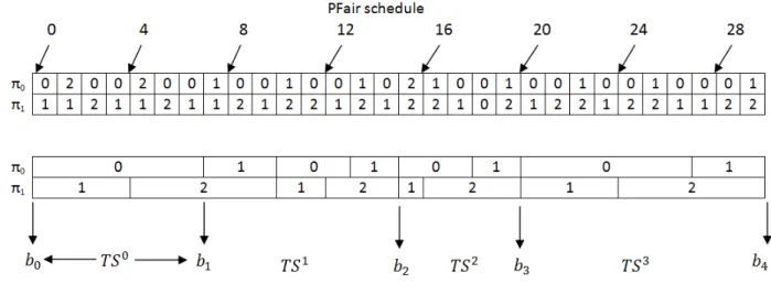
In Figure 5.2 task τ0 requires 4 preemptions using BFair instead of 11 using PFair. Which

shows that it is possible to deduct the number of preemptions and migrations of corresponding tasks by only regrouping all the time units of the same task within a time sliceT Sk,

Using empirical evaluation Zhu et al. [2003] showed that BF is also an optimal algorithm for periodic tasksets with implicit deadlines. And also the number of scheduling points is 25-50% of the number for a PD algorithm.

Another boundary fair scheduling algorithm PL was proposed by Kim and Cho [2011]. It was designed for a set of synchronous periodic tasks. PL stands for pseudo laxity. The PL algorithm uses prioritization rules of PD2 to distribute the optimal time units and rather than utilizing McNaughton’s wrap around algorithm, utilizes LLF (Least Laxity First) algorithm to generate the schedule within each time slices. The PL algorithm was also proven optimal for synchronous periodic tasks with implicit deadlines by Kim and Cho [2011].

The BF2 scheduling algorithm:

The scheduling algorithm BF2is proposed by Nelissen et al. [2014]. It is based on BFair schedul-ing algorithm. But, there is a significant difference between BF algorithm proposed by Zhu et al.

5 Related Work on Real-time Scheduling Techniques

Figure 5.2: Pfair and BFair schedules of three tasks τ0, τ1 and τ2 , where number of processors ism = 2. The periods are T0 = 15, T1 = 10, T2 = 30,and the worst-case execution times areC0 = 10, C1= 7, C2= 19,[Nelissen et al., 2014]

[2003] and BF2. The algorithm BF is optimal only for periodic tasks while achieving full system utilization, but cannot handle sporadic tasks because of their inherent irregular and unpre-dictable job release pattern. By the same token, BF2 is an optimal algorithm for sporadic tasks. Nelissen et al. [2014] also showed that their proposed algorithm BF2 outperforms the state-of-the-art optimal scheduler PD2 by benefiting from less scheduling overhead.

The PD2∗ scheduling algorithm:

Previously we described that PD2 defines the group deadlineGD(τi,j) as light tasks (i.e., tasks with Ui <0.5) and heavy tasks (i.e., tasks withUi >0.5). In particular, the group deadline is defined in PD2∗ not in the same way as it is in PD2. In PD2∗for light tasksGD(τi,j) is always 0

and for heavy tasks defined by the earliest time instant after or at the pseudo-deadlinepd(τi,j) following a succession of pseudo-deadlines separated by only one time unit [Nelissen et al., 2014]. Therefore, group deadlines for all the tasks are identical. This new algorithm PD2∗ is proposed by Nelissen et al. [2014]. It is a slight variation of PD2.

Thegeneralized group deadline is denoted byGD∗(τi,j) and defined as follows [Nelissen et al., 2014]: The generalized group deadline GD∗(τi,j) of any subtaskτi,j of a taskτi, is the earliest time t, where t ≥ pd(τi,j), such that either (t = pd(τi,k)∧bτi,k = 0) or (t = pd(τi,k) + 1∧ (pd(τi,k+1)−pd(τi,k))≥2) for a subtask τi,k ofτi such thatk≥j [Nelissen et al., 2014].

And the prioritization rules are given by the same authors are as follows:

Prioritization Rule 5.2.3. A subtaskτi,j has a higher priority than a subtask τk,l under PD2∗ iff:

1. pd(τi,j)< pd(τk,l)

2. pd(τi,j) =pd(τk,l)∧b(τi,j)> b(τk,l)

3. pd(τi,j) =pd(τk,l)∧b(τi,j) =b(τk,l) = 1∧GD∗(τi,j)> GD∗(τk,l)

5.3 Summary

Though this proposed algorithm is a modified version of PD2, the authors [Nelissen et al., 2014] proved the optimality of PD2∗for sporadic task sets as well as intra-sporadic and dynamic tasksets under a PFair or ERFair policy.

The LLREF scheduling algorithm:

LLREF is introduced by Cho et al. [2006]. It is based on fluid scheduling model employing L-T plane abstraction, it is also an optimal algorithm for periodic tasksets with implicit deadlines. In LLREF, scheduling timeline is separated into sections by normal scheduling events. At the beginning of each start section, selection ofm task is done for execution based on largest local remaining execution time first (LLREF) [Davis and Burns, 2011]. The local remaining execution time decreases during task execution in the section.

The LLREF approach was extended by Funaoka et al. [2008] as a work-conserving algorithm by distributing the unused processing time among the tasks and combining the processing time after completion of a task earlier than expected. Funaoka et al. [2008] showed that with this approach the resultant preemption is significantly less than in the case of LLREF when taskset utilization is below 100%.

Another extension of LLREF was done by Funk [2010] and is known as LRE-TL. Funk [2010] noticed that a task selection is not necessary for the execution based on the largest local remain-ing execution time within each execution. Funk [2010] also represented that LRE-TL algorithm could be applicable to sporadic tasksets and also proved the optimality with utilization bound of 100% for sporadic tasksets with implicit deadlines [Davis and Burns, 2011].

The EDZL scheduling algorithm:

EDZL stands for Earliest Deadline until Zero Laxity. It was introduced by Lee [1994]. With this algorithm Lee [1994] showed that it dominates global EDF scheduling. Lee [1994] also presented that for two processing cores EDZL is suboptimal. Here the meaning of suboptimal

is defined by the notion that EDZL can “schedule any feasible set of ready tasks” [Davis and Burns, 2011].

A variant of EDZL, introduced by Kato and Yamasaki [2008] is Earliest Deadline until Critical Laxity. This algorithm increases the job priority based on critical laxity at release time or completion time of a job. This technique reduces the minimum number of context switches to two per job which is achieved by slightly inferior schedulability compared to EDZL [Davis and Burns, 2011].

5.3

Summary

A performance measurement of partitioned, clustered, and global scheduling approaches was conducted by Brandenburg et al. [2008] using EDF and Pfair algorithms on LITMUSRT _test-bed

on the Sun UltraSPRAC Niagra multi-core platform with 32 logical processors (four hardware threads running on each of eight CPUs). It was observed in their experiment that in the context of overhead, staggered Pfair performed much better that pure Pfair, in other words, pure Pfair performed very poorly. Another poor performance was found for Global EDF scheduling algorithm due to the overhead caused by manipulation of a lengthy global queue accessible to all processors. For hard real-time tasksets, Partitioned EDF works best except when the tasks had high individual utilization. In contrast to that, staggered Pfair was the best.

Another performance measurement experiment was conducted by Nelissen et al. [2014]. They explored fair scheduling approaches using pure Pfair, i.e., PD2, partially Pfair BF2 algorithms

5 Related Work on Real-time Scheduling Techniques

on Linux kernel version 2.6.34 on the multi-core platform of Lenovo ThinkStation having two Xeon E5405 Intel chips, where each chip has four cores of 2 GHz. Though, their machine was composed of eight identical cores, only six of them were used to run the real-time tasks and the rest of the CPUs were utilized for debugging and monitoring purposes. BF2 was implemented using work conserving technique and PD2 was implemented in its early-release version. It was the best performing implementation of PD2 according to Anderson and Srinivasan [2000]. It is worth mentioning that the ERfair version of PD2 is also work conserving. It was observed in their experiment that for BF2 the number of preemptions, migrations, and scheduling points barely depends on the system time units when these values increase linearly with time resolution of the system running PD2. Also confirming the same conclusion of Brandenburg et al. [2008], they showed that in their experiment BF2 performed better than PD2 in terms of overhead. In their report, they also mentioned that in terms of preemption and migration the results of PD2∗ would be similar to PD2. On the other hand, its scheduling overhead would be worse [Nelissen et al., 2014].

In this thesis work, performance measurement is done using PD2∗ proposed by Nelissen et al. [2014] as a new slight variation of PD2 already described in this chapter.

6.

Related Work on Real-time Scheduling

Test-beds

A drastic expansion of interest in real-time task scheduling for multi-core systems inevitably led to increased interest in multi-core architectures. In recent time, a significant amount of efforts has been devoted to this field by the academic community, focusing extensively on theoretical issues [Dellinger et al., 2012].

For analyzing temporal constraints of tasks in a real-time application/system a number of tools have been developed which include graphical editors and frameworks providing classical real-time scheduling/feasibility algorithms/tests, both in commercial and free distribution, e.g. STORM, Harmless (Hardware Architecture Modeling Language for Embedded Software Simulation) and YARTISS based on Java for comparing user-customized algorithms. The latter can also simulate tasksets considering energy consumption as a scheduling parameter in the same manner as Worst Case Execution Time (WCET). Another tool Cheddar is based on Ada, it includes a graphical editor made using GtkAda. Cheddar is compatible with Solaris, Linux, and win32 systems and GNAT/GtkAda supported platforms. It also supports AADL, STOOD, TOPCASED plug-ins. Though research of algorithms is fundamental for the advances in multiprocessor real-time scheduling, in particular on platforms with a large number of cores, the effects of system overhead on scalability of existing schedulers are not explicit [Dellinger et al., 2012]. In other words, a simulation test-bed has to be real-time by itself, in the context of both logical and first of all physical functionality.

Also worth mentioning is the development of an optimal multiprocessor Real-Time Operating System (RTOS), while test-bed specific trade-offs of computational efficiency of the processing architecture should also be evaluated. That includes the architectures for general purpose micro-processors and powerful DSP kernels up to optimally tailored Application Specific Instruction set Processors (ASIPs).

In general, task scheduling is implemented in the operating system kernel. Therefore, a variety of kernel/kernel-level components have been developed as testing platforms of real-time scheduling on the Linux kernel as this approach has a few definite advantages such as the availability of libraries, software development tools and software packages for a wide variety of purposes.

For enabling implementation for small systems, POSIX1.3 is defined as RT-POSIX[Buttazzo, 2004] [iee, 2004][MARTE, 2011].

1. PSE51: Minimum Real-time System Profile 2. PSE52: Real-time Controller Profile

3. PSE53: Dedicated Real-time System Profile 4. PSE54: Multi-purpose Real-Time System Profile

The interest of using Linux as underlying operating system for embedded applications has also been actively pursued by the industry. This selection also provides the ability of hosting both real-time and best-effort tasks on the same CPU [Betz et al., 2009]. Moreover, some real-time extensions of Linux provided competitive results against commercial ones[Barbalace et al., 2008] [RTAI, 2014][Xenomai, 2014]. Therefore, we will avoid detailed discussions about commercial real-time systems with simulation features such as VxWORKS, OSE, ONX NEUTRIO.

6 Related Work on Real-time Scheduling Test-beds

6.1

Linux-kernel

Kernel is a program which constitutes the core of the operating system, acquiring the complete control over the operating system. A well known kernel for a Unix-like operating system is Linux kernel released under GNU GPL2 license. Linux kernels can be categorized considering their architecture.

• Monolithic kernel: A very large number of Linux variants use the monolithic kernel. Com-pared to others it is large, and each of the kernel layers is unified with the whole kernel program. In support of the current process, it runs in Kernel Mode [Bovet and Cesati, 2001]. In a monolithic kernel architecture, the entire operating system is in the kernel space and executing entirely in supervisor mode for all process scheduling subsystem memory management, IPC, virtual files, network. That directly opposes a microkernel architecture. • Microkernel: Compared to the monolithic kernel, microkernel based operating systems require a tiny set of functions from the kernel which includes a few synchronization prim-itives, a scheduler, and an IPC mechanism [Bovet and Cesati, 2001]. A kernel module is such an object file which can be linked and unlinked to the kernel at runtime. To utilize the advantage of microkernels, Linux kernel offers modularized approach. Therefore, relevant data structures can be accessible by well defined interfaces [Bovet and Cesati, 2001]. • Hybrid kernel: A hybrid kernel architecture is built with flavour of both of microkernel

and monolithic kernel architectures. The main goal behind this combined approach is to provide a kernel structure as microkernel in a monolithic kernel implementation method-ology.

Almost all the operating services as basic IPC, virtual memory, scheduling techniques including application IPC and device drivers are in kernel space, which avoids performance overhead for context switching and message passing between the kernel mode and user mode. From the architectural point of view, integration of application IPC and device drivers are different in hybrid kernel from the others.

6.2

Kernel Preemption

A kernel is considered to be a preemptive kernel if process switch is possible in Kernel Mode. In the case of non-preemptive process switching, the switch is called planned process switch. In contrast, in case of preemptive switching the switch is called forced process switch. The main feature of a preemptive kernel is the process switching in Kernel Mode. This can also be seen when in the middle of a kernel function a running process in Kernel Mode can be preempted and replaced by another one.[Bovet and Cesati, 2001]

Apart from supporting a variety of kernels, the SMP offers features which are significantly relevant for designing RTOS on multi-core architectures. From version 2.6 Linux kernel supports SMP with different memory models including NUMA.

Moreover, the first appearance of multiprocessor RTOS implementation in a hard real-time form for Linux is found during the 1990s and is also known as dual kernel [Lehrbaum and Rick, 2000][Bicer et al., 2006]. Generally multiprocessor RTOSs insert a thin layer between the hardware and general purpose operating system for taking over the interrupts and also have