Balanced Traffic Routing: Design, Implementation, and
Evaluation
Ruilin Liu* , Hongzhang Liu* , Daehan Kwak* , Yong Xiang†, Cristian Borcea‡, Badri Nath* , Liviu Iftode*
*Dept. of Computer Science, Rutgers University, Piscataway, NJ 08854, USA {rl475, antony26, kwakno1, badri, iftode}@cs.rutgers.edu
†Dept. of Computer Science and Technology, Tsinghua University, Beijing, 10084, China
‡Dept. of Computer Science, New Jersey Institute of Technology, Newark, NJ 07102, USA
Abstract
Navigators based on real-time traffic conditions achieve suboptimal results since, in face of congestion, they greedily shift drivers to currently light-traffic roads and cause new traffic jams. This article presents Themis, a participatory system navigating driver-s in a balanced way. By analyzing time-driver-stamped podriver-sition reportdriver-s and route decidriver-siondriver-s collected from the Themis mobile app, the Themis server estimates both the current traffic rhythm and the future traffic distribution. According to the estimated travel time and a popularity score computed for each route, Themis coordinates the traffic between alternative routes and proactively alleviates congestion. Themis has been implement-ed and its performance has been evaluatimplement-ed in both a synthetic experiment using real data from over 26,000 taxis and a field study. Results from both experiments demon-strate that Themis reduces traffic congestion and average travel time at various traffic densities and system penetration rates.
Keywords: Cooperative Routing, Participatory Sensing, Mobile Application, ITS.
1. INTRODUCTION
The widespread deployment of mobile devices has lead to many mobile apps for traffic navigation. According to Ericsson ConsumerLab, 29% of smartphone users in the U.S. used Google Maps or other smartphone navigation apps during morning commute in 2011 [1], and this number has increased since then. Given the similar number of dedicated navigation devices [2], the penetration rate of dynamic navigation devices or apps is now considerable.
Modern drivers equipped with GPS-enabled devices not only use the traffic infor-mation but also act as traffic inforinfor-mation providers. Popular navigation apps, such as Google Maps [3] and Waze [4], have been prevalently applying the location and event reports from smartphone users to compute the estimated time of arrival (ETA) of the
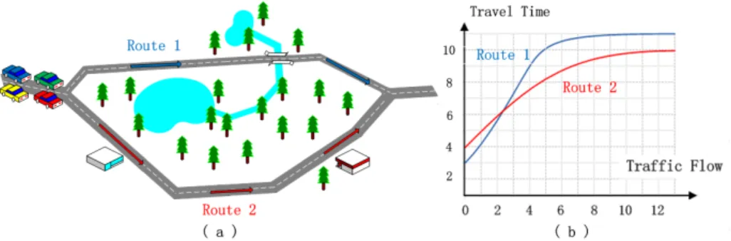
Figure 1: Four cars are about to choose route 1 or route 2 to go from left to right in (a). Due to no traffic, the latest estimated travel times are three minutes and four minutes for two alternatives, respectively. However, if each car greedily takes route 1, given the travel-delay model of the two routes in (b), the actual travel time for route 1 will be nine minutes, three times of the estimated value.
alternative routes. Driving experience and fuel consumption are also shared in novel systems [5, 6] to help users select among several route choices.
In spite of the progress, one strategic problem with the current navigators still ex-ists: They greedily route drivers to the fastest path based on the periodically updated traffic conditions. The high penetration of these navigators potentially leads to the Braess’s paradox [7] caused by the coupled route choices. For instance, in Figure 1, greedy routing leads all of the four vehicles to the same route. Since vehicles need time to reach the bottleneck of the planned route, subsequent drivers may have already made their decisions before the influence of previously routed cars is reflected in the traffic conditions. The coupled “best” route choices actually lead the drivers to traffic congestion and longer travel time instead of saving their travel time. Note that rerout-ing is not expected to solve the problem, either because reroutrerout-ing is too late or because it leads all traffic to new “best” routes and causes new jams. Actually, agent based sim-ulation has demonstrated that the average travel time increases when half of the drivers follow the dynamic fastest path based on retime traffic [8]. Roughgarden [9] has al-so elaborated on the suboptimal global situation caused by the greedy routing without coordination.
A few routing algorithms have been proposed to overcome the drawback of greedy routing [10, 11, 12, 13, 14, 15]. These algorithms, employingcooperative routing, plan routes based on anticipated traffic volume (ATV) and corresponding predicted travel time (PTT) by assuming previously routed cars follow their suggested routes. For example, in Figure 1, two cars may anticipate the future congestion on route 1 and take route 2 instead, even if route 2 has longer ETA based on the real-time traffic. In our prior work [16], we also presented a cooperative routing algorithm, EBkSP, to route traffic based on both ETA and the popularity of the candidate routes.
Despite plenty of algorithmic studies, there are still no practical cooperative routing services deployed in real life. We believe this is due to two types of challenges. First, there are a number of practical aspects that have to be solved when building a cooper-ative routing service: (1) What routing algorithm can be chosen and how can it work at low penetration rates? (2) How to estimate the average speed accurately? (3) How
to predict the future traffic flow? (4) Most importantly, how to incorporate the above components in one system to provide cooperative routing services? Second, the service has to be evaluated in a meaningful way before deployment: (1) How to realistically evaluate the system without large-scale real-life experiments? (2) How to evaluate the performance under different penetration rates? This article addresses both aspects.
In this article, we present a participatory cooperative navigation system, Themis, which utilizes the data collected from road vehicles, such as location samples and route choice decisions, to estimate the traffic speed as well as the future traffic flow at road segment level. By learning and combining the multi-dimensional traffic information, Themis applies a cooperative routing algorithm to route the participant drivers to routes that are good for both the drivers and the traffic ecosystem to proactively alleviate congestion.
Furthermore, we present a method to investigate how the performance of a partici-patory navigation system scales at different penetration rates by meaningfully expand-ing the real data collected from probe vehicles. We apply the method to the trajectory data from over 26,000 taxis and demonstrate that Themis outperforms greedy naviga-tion systems. We find that the benefits of Themis emerge even if the penetranaviga-tion rate is as low as 7%.
Finally, we prototype Themis as a vehicular routing server and an Android smart-phone app. The prototype system is validated in a field study with 16 cars and it illustrates Themis’s benefits in terms of traffic distribution and travel time reduction in real world when the penetration rate is almost 100%.
The remainder of the article is structured as follows: Section 2 reviews the re-lated work. Section 3 describes the Themis architecture and elaborates on the algo-rithms used by each component. Section 4 covers the implementation details of our Themis prototype system. The evaluation using city-scale synthetic experiments and neighborhood-scale field experiments are presented in Sections 5 and 6, respectively. Section 7 discusses the lessons learned and the future work. The article concludes in Section 8.
2. RELATED WORK
Several algorithms were designed to solve the cooperative routing problem, and they can be divided into three categories.
The first category of algorithms focus on user equilibrium [17], which computes the PTT of road segments and plans the fastest path for a driver based on PTT. Since PTTs increase with ATVs which include the previously routed cars, the algorithms of this category automatically route subsequent traffic to the alternatives if previously routed traffic have made current fastest path (i.e., fastest path based on real-time traffic) suboptimal. Yamashita et al. [10] used Greenshield’s model [18] to relate PTT to ATV and designed the Passage Weight heuristic to generate the contribution of each planned path toward ATV. The work in [11] used a similar model to relate PTT and ATV except that it assumed the traffic volume to be stochastic and determined by both historical traffic and previously assigned traffic. In [14], the authors proposed to compute a few alternative routes based on real-time traffic and then route the car to the path with the shortest PTT based on encounter prediction.
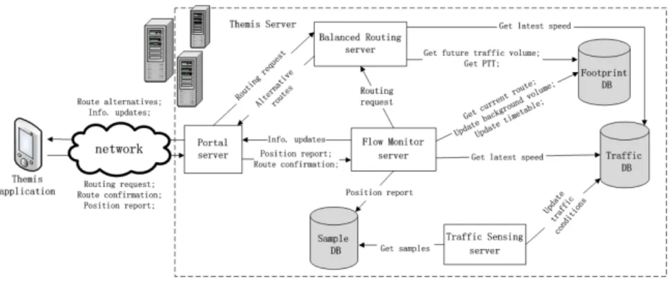
Figure 2: Themis System Architecture
Other studies aim to route the traffic to achieve system optimum of the transporta-tion network, which does not necessarily minimize the individual driver’s travel time but minimizes the average travel time of a group of users, e.g., all the drivers in a city or the users of a certain navigation system. The routing algorithms based on system optimum are also called social navigation [15]. Bosch et al. [15] proposed to handle a routing request by searching a path minimizing the total PTT of all previously assigned drivers. Lim et al. [12] proposed to compute a few route candidates based on real-time traffic and investigate the mutual timing influence of users’ route choices based on the BPR flow-delay model [19]. This work assigns a group of drivers to the combination of paths that optimize the total travel time, and the algorithm was evaluated using taxi trajectory data from Singapore [20].
Finally, Pan et al. proposed several heuristics to plan or to choose from the first-k shortest paths (KSPs) based on previously assigned traffic [16]. The basic workflow of these approaches is similar to aforementioned two categories. However, the criteria used to compute or choose from KSPs in these approaches are not precisely computed PTT but some heuristic functions. For example, the EBkSP algorithm computes the KSPs according to real-time traffic and assigns the traffic to the least popular route among KSPs to balanced the traffic volume distribution. The popularity heuristic is de-fined based on both current traffic conditions and previously routed traffic (i.e., ATV). Simulation result shows that the heuristic methods achieve substantial travel time re-duction with very limited computation resources.
In this article, we address the challenges of implementing these algorithms in real life. We present a participatory system, using up-to-present data collected from cars to determine the traffic conditions, based on which cooperative routing algorithms make decisions (i.e., real-time traffic and PTT or ATV). Compared with the taxi data evalua-tion in [20], our synthetic evaluaevalua-tion method investigates the performance of coopera-tive navigation at different penetration rates by meaningfully expanding the trajectory data. In addition, we also include the real world evaluation results from field studies.
3. PARTICIPATORY NAVIGATION SYSTEM
The Themis app is assumed to be installed in a mobile device, which is equipped with GPS and wireless communication such as DSRC or cellular to connect with the Themis server. The route computation is carried out at the Themis server using a coop-erative routing algorithm. While the route suggestions are retrieved by the Themis app to provide users with turn-by-turn directions, the app also uploads route confirmations and time-stamped positions to help deal with subsequent navigation requests.
3.1. System Architecture
As illustrated in Figure 2, Themis consists of five executable entities: the Themis app on mobile devices, the Portal server, the Traffic Sensing server, the Flow Monitor server, and the Cooperative Routing server. While logically centralized, each server can be implemented in a distributed fashion to provide scalability. The Themis app allows the drivers to select from suggested routes, presents turn-by-turn driving directions, and uploads time-stamped position reports as well as the route selection decisions. The Portal server ensures the interaction between the Themis server and the Themis app and meanwhile performs request dispatching and load balancing. The Traffic Sens-ing server estimates the travel time at road segment level. The Flow Monitor server supervises cars’ movement along its selected route, triggers rerouting if needed, and estimates the future traffic that is scheduled to travel through each road segment. In addition, it is responsible to update the traffic information (e.g., ETA) for users. The Cooperative Routing server computes the route candidate(s) based on real-time speed, PTT, and ATV.
The information used by the Cooperative Routing server is stored in two databases. The Traffic database stores the static road map, the traffic-delay model, and the latest estimated travel time of each road segment; it is updated by the Traffic Sensing server. The Footprint database maintains the routes being taken by drivers and their status, such as the timetables containing the ETA to each road segment included in the confirmed routes. It also stores the short-term predictions of the traffic flow on each road segment (i.e., how many cars will go through a road segment in the future) based on the routes being taken and the latest traffic conditions. The Footprint database is updated by the Flow Monitor server. The Sample database is only used to cache the position reports.
Navigation Process.When a user issues a new navigation request, the Themis app contacts the Portal server with the origin-destination information. The Portal server for-wards the routing request to the Cooperative Routing server, where route candidates are calculated using data from the Traffic and Footprint databases. The routing results are returned to the Themis app by the Portal server to generate alternative route previews. The user chooses one of the alternatives, and the Themis app translates the selected route into turn-by-turn directions. A confirmation of the selected route is meanwhile sent back to the Flow Monitor server to update the Footprint database.
Position Report Process. During regular driving, the Themis app periodically re-ports time-stamped positions (also called samples) to the Portal server, which are then sent to the Flow Monitor server. If the position is successfully matched to the previ-ously confirmed route, the Flow Monitor server will provide the user with the latest ETA and earned route score (see Section 3.4) and update the timetable belonging to
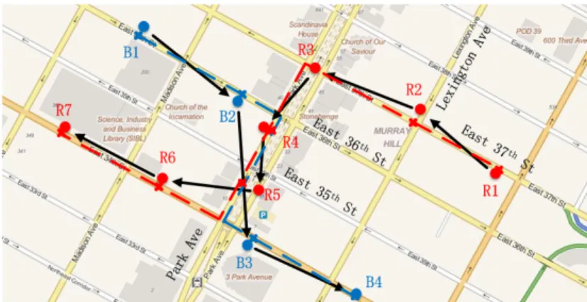
Figure 3: An example of participatory traffic sensing. Red and blue dots represent the trajectories from two different cars in the same interval. Their movement directions are illustrated using arrows. After the map matching process, the samples in each trajectory are matched to points along the roads shown with crosses. Meanwhile, the inferred episode routes that connect the matched points (shown in dash lines) are used for travel time allocation and aggregation.
this route in the Footprint database; otherwise, a detour is detected and the Flow Mon-itor server will end the current confirmed route and issue a new routing request to the Cooperative Routing server. Note that, no matter whether the route matching process is successful or not, each position report handled by the Flow Monitor server will then be stored in the Sample database, from which the Traffic Sensing server retrieves samples to estimate the travel time of each road segment periodically.
3.2. Participatory Traffic Sensing
After collecting and preprocessing the position samples from multiple cars during an interval, the Traffic Sensing server takes the following steps to estimate the travel time on each road segment.
3.2.1. Map Matching
During the map matching process, samples are matched to the road map (i.e., to the most likely position on road segments), and the possible episode routes (i.e., partial routes) linking consecutive samples from each car are also inferred. Figure 3 shows how the episode routes are constructed.
Themis map matching is based on the Hidden Markov Map Matching (HMMM) method in [21], which considers both the distance to nearby roads and the context of each sample. For example, although sample R2 in Figure 3 is closer to Lexington Ave, it should be matched to East 37th St because it is unlikely for a driver to travel from R1 to R3 through Lexington Ave.
In [21], the context information used to compute the transition probability in HM-MM is the length of the episode routes connecting adjacent samples. Themis enhances it by defining the transition possibility based on Weighted Route Length (WRL). The motivation for this change is the observation that people tend to take main roads in-stead of lower-level (i.e., smaller) roads even if the length of low-level roads is shorter.
Supposepiis the i-th possible episode route between two matching samples, then: W RL(pi) =
X
e∈pi
lene∗weightl(e), (1)
whereleneis the length of the road segmenteandweightl(e)is the weight associated
with the level of the road segmente. The HMMM method essentially computes the probability of several episode route candidates, each of which is a function using the weights as its parameters. Therefore, theweightof each road level can be learned from real data (i.e., training data). In our case, we set the objective function as maximizing the sum of the probability differences between the ground truth path and all the other paths. Then, we determine the value ofweightusing over 15,000 manually matched samples.
3.2.2. Travel Time Allocation and Aggregation
The episode routes inferred through the map matching process may consist of mul-tiple road segments and even partial road segments. Travel time allocation process divides the travel time observed on an episode route to the road segments covered by this route using the estimated travel time in the previous interval. For example, the trav-el time from B2 to B3 in Figure 3 is distributed to the two fully covered road segments and the two partially covered road segments.
Given an episode routepi and the travel time observationτi, the travel time
allo-cation process computes a travel time estimation for each road segment covered bypi,
defined asRpi(ei,1, ei,2, ..., ei,n). For a road segmentei,jpartially covered bypi, we
defineρi,j as the fraction of covered length out of the total length ofei,j. We denote
the travel time estimation on road segmentei,jin previous interval (i.e., intervaln−1)
as¯tni,j−1. The travel time on road segmentei,j estimated from the episode routepi,
denoted asτn
i,j, is computed as follows: τi,jn = ¯ tni,j−1 P ei,k∈Rpi ρi,k∗¯tni,k−1 ∗τi (2)
Supposep(p1, p2, ..., pn)is the collection of episode routes covering a specific road
segment within intervaln. The aggregation process utilizes the time estimations for this segment drawn from eachpi ∈pand aggregates them into one travel time expectation
value. As shown in Figure 3, by allocating the travel time of episode route (R3, R4), episode route (R4, R5), and episode route (B2, B3), respectively, we have three travel time estimations for the road segment from East 36th St to East 35th St on Park Av. The estimations are aggregated to gett¯n
e, the travel time estimation of edgeein intervaln:
¯ tne = P pi∈p,ei,j=e τn i,j∗ρi,j/τi P pi∈p,ei,j=e ρi,j/τi (3)
The aggregation process smooths the influence of the non-traffic factors, such as the driving style. Equation (3) calculates the weighted average value of individual estimations, which biases the estimation in favor of the episode routes with longer coverage and the episode routes with higher sampling rates.
3.3. Flow Monitor
The basic function of the Flow Monitor server is to estimate ATVs on road seg-ments such that PTTs could be inferred based on given traffic-delay models. Since the penetration rate of Themis is not expected to be 100%, the ATV includes both the controlled traffic and the unexposed background traffic.
The controlled traffic represents the cars that use Themis to plan paths and navigate to destinations. This part of traffic can be determined easily. Once a route is confirmed by the Themis app, the Flow Monitor server translates the planned path into a timetable, in which the ETA to each road segment in the path is sequentially estimated starting from the current location using the latest travel time estimations. The timetable is updated when a new route confirmation or location report is received. Based on the timetable, the controlled traffic volume can be estimated given a road segment and a time-stamp.
The method used to estimate the background traffic in Themis is based on [22], which proposed to extrapolate unexposed traffic volume based on some naturally dis-tributed probes. In Themis system, we use the controlled traffic as the probes and dynamically estimate the ratio of the controlled traffic volume to the background traf-fic volume on each road segment based on the known ratios from baseline road seg-ments and the similarity between the road segseg-ments. This algorithm has been proven to have good performance given accurately estimated real-time speed and controlled traffic volume generated by a large number of natural probes. In Themis, the estima-tion of real-time speed is discussed in Secestima-tion 3.2. However, we cannot directly use the controlled traffic volume computed in the previous paragraph to infer the back-ground traffic because the paths of controlled traffic are not “natural” (as expected by the method in [22]) but influenced by the cooperative routing system. Currently, we assume the natural path to be the fastest path and estimate the natural traffic volume by assuming cars move using the latest estimated speed along the natural path. Although there may be exceptions when users would not take the fastest path in the absence of Themis, we leave more accurate natural path inference for future work.
3.4. Cooperative Routing Algorithm
Two routing algorithms are implemented in the Themis routing server, the Dijkstra fastest path based on the real-time travel time estimation, and a balanced routing algo-rithm. The basic workflow of the balanced routing algorithm is presented in Alg. 1. Themis first computes the alternative routes based on real-time traffic, and then exe-cutes a popularity scoring algorithm to evaluate the popularity of each possible route.
For the computation of alternatives (i.e., KSPs), we choose the Iterative Penalty Method (IPM) [23] as simulation results showed that IPM could provide dissimilar KSPs with small computational cost. We define the similarity between two paths as the ratio of the length of the overlapped road segments out of the total length of the shorter path. By setting a threshold of similarity, IPM terminates either when enough dissimilar paths have been computed or when there have been too many iterations.
After computing the route alternatives, Themis associates a score with each alter-native, which reflects the popularity of that route. The score is inversely related to the route popularity. Given that traffic conditions are periodically updated, routing cars to
Algorithm 1Balanced Routing Algorithm
Input: origin, destination, traffic database, footprint database, similarity threshold, number of paths,: max iteration
Output: alternative routes with scores
1: π=∅; {initialize the set of alternative routes}
2: π= get_dissimilar_KSPs (origin, destination, traffic database, similarity threshold, number of paths,);
3: for all πi∈π do
4: πi.score = compute_score(πi, traffic database, footprint database);
5: end for
a routeπiresults in lower score for any route that has overlapping road segments with πi in a traffic condition update interval. Consequently, taking a route with a higher
score does not create congestion on this route, and this decision is expected to alleviate congestion elsewhere. Themis leaves the route selection decision to the user, who will attempt to find a balance between the estimated travel time and the score of each alter-native. By selecting an alternative with a higher score and with a good, but perhaps not the best ETA, a user will contribute to the global traffic ecosystem (i.e., the system’s state will move closer to the system optimum).
To compute the popularity score, we applied the following equation based on the popularity computed in EBkSP [16]. The score of an alternative routeπiis defined as:
scoreπi =
ET Aavg pop(πi)
, (4)
whereET Aavg is the average ETA for all the alternative routes and pop(πi) is the
popularity of routeπi. pop(πi)is determined by both the ETA of the route and ATV
that is scheduled to fully or partially travel through routeπi. IncludingET Aavg in
the equation does not influence the route choice. We add this term only to scale the magnitude of the scores.
4. PROTOTYPING
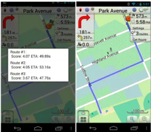
We implemented the Themis app on Galaxy Nexus (Android 4.3) based on an open-source GPS navigator, OsmAnd [24]. The Themis app is implemented as a plugin, together with a customized map layer, such that it can easily be switched on or off. We inherit the interfaces of turn-by-turn driving assistance provided by OsmAnd and move the route calculation to the Themis server. The user interface of Themis is shown in Figure 4. Themis computes three alternative routes based on real-time traffic conditions and associates each route candidate with the popularity score and its ETA. During the navigation process, the app listens to position change events and routing requests from the user. The former triggers a potentially new position update request, and the latter directly starts generating a routing request. These requests are sent to and replied by the Portal server via a JSON Interface.
Figure 4: Themis application interface. The left screenshot shows three possible routes ordered by their scores and ETAs. After choosing one route from the three alternatives, a user enters the navigation mode (right screenshot), which provides turn-by-turn driving directions. During the navigation mode, the upper left part of the screen displays the driving directions for the next two steps. The score that a user has earned so far for taking the current route is shown below the driving directions. The labels in the upper right part show the distance to the destination, estimated arrival time, and other route choices.
The Themis server is physically built on a Dell PowerEdge T110 server equipped with Intel Xeon E3-1230 v2 3.30GHz Quad Core processor, 4×8GB 1600MHz DIMM-s, and 2T 7200RPM SATA 3Gbps hard drive. The Portal server, Cooperative Routing server, and Flow Monitor server are implemented using PHP scripts. The Cooperative Routing server and Flow Monitor server expose their core functions to the Portal serv-er. When a route confirmation, routing request, or location report request arrives, the Portal server directly calls the corresponding functions in either the Cooperative Rout-ing server or the Flow Monitor server to handle the request. The Traffic SensRout-ing server is implemented as three separate java programs (i.e., map matching, travel time allo-cation, and travel time aggregation). As the location reports are stored in the Sample DB, the Traffic Sensing server just takes the records from the database for processing. For scalibility, in each interval, the server launches four instances for map matching and travel time allocation; for the aggregation process, one instance is enough in our experiments due to the low complexity of the task.
The implementation of the Themis server combines several open-source software packages to provide cooperative routing. OpenStreetMap (OSM) [25] is imported into PostgreSQL[26] database as the source of static map data by using osm2pgrouting [27]. The traffic information estimations are also stored in the PostgreSQL database as properties of each road segment. The two algorithms presented in Section 3.4 are implemented based on the open-source routing library pgRouting [28].
5. SYNTHETIC EVALUATION
This section analyzes the performances of Themis in synthetic scenarios modeling a city-scale deployment in Beijing using trajectory data from 26,000 taxis. Specifically, this experimental evaluation addresses the following questions:
1) How accurate is Themis’s participatory sensing in estimating the traffic charac-teristics?
2) How does balanced routing compare with greedy routing in terms of traffic dis-tribution and average travel time?
3) How do the traffic distribution and travel time vary with the system penetration rate and the total traffic amount?
The baseline routing algorithm in the evaluation is greedy routing (i.e., fastest route based on latest ETA) and for balanced routing, we assume that drivers choose the al-ternative route with the highest score.
5.1. Experimental Methodology 5.1.1. Dataset
We use GPS trajectories from a 26,000 fleet of taxis in Beijing during three consec-utive Tuesdays starting from April 6, 2010, which amount to approximately 58,000,000 valid data points. Each sample contains the taxi ID, the timestamp, the geo-location, and the passenger status (i.e., free or occupied). They are sampled at intervals between 30 seconds and five minutes. To derive the total traffic, we use two other datasets: the daily percentage of taxi traffic out of total traffic on 3981 main road segments, and the citywide half-hour variation of taxi traffic out of total traffic. By checking both the cov-ered area and the taxi penetration rate, we decided to carry out our experiment using the data in a rectangle area covering the Beijing second ring area, which is about 65 square kilometers. In this area, our taxi data account for almost 7% of the total traffic.
During the synthetic experiments, we imported the above datasets into the databas-es used by the Themis sever and procdatabas-essed them using our Themis service ddatabas-escribed in Section 4, including the Traffic Sensing server, the Flow Monitor server and the Coop-erative Routing server. As a result, even though with historical data, the Themis server is thoroughly evaluated with large amounts of real data.
5.1.2. Modeling Trips and Penetration Rates
The first problem we solved in the synthetic evaluation is how to extract routing requests from the dataset and manipulate them to get different penetration rates. First, we identify passenger-on-board (POB) trips. The time-stamped location where the passenger status of the taxi changes to POB is recognized as the origin of a POB trip. The time-stamped location where the POB status is reset to a different status is con-sidered as the destination. Since the number of POB trips is limited, especially during late-night hours, we also include non-passenger (NP) trips, which are those trips hap-pening between POB trips. We limit the max duration of NP trips to five minutes to avoid the influence of vacant wandering taxis. The routing requests generated in this way could be used to evaluate Themis when the penetration rate is no more than the original percentage of the taxis in traffic.
For the sensitivity analysis at higher penetration rates, we built a threefold and a sixfold routing request set. The threefold routing request set is generated by proposing each original routing request three times and adding a random in-between delay within five minutes. The sixfold routing request set is generated likewise. Therefore, the penetration rate can be increased to approximately 20% and 40%, respectively.
Note that the global penetration rate is carefully bounded by 40% such that, on any road segment, the traffic generated by the amplified routing request set does not exceed the total traffic estimated using the original routing request set (this will be presented in Section 5.1.3). Different penetration rates only change the proportion of the con-trolled traffic but do not influence any global traffic features such as traffic volumes and average speeds. The essence of amplifying the request set is that we extract some background traffic on consecutive road segments and use it to generate new trips based on real previous trips. Comparing to the methods that randomly choose the routing requests and expand them, our method preserves the traffic conditions implied in the taxi trajectories dataset. Therefore, it is a more persuasive setup to show the realistic influences of balanced routing in the targeted city. There are other alternatives to adjust the penetration rate such as modeling the traffic demand based on the original routing request set and then generating the amplified request set based on the traffic demand model. Due to the complexity of such methods, we leave them as future work. 5.1.3. Background Traffic Estimation
At each penetration rate, the background traffic volume equals to the original total traffic volume minus the controlled traffic determined by different routing request sets (origin, threefold, or sixfold) under the original traffic condition. Based on the method from [22] (also described in Section 3.3) and our taxi ratio statistical data, we can derive the background traffic volume if we know the movement of the controlled traffic on the road segment.
Given any routing request set with original routes, the movement of the controlled traffic can be simulated at the original average speed, which can be estimated by ap-plying our traffic sensing algorithm (Section 3.2) to the taxi trajectory dataset. After each 15-min interval, we directly estimate the average travel speed on a road segment if there are at least two taxi trajectories passing through the segment during the interval. For the road segments that do not have direct estimations, we derive the estimated av-erage speed using the speed of their joint road segments. As discussed in Section 5.1.2, the estimated speed when the penetration rate is 7% can also be used for the other two penetration rates (i.e., 20% and 40%). We call the speed estimated using participatory traffic sensing thesensed speed.
5.1.4. Learning the Traffic-Delay Model
If every car takes its original route, the average travel speed on each road segment would be the original sensed speed. However, to evaluate the travel time of the trips after rerouting, this original sensed speed is not useable as reroutings dramatically change the traffic distribution. Therefore, we use a traffic-delay model [19] to infer the travel time of a road segment based on the traffic volume on it during a given time interval, which is determined as described in Section 5.1.3. The speed derived based on
the traffic-delay model is called theinferred speed, with the inferred travel time derived from it. The function used for the traffic-delay model is:
te(fe) =Te0(1 +α( fe Ce ) β ) (5) T0
e is the free-flow speed (i.e., speed limit). Ceis the capacity of the road segmente
andfeis the average traffic volume. te(fe)is the inferred speed based on the traffic
volumefe.
Using a similar method as [20], we learn the parametersαandβ for 7,411 road segments from the total of 11,450 road segments. These segments were used because they have good direct travel time estimation. Fortunately, these models cover most main roads. During the evaluation, we only route traffic over road segments that have traffic-delay models such that we are able to measure travel time changes. For the comparison between the actual travel time of the original routes and the inferred travel time using the traffic-delay models, we also only use the routes fully covered by the traffic-delay models.
5.1.5. Traffic Movement Simulation
Given the route and the average speeds in each interval, we simply simulate the trip by assuming a car travels through each road segment included in the route using the average speed of the current interval. As we know the starting time of the trip, we can compute the starting time of each road segment step-by-step. When the time reaches a new interval, we use the average speeds for this new interval.
One difficult issue is how to simulate the rerouted trips. After rerouting, the move-ment simulation must be done using the speeds inferred based on the traffic-delay mod-el. However, the traffic-delay model needs the traffic volumes to derive speeds. This is a chicken-and-egg problem because the traffic volume is determined by the movement of the traffic within the 15-min interval. To solve it, we use an iterative method to com-pute the speeds within each interval. In the first iteration, we use the sensed speeds to simulate the traffic movement. This step will end with new inferred speeds on the road segments. In the next iteration, we used the inferred speeds from the first iteration to update the speeds in the same interval. The process goes on iteratively until no speed changes on any road segment. Fortunately, the process converges very quickly because small speed changes do not influence the traffic volume distribution significantly. 5.2. Evaluation of Travel Time Estimations
The accuracy of either the sensed speed or the inferred speed is evaluated by a comparison between the average ground truth trip travel time and the average simu-lated trip travel time based on the corresponding speed estimations. To get the sensed speed, we apply the participatory traffic sensing algorithm (Section 3.2) to our taxi tra-jectory dataset. For the inferred speed, we apply the method in Section 5.1.5 to the 7% penetration routing requests set based on the learned traffic-delay model.
In the evaluation, we choose 100 random trips from the original request set in each 15-minute interval from 1:00 to 13:00 on April 6, 2010. We choose this period as it contains both peak hours and low-traffic hours. In addition, the number of taxis in
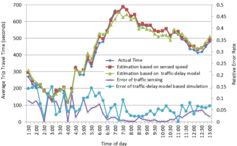
Figure 5: The accuracy of trip travel time estimation.
operation changes greatly during this period so that we can analyze the sensitivity of Themis participatory traffic sensing. At 4:00, only 7647 taxis (30% in our dataset) are running, while over 95% taxis operate between 9:00 and 9:30. For sensed speed evaluation, we use “leave-one-out” validation by not including the estimations from the car under evaluation into the aggregation step. However, the “leave-one-out” validation is not used for the inferred speed evaluation because the traffic-delay models are built using the data from three days, not specifically optimized for our evaluation set.
Figure 5 shows that the actual time and the simulated travel time computed based on sensed speed are closely matched, which means that the accuracy of our participatory sensing is high. During the period from 6:30 to 10:30, the relative error is less than 3%. The highest error comes during late-night hours when the participants are extremely sparse. However, even in this case, the relative error is below 12%. The results show that our participatory sensing algorithm has good accuracy and is robust to varying numbers of participants.
The travel time simulated using the inferred speed also matches the ground truth well. During the period from 6:30 to 13:00, the relative error is less than 10%. Similar to participatory sensing, the inferred speed also has a higher error rate during late night, which is less than 15%. These results prove that our traffic-delay model is acceptable.
In order to get the accurate evaluation of the balanced navigation system, we only carry out the following evaluation experiments between 6:30 and 13:00. Another rea-son to abandon the period between 1:00 and 6:30 is that during this period the traffic load is too low to generate traffic congestion.
5.3. Evaluation of Traffic Distribution
The average traffic volume is used as a global measure of congestion in the road network and is computed over all road segments that are traversed by at least one car. The higher the traffic volume, the less distributed the traffic; consequently, it is more likely to experience congestion in the network.
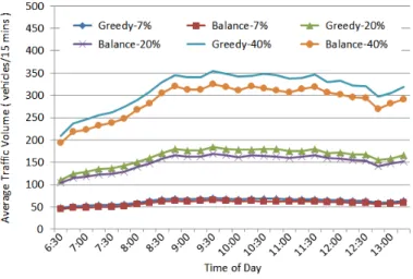
Figure 6: Traffic volume comparison at different penetration rates.
Figure 6 presents the comparison of the navigated traffic volume between two im-plemented routing algorithms in Themis (i.e., balanced routing and greedy routing, see Section 3.4) at different penetration rates. The balanced routing results in a lower traf-fic volume at each interval for each penetration rate. These results demonstrate that balanced routing distributes the traffic better than the greedy routing. Furthermore, the traffic volume is reduced more substantially for higher penetration rates. We al-so observe that, during the experimental period, the relative traffic volume reduction is steady at each penetration rate regardless of congestion levels. Another interesting finding is that the relative traffic volume reduction tends to increase more slowly as the penetration rate increases. This implies that, as the penetration rate rises above a cer-tain threshold, the balanced routing’s function to reduce global traffic congestion will linearly increase with the penetration rate.
5.4. Evaluation of Trip Travel Time
One danger of the balanced routing algorithm used in Themis system is that it could lead to longer trips when distributing traffic to unpopular routes. We define two criteria to compare the performances of balanced routing and greedy routing in terms of trip travel time in each 15 minutes interval:
F R=N umber(A
0s travel time < B0s travel time)
N umber(all the routing requests) (6)
RT T R= B
0s travel time−A0s travel time
B0s travel time (7)
Faster Rate (FR) reflects the percentage of routes suggested by A that are faster than those suggested by B. Relative Travel Time Reduction (RTTR) reflects to what extent the routes suggested by A are faster than those suggested by B. In both definitions, A refers to Themis balanced routing while B is the greedy routing (i.e., fastest path based on real-time traffic sensing).
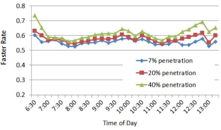
Figure 7: Comparison of FRs at different penetration rates.
Figure 7 shows that over 50% of routes suggested by the balanced routing have shorter travel time than the greedy routing at any interval for any penetration rate in our experiment. Specifically, the average FR for 7%, 20%, and 40% penetration are 55%, 58%, and 61%, respectively. The results demonstrate that the balanced routing provides users with a higher chance to achieve shorter travel time. As the penetration rate increases, FR also rises. Thus, the more users adopt Themis, the higher the prob-ability that users will reduce their trip travel time. Another finding is that even at 7% penetration rate, Themis users could still expect lower travel time, which could be a motivation to change the greedy routing behavior during the bootstrapping stages of Themis.
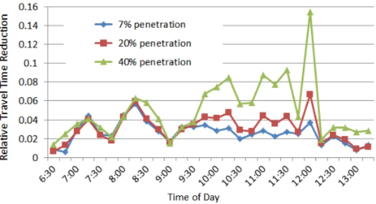
Figure 8 shows that the balanced routing reduces the average trip travel time sub-stantially, e.g., as much as 15% at 40% penetration rate. As expected, the higher the penetration rate is, the lower the trip travel time. Another significant trend of travel time reduction is that RTTR is determined by both the traffic density and the penetra-tion rate. During moderate-traffic hours (10:00 to 12:00), Themis averagely reduces travel time by 8.2% for 40% penetration, 4.0% for 20% penetration, and 2.7% for 7% penetration. These results illustrate that the RTTR achieved by Themis over greedy routing is substantial and increases with the penetration rate for moderate traffic. In addition, the relative travel time reduction increases faster when the penetration rate rises from 20% to 40%. Therefore, better RTTR can be expected when the penetration keeps rising beyond 40%.
During morning commute (6:30 to 9:30) and lunch time (12:30 to 13:00), though the balanced routing still leads to lower average travel time, it is less significant than that in moderate-traffic hours. Moreover, the penetration rate does not have much in-fluence during these intervals. One reason for this result is that these periods represent rush hours in Beijing when most road segments are crowded and there are not many better options to choose even for the balanced routing algorithm. Another reason is that the number of taxis in operation is small at 6:30 and gradually increases to normal level until 9:00, which implies the actual penetration during this period can be lower
Figure 8: Comparison of RTTRs at different penetration rates.
Figure 9: Distribution of RTTRs at 7% penetration.
than daily average value.
After separately analyzing the average values of FR and RTTR in each interval, we combined them by studying the distribution of RTTRs. Figures 9, 10 and 11 illustrate the distribution of RTTRs for all the trips during the experiment period (from 6:30 to 13:00) at different penetration rates.
The common feature of these three histograms is that they are right-skewed, mean-ing that balanced navigation averagely has higher probability to reduce the trip travel time. The most likely result for a driver using balanced navigation is to achieve slightly lower travel time. This is implied by the location of the peak density, which is to the right of the benefit boundary (i.e., RTTR = 0) for each penetration rate. In addition, as the penetration rate rises, the right skew of the histograms tend to be more significant and the peak density tends to move to the right. This means that a higher penetration rate improves both the probability of lowering the travel time and the magnitude of the travel time savings.
Figure 10: Distribution of RTTRs at 20% penetration.
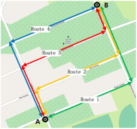
Figure 12: The map of the neighborhood for field experiments.
shorter travel time. However, from the distribution of RTTRs, we found that even if balanced routing sometimes leads to longer travel time, the probability of having a substantial time increase is very small because the density on the left side of the benefit boundary starts from a relatively high value but it drops sharply as RTTR keeps decreasing. In contrast, the density on the right side of the benefit boundary maintains high values until the peek density and then drops at a slower rate than the decreasing rate on the left side of the benefit boundary. This explains why balanced routing has a higher probability to save the drivers’ travel time and implies that the magnitude of the savings are fairly distributed across a large number of vehicles.
6. FIELD EVALUATION
We carried out the field study for cooperative routing by scaling down the exper-imental area to a small neighborhood with sparse background traffic. Compared with the synthetic experiments, the field experiments are capable of evaluating the real in-fluence on traffic rather than the estimated one. The field experiments also have the ability to test the Themis app when users are driving on the roads.
6.1. Experimental Setup and Methodology
During our field study, we recruited 16 volunteers to drive their cars using the Themis app installed on their Android phones. Due to the limited control traffic, one critical issue was how to design the experiment scenarios such that routing with dif-ferent algorithms (i.e., balanced routing vs. greedy routing) would show representa-tive results. We chose a neighborhood shown in Figure 12 to solve this issue: First, the neighborhood provided multiple alternative routes with similar distances, i.e., four possible routes existed between positions A and B. Second, the background traffic was low such that the background traffic conditions were almost identical during the exper-iments for balanced routing and greedy routing. Finally, the majority of road segments
Synchronous Experiments Asynchronous Experiments
Number of Trips 83 86
Mean of the relative errors -0.025 0.003
SD of the relative errors 0.039 0.013
Table 1: The statistic summary of the relative sensing error in the field study
in this neighborhood were one lane and around 50 meters long with stop signs at all intersections. This layout made the average travel delay on the road segments highly depend on the traffic volume even if the number of cars was small. As a result, the experiments conducted in this neighborhood allowed us to observe the performance differences between balanced routing and greedy routing for both traffic distribution and average trip travel time.
We believed that traffic density (i.e., congestion or not) is essentially determined by the vehicles’ arrival rate at a road segment. Therefore, we designed two groups of experiments, synchronous and asynchronous, to mimic high-traffic scenarios and low-traffic scenarios, respectively. During synchronous experiments, all participants submitted routing requests simultaneously to get to B from A. After all the cars had arrived at B, they requested to come back to A simultaneously. The synchronization ensured higher vehicle arrival rate even if the total number of vehicles was small. In the asynchronous experiments, all the setups were the same except that the drivers freely drove from A and B and then came back without synchronization at either positions.
For both groups of experiments, we started with the balanced navigation mode and after 15 minutes switched to greedy routing mode. Out of the 16 experimental cars, 14 submitted routing requests and followed the navigation while the other two traveled around the neighborhood to collect traffic reports from the road segments where no experimental vehicle traveled. The position report frequency was set to 30 seconds. The Traffic Sensing server updated the traffic information every 5 minutes (i.e., traffic estimation interval was 5 minutes).
We defined the trip from A to B as to-trip, and the trip from B to A as return-trip. For both to-trips and return-trips, there were four possible routes (as shown in Figure 12). We named the eight routes using the route id and direction; for example, “route_1_to” referred to the trip from A to B taking route 1.
6.2. Sensing Accuracy
Similar to the synthetic experiments, we first tested the accuracy of the participatory traffic sensing. We compared the ETA of a path shown to the drivers with the actual travel time (ATA) of the same path in the previous interval, as ETA is computed based on the location reports from the previous interval. For each pair of ATA and ETA, we computed the relative error.
The statistics summary for each group of experiments (i.e., synchronous and asyn-chronous) is presented in Table 1. These results confirm the results from the synthetic experiment: a low relative error is observed, which proves the high accuracy of the Themis participatory sensing algorithm. Note that the synchronous experiments show slightly higher error rate. This is due to the fact that the variation of the actual travel
Figure 13: Distribution of total travel time in the synchronous experiment
Figure 14: Distribution of total travel time in the asynchronous experiment
times of different cars is larger in synchronous experiments because of the stronger queueing effect at each intersection or stop sign.
6.3. Traffic Distribution and Trip Travel time
Figure 13 and Figure 14 compare the total travel time of all the cars as well as the travel time distribution on each route under balanced routing and greedy routing for the synchronous and asynchronous experiments, respectively. In each interval, the first bar indicates the results of balanced routing, while the second bar represents the results of greedy routing.
In each figure, since traffic conditions are not recomputed within each interval, greedy navigation assigns traffic to only one to- or return- route with the lowest ETA. On the other hand, balanced navigation reduces the travel time significantly by bal-ancing the traffic load on different alternatives. By checking the ETA of each route in Themis, we also find the balanced navigation to favor the routes with shorter ETA
or the routes sharing less road segments with the other alternatives. Compared with the results from the synthetic experiments, both groups of field experiments got higher time savings under relatively low traffic density. This is partly due to the fact that the neighborhood we choose has the ideal layout for balanced routing, i.e., it has multiple, almost equivalent routes between the origin and the destination. In addition, the high penetration rate also help to bring about better time savings.
The comparison between Figure 13 and Figure 14 shows that the ratio of reduced travel time shrinks from 32% to 13.5%. This can be explained by the fact that the congestion induced by the greedy routing in the asynchronous experiments is alleviated by the lower traffic density (i.e., lower traffic arrival rate than that in the synchronous experiments).
7. LESSONS LEARNED AND FUTURE WORK
Scalability. The Themis system is designed to work in real time. The position samples are processed in every time interval to update the travel speed estimations. The flow-estimation algorithm re-estimates the traffic volume when cars change their travel plans. The cooperative routing module performs the route planning in real time once it receives a new routing request. As a result, the scalability issue is critical.
In the Themis prototype system, since there is one physical server, the request dis-patching of routing and flow monitoring tasks relies primarily on the PHP concurrency. For the traffic sensing task, we launches multiple map-matching and travel time alloca-tion instances to parallelize these two processes. During the synthetic experiment, the server was barely powerful enough to provide real time computation for the experimen-tal area. When the penetration rate is 40%, the average computation time of routing is less than 0.8s. For traffic sensing, as penetration rate does not influence global traffic features (explained in Section 5.1.2), we tested the 7% penetration. The average com-putation time for traffic sensing in an interval is 878s, slightly shorter than the length of the interval, i.e., 900s. While these performance results prove that city-scale balanced routing is not intractable on a single server, the settings in our prototype system will face scalability issues, especially for the traffic sensing tasks, if the covered area or the penetration goes beyond the values we tested (i.e., 65 square kilometers with 7% penetration rate).
Therefore, we plan to explore a parallel implementation for Themis and dispatch the tasks onto multiple machines. The participatory traffic sensing is an ideal “map-reduce” model, where the map-matching and travel time allocation process for each car are the “map” tasks and travel time aggregation for groups of cars are the “reduce” tasks. The flow estimation is done on each road segment, and thus, the map could be partitioned and processed in parallel. In addition, each component is isolated, with data being exchanged only through the shared databases. For instance, the cooperative routing algorithm executes merely on the data from the traffic database and the footprint database. Therefore, the scalability of the balanced routing system mainly relies on the concurrency of the databases, which has been extensively studied (e.g., NoSQL databases).
Balanced Routing Algorithms. The Themis system implemented the EBkSP algo-rithm as a first step, and we used this algoalgo-rithm as an example to compare the
perfor-mance of the balanced routing and the greedy routing. As discussed in Section 2, most cooperative routing algorithms require similar information as EBkSP. Consequently, they can also be implemented into Themis easily and evaluated using the same meth-ods described in Section 5.
By choosing the least popular route, EBkSP increases the entropy of the sub traffic system containing only the planned alternative routes, and consequently, increases the entropy of the whole system, which relates to the system-wide degree of balance. Based on this heuristic, EBkSP is lightweight and performs well. However, during our field study, we found it difficult to translate the meaning of each score into a simple metric understood by drivers. Our test drivers believed this was critical in the successful adoption of the system. In addition, the optimality of EBkSP is not proven even if 100% penetration rate is assumed. We plan to investigate more human acceptable solutions to solve the balanced routing problem. For example, the additional delay incurred to other drivers could be defined as a more meaningful score to minimize the global travel time. Moreover, frequent taxi trajectories could be used as alternatives to incorporate taxi drivers’ intelligence.
Bootstrapping the system.During the initial deployment of Themis, there might not be enough users to sense the city-scale traffic conditions or to collect plenty of routing requests. However, the participatory traffic sensing algorithm in Section 3.2 and the background traffic estimation algorithm in Section 3.3 can also be used in conjunction with external datasets. For example, many taxi companies sell their real-time trajectory data. For the traffic sensing task, the Themis system can also utilize popular online services such as Google Maps [3] or Waze [4] to get their ETAs.
Since Themis reduces the global traffic volume and travel time, it could be useful to prevent congestion and reduce pollution. The governments may want to incentivize drivers to participate by rewarding the users who contribute to a better traffic ecosys-tem. For instance, drivers who usually take high-scored route may receive discounts for their vehicle registration. We believe this approach will help build a friendly traffic ecosystem and ideally lead the traffic system to its system optimum.
8. CONCLUSION
This article presents the design, implementation, and evaluation of Themis, a practi-cal balanced traffic routing system that supports cooperative routing algorithms. To the best of our knowledge, Themis is the first stand-alone navigation system & phone app providing cooperative routing services. Themis collects traffic data from the participat-ing drivers and accurately estimates the real-time traffic conditions and the anticipated traffic volume.
We build a Themis prototype, consisting of an Android app and a backend serv-er, and carry out field studies to validate its feasibility. More importantly, a synthetic evaluation method is presented to investigate the performance of Themis at different penetration rates based on real-life trajectory dataset. The city-scale synthetic experi-ments using data from 26,000 taxis demonstrate that balanced routing can reduce the average travel time in the road network and alleviate congestion. The benefits of bal-anced routing over greedy routing emerge even at low penetration rates. In addition,
the performance variations at different penetration rates consolidate the hypothesis that cooperative routing provides more benefits when the penetration rates are higher.
ACKNOWLEDGMENT
We thank the anonymous reviewers for their valuable and insightful comments. This work was supported in part by the National Science Foundation grants CNS-1111811 and CNS-1409523, and by a Google Research Award.
References
[1] Ericsson ConsumerLab, “From apps to everyday situations - an ericsson con-sumer insight study,” Tech. Rep., 2011.
[2] A. Malm, “Mobile navigation services and devices - 6th edition,” Berg Insight, Tech. Rep., 2013.
[3] “Google Maps,” http://www.google.com/mobile/maps/. [4] “Waze,” http://www.waze.com/.
[5] W. Sha, D. Kwak, B. Nath, and L. Iftode, “Social vehicle navigation: integrating shared driving experience into vehicle navigation,” in Proceedings of the 14th Workshop on Mobile Computing Systems and Applications. ACM, 2013, p. 16. [6] R. K. Ganti, N. Pham, H. Ahmadi, S. Nangia, and T. F. Abdelzaher, “GreenGPS: a participatory sensing fuel-efficient maps application,” inProceedings of the 8th international conference on Mobile systems, applications, and services. ACM, 2010, pp. 151–164.
[7] J. D. Murchland, “Braess’s paradox of traffic flow,” Transportation Research, vol. 4, no. 4, pp. 391–394, 1970.
[8] D. Buscema, M. Ignaccolo, G. Inturri, A. Pluchino, A. Rapisarda, C. Santoro, and S. Tudisco, “The impact of real time information on transport network routing through intelligent agent-based simulation,” inScience and Technology for Hu-manity (TIC-STH), 2009 IEEE Toronto International Conference. IEEE, 2009, pp. 72–77.
[9] T. Roughgarden,Selfish routing and the price of anarchy. MIT press, 2005. [10] T. Yamashita, K. Izumi, and K. Kurumatani, “Car navigation with route
infor-mation sharing for improvement of traffic efficiency,” inIntelligent Transporta-tion Systems, 2004. Proceedings. The 7th InternaTransporta-tional IEEE Conference on, Oct 2004, pp. 465–470.
[11] D. Wilkie, J. P. van den Berg, M. C. Lin, and D. Manocha, “Self-aware traffic route planning.” inAAAI, 2011.
[12] S. Lim and D. Rus, “Stochastic distributed multi-agent planning and applications to traffic,” inRobotics and Automation (ICRA), 2012 IEEE International Confer-ence on. IEEE, 2012, pp. 2873–2879.
[13] R. Kanamori, J. Takahashi, and T. Ito, “Evaluation of anticipatory stigmergy s-trategies for traffic management,” inVNC, 2012, pp. 33–39.
[14] P.-J. He, K.-F. Ssu, and Y.-Y. Lin, “Sharing trajectories of autonomous driving vehicles to achieve time-efficient path navigation,” inVNC, 2013, pp. 119–126. [15] A. van den Bosch, B. van Arem, M. Mahmod, and J. Misener, “Reducing time
delays on congested road networks using social navigation,” inIntegrated and Sustainable Transportation System (FISTS), 2011 IEEE Forum on. IEEE, 2011, pp. 26–31.
[16] J. Pan, M. A. Khan, I. S. Popa, K. Zeitouni, and C. Borcea, “Proactive vehicle re-routing strategies for congestion avoidance,” inDistributed Computing in Sensor Systems (DCOSS), 2012 IEEE 8th International Conference on. IEEE, 2012, pp. 265–272.
[17] P. T. Harker, “Multiple equilibrium behaviors on networks,”Transportation Sci-ence, vol. 22, no. 1, pp. 39–46, 1988.
[18] B. Greenshields, J. Bibbins, W. Channing, and H. Miller, “A study of traffic ca-pacity,” inHighway research board proceedings, vol. 1935. National Research Council (USA), Highway Research Board, 1935.
[19] Board of Public Roads, “Traffic assignment manual for application with a large, high speed computer,” Tech. Rep., 1964.
[20] J. Aslam, S. Lim, and D. Rus, “Congestion-aware traffic routing system using sen-sor data,” inIntelligent Transportation Systems (ITSC), 2012 15th International IEEE Conference on. IEEE, 2012, pp. 1006–1013.
[21] P. Newson and J. Krumm, “Hidden markov map matching through noise and sparseness,” inProceedings of the 17th ACM SIGSPATIAL International Confer-ence on Advances in Geographic Information Systems. ACM, 2009, pp. 336– 343.
[22] J. Aslam, S. Lim, X. Pan, and D. Rus, “City-scale traffic estimation from a rov-ing sensor network,” inProceedings of the 10th ACM Conference on Embedded Network Sensor Systems. ACM, 2012, pp. 141–154.
[23] V. Akgun, E. Erkut, and R. Batta, “On finding dissimilar paths,”European Jour-nal of OperatioJour-nal Research, vol. 121, no. 2, pp. 232 – 246, 2000.
[24] “OsmAnd Maps and Navigation,” http://osmand.net/. [25] “OpenStreetMap,” http://www.openstreetmap.org/. [26] “PostgreSQL,” http://www.postgresql.org/.
[27] “osm2pgrouting,” https://github.com/pgRouting/osm2pgrouting/. [28] “pgRouting,” http://pgrouting.org/.