Cross-domain sentiment classification using grams derived from syntax trees and an adapted naive Bayes approach

(1)

CROSS-DOMAIN SENTIMENT CLASSIFICATION USING GRAMS DERIVED FROM SYNTAX TREES AND AN ADAPTED NAIVE BAYES APPROACH

by

SRILAXMI CHEETI

B.Tech, Jawaharlal Nehru Technology University (JNTU), India, 2008

A THESIS

submitted in partial fulfillment of the requirements for the degree

MASTER OF SCIENCE

Department of Computing and Information Sciences College of Engineering

KANSAS STATE UNIVERSITY

Manhattan, Kansas

2012

Approved by: Major Professor Doina Caragea

(2)

Abstract

There is an increasing amount of user-generated information in online documents, includ-ing user opinions on various topics and products such as movies, DVDs, kitchen appliances, etc. To make use of such opinions, it is useful to identify the polarity of the opinion, in other words, to perform sentiment classification. The goal of sentiment classification is to classify a given text/document as either positive, negative or neutral based on the words present in the document. Supervised learning approaches have been successfully used for sentiment classification in domains that are rich in labeled data. Some of these approaches make use of features such as unigrams, bigrams, sentiment words, adjective words, syntax trees (or variations of trees obtained using pruning strategies), etc. However, for some domains the amount of labeled data can be relatively small and we cannot train an accurate classifier using the supervised learning approach. Therefore, it is useful to study domain adaptation techniques that can transfer knowledge from a source domain that has labeled data to a target domain that has little or no labeled data, but a large amount of unlabeled data. We address this problem in the context of product reviews, specifically reviews of movies, DVDs and kitchen appliances. Our approach uses anAdapted Na¨ıve Bayes classifier(ANB) on top of the Expectation Maximization (EM) algorithm to predict the sentiment of a sentence. We use grams derived from complete syntax trees or from syntax subtrees as features, when training the ANB classifier. More precisely, we extract grams from syntax trees correspond-ing to sentences in either the source or target domains. To be able to transfer knowledge from source to target, we identify generalized features (grams) using the frequently co-occurring entropy (FCE) method, and represent the source instances using these generalized features. The target instances are represented with all grams occurring in the target, or with a reduced grams set obtained by removing infrequent grams. We experiment with different types of

(3)

grams in a supervised framework in order to identify the most predictive types of gram, and further use those grams in the domain adaptation framework. Experimental results on several cross-domains task show that domain adaptation approaches that combine source and target data (small amount of labeled and some unlabeled data) can help learn classifiers for the target that are better than those learned from the labeled target data alone.

(4)

List of Figures

3.1 Syntax tree generated using Stanford parser . . . 16

3.2 MCT for sentiment word “treasure” . . . 18

3.3 PT for sentiment word “treasure” . . . 18

3.4 MCT for sentiment word “brisk” . . . 19

3.5 PT for sentiment word “brisk” . . . 19

3.6 MCT or combined tree using sentiment based pruning strategy . . . 20

3.7 PT or combined tree using sentiment based pruning strategy . . . 21

3.8 E1 and E2 nodes for adjective word “brisk” . . . 23

3.9 E1 and E2 nodes for adjective word “familiar” . . . 24

3.10 MCT for sentiment word “brisk” using adjective based pruning strategy . . . 25

3.11 PT for sentiment word “brisk” using adjective based pruning strategy . . . . 25

3.12 MCT for sentiment word “familiar” using adjective based pruning strategy. . 26

3.13 PT for sentiment word “familiar” using adjective based pruning strategy. . . 26

3.14 Combined MCT using adjective based pruning strategy . . . 27

3.15 Combined PT using adjective based pruning strategy . . . 28

3.16 Syntax tree generated using the Stanford parser . . . 29

3.17 PT subtree generated using sentiment based pruning strategy . . . 29

3.18 PT subtree generated using adjective based pruning strategy . . . 30

3.19 All grams with leaf nodes . . . 30

3.20 Unigrams with leaf nodes . . . 31

3.21 Unigrams without leaf nodes . . . 31

(7)

List of Tables

4.1 Customer review dataset . . . 50

4.2 Number of all grams with leaf nodes as grams inM, D,D0 andK, respectively 51 4.3 Number of unigrams with leaf nodes as grams in M and D0 . . . 52

4.4 Number of unigrams with leaf nodes as grams in M,D and K . . . 52

4.5 Number of unigrams without leaf nodes as grams in M, D,D0,K . . . 52

4.6 Number of all unigrams as grams in M, D,D0,K . . . 52

4.7 Number of all grams with leaf nodes as PT grams in M, D, K . . . 52

4.8 Number of unigrams with leaf nodes as PT grams in M, D, K . . . 52

5.1 Results for Experiment 1: domain specific classifiers using SVM and trees . . 53

5.2 Results for Experiment 2: domain specific classifiers using SVM and grams from FT . . . 54

5.3 Results for Experiment 2: domain specific classifiers using SVM and grams from PT-SPS . . . 55

5.4 Results for Experiment 2: domain specific classifiers using NBM and grams from FT . . . 55

5.5 Results for Experiment 2: domain specific classifiers using NBM and grams from PT-SPS . . . 55

5.6 Results using unigrams with leaf nodes as grams for Source D0 and Target M 58 5.7 Results using unigrams with leaf nodes as grams for Source M and Target D0 59 5.8 Results using unigrams with leaf nodes as grams for Source M and Target D 60 5.9 Results using unigrams with leaf nodes as grams . . . 62

5.10 Results using all grams with leaf nodes as grams . . . 64

5.11 Results using unigrams without leaf nodes as grams . . . 65

5.12 Results using all unigrams as grams . . . 66

5.13 Results using all grams with leaf nodes as grams from PT-SPS . . . 68

(8)

Acknowledgments

While this thesis is my own work, it benefited from the insights and direction of several people. I would like to thank them all for their help and support.

First and foremost, I would like to express my deepest gratitude to my advisor, Dr. Doina Caragea, for her excellent guidance, caring, patience, and for providing me with an excellent atmosphere for doing research. Without her guidance and persistent help this thesis would not have been possible. I would like to thank her for all the valuable discussions and inputs she provided during the last two years. Her patience and support helped me overcome many crisis situations and finish this thesis. Throughout my studies at KSU, she provided encouragement, sound advice, good teaching, good company, and lots of great ideas. I would have been lost without her.

I would like to thank Dr. Amtoft Torben for being a member of my M.S. committee, and for educating me about some of the important concepts in algorithms and about ways to tackle some of the hardest problems.

I would also like to thank Dr. Mitchell L. Neilsen, for being a member of my M.S. committee. His classes are a great source of information and motivate students to think of simple solutions for some of the most challenging problems in real time operating systems. I would like to thank my family members, Mr. Cheeti Hanmantha Rao, Mrs. Cheeti Rama Devi and my brother Mr. Cheeti Srinivas for their love and support at every stage of my life. It is because of their support and encouragement that I am able to complete my Masters. I would also like thank my friends and colleagues especially Sandeep Solanki, Karthik Tangirala, Ana Stanescu, Nic Herndon for helping me in the early days of my M.S. studies and for valuable discussions.

Finally, I would like to thank my husband, Kalyana Koka. He was always there cheering me up and stood by me through the good and bad times.

(9)

Chapter 1

Introduction

In this chapter, we will first provide some motivation for the sentiment analysis problem in Section 1.1. We state the problem addressed and emphasize challenges of this problem in Section 1.2. Finally, we give an outline of the proposed approaches in Section 1.3.

1.1

Motivation for Sentiment Classification

The amount of information available on the web is increasing tremendously every day. Some of this information is provided by internet users in the form of reviews, blogs, webpages, etc., and can be useful for other users or for companies targeting internet users. For example, product reviews contain information that can be helpful in the decision making process of new customers looking for various products. Assuming that several companies such as Sony, Canon, Nikon make the same product (e.g., camera), a customer might be interested in buying the best camera available, within a particular price range, regardless of the producing company. In order to pick the best camera, that customer needs to know what are the pros and cons of the cameras made by different companies. In other words, the customer needs to classify the online information (i.e., the reviews) as positive, negative or neutral.

Similarly, customer reviews can be useful for the companies manufacturing products, as they can learn about customer’s likes and dislikes and adjust the products accordingly, or use that information to train recommender systems to recommend products to users. For example, companies like Amazon, Motorola, ATT, Verizon can identify reviews and classify

(10)

them as positive, negative or neutral. This information will help companies to come up with ideas for new features that the customers are looking for, which, in turn, can result in an increase in the revenue for the company. Furthermore, companies can also use the information that is available online to provide recommendations related to products, movies, restaurants, maps, good community schools, etc. based on the likes and dislikes of a person. Manually classifying customer reviews can be an intensive, time consuming process, as it requires a lot of browsing and reading of reviews. Therefore, automated tools to do this classification are greatly needed, as they could save both customers and companies a lot of time and quickly provide the gist of the reviews about a product. Automated classification of online data as positive, negative or neutral is known as sentiment classification, an area at the intersection of Machine Learning (ML) and Natural Language Processing (NLP). In this context, a sentiment classification problem is formulated as a machine learning problem, where labeled training data is provided to a learning algorithm and a classifier is learned. The resulting classifier can then predict the sentiment of new unlabeled data. Both training and test instances are represented using automatically generated features, including NLP features.

1.2

Problem Addressed and Challenges

Sentiment classification, in general, is a broad problem, which can be addressed at various levels. For example, we can talk about sentiment classification at word level, sentence level or document level. Much of the previous sentiment classification work has been done at the document level using keyword based approaches, and there has not been a lot of work done at sentence level. Sentence level classification is more difficult when compared to document level classification because classification of a sentence as positive, negative or neutral has to be performed in the absence of context. This problem can be alleviated, if two or more consecutive sentences are combined together, or if the whole document is used. Another challenge in sentiment classification is that a sentence (and for that matter a document) can

(11)

have more than one sentiment.

In this work,we focus on sentiment classification at sentence level, but consider sentences that have only one sentiment. We aim to use machine learning approaches to address this problem. Generally, with enough training data this approach is feasible and can result in accurate domain specific classifiers. For example, we can use movie review data to learn a movie sentiment classifier and use it to predict the sentiment of new movie reviews. However, in real world applications, the amount of labeled data for a particular domain can be limited and it is interesting to consider cross-domain classifiers, in other words, classifiers that can be used on a target domain, but are learned from both target and another source domain. For example, we can use books as the source domain, while the target domain can be either music, DVDs, movies, electronics, clothing, toys, etc.

Generally, a classifier built on one domain (i.e., source domain) does not perform well when used to classify the sentiment in another domain (i.e., target domain). One reason for this is that there might be some specific words that express the overall polarity of a given sentence in a given domain, and the same words can have different meaning or polarity in another domain. Let us consider kitchen appliances and cameras as our domains, then words such as good, excellent express positive sentiment in both kitchen appliance domain, as well as camera domain. Words such as bad, worseexpress negative sentiment across both kitchen appliance and camera domains. However, words such as tasteful, tasteless express sentiments in kitchen appliance domain and may or may not express any sentiment in the camera domain. Words such as lens, sleek, megapixel express sentiment in camera domain and may or may not express any sentiment in the kitchen appliance domain. In cross-domain classification problems, the general goal is to leverage labeled data in the source domain and, possibly, some labeled data in the target domain, together with unlabeled data from the target. Under this scenario, we aim to learn cross-domain classifiers (at sentence level) for predicting the sentiment of target instances by using data available in both source and target domains.

(12)

The cross-domain sentiment classification problem presents additional challenges com-pared to the corresponding problem in a single domain. Using both source and target data to construct the classifier requires a lot of insight and effort, specifically with respect to how to choose source features that are predictive for target, and also how to combine data or clas-sifiers from source and target. To address the first problem, most previous approaches [Pan et al., 2010], [Blitzer et al., 2007], [Tan et al., 2009] identify domain independent features (a.k.a., generalized or pivot features) to represent the source, and domain specific features to represent the target. Domain independent features serve as a bridge between source and target, thus reducing the gap between them. The performance of the final classifier will heavily depend on the domain independent features, therefore, care must be used when selecting these features.

In our work, we used NLP syntax structured trees to generate features. Domain inde-pendent features are selected based on the frequently co-occurring entropy (FCE) method proposed by Tan et al. [2009]. Features with high entropy values as assumed to be gener-alized features and used to represent the source domain. Furthermore, to combine source and target data, we use an EM based na¨ıve Bayes classifier proposed also by Tan et al. [2009]. In this approach, as the number of iterations increases, we reduce the weight for the source domain instances while increasing the weight for the target domain instances, so that the classifier can be used for predicting the target domain instances. Originally, the approach in [Tan et al., 2009] assumes labeled source data and unlabeled target data. In our implementation, we can also use labeled target domain data.

1.3

High Level Overview of Proposed Approaches

Our goal is to use features extracted from subtrees of a complete syntax tree or a structured syntax tree to learn machine learning classifiers for predicting the sentiment of customer product reviews in a cross-domain scenario. To learn classifiers, we use an adapted na¨ıve Bayes algorithm (ANB) built on top of the expectation maximization (EM) algorithm.

(13)

In the initial phase of the work, we experimented with complete syntax trees, subtrees of complete syntax trees or path trees as features, in a domain specific scenario, to learn about the predictiveness of such features with respect to the sentiment classification prob-lem. Specifically, we ran several experiments with different kinds of trees as features using supervised machine learning algorithms such as SVM and na¨ıve Bayes. Given the promising results of the syntax trees in a supervised learning framework, we decided to use them also in the domain adaptation framework (i.e., with ANB classifier). As mentioned in the pre-vious section, we used frequently co-occurring entropy method (FCE, as described in [Tan et al., 2009]) to identify generalized features. This method calculates entropy values for features extracted from syntax trees (by comparing their occurrence frequency in target versus source), and ranks them in decreasing order of the entropy values. The top 50 or 100 FCE features are considered to be domain independent features, and are used to represent instances in the source domain.

We used ANB under the following two scenarios:

1. Case 1: Assume that the source domain contains labeled data and the target domain has only unlabeled data.

Here, we first train a classifier using the source domain labeled data and predict the corresponding labels for the target domain unlabeled data. From the second iteration onwards, we train a combined classifier based on the labels predicted in the previous iteration for target domain unlabeled data and source domain labeled data. We use the trained classifier to predict labels for the target domain unlabeled instances. This process is repeated iteratively until we meet a convergence point where we have the same labels for the target domain unlabeled instances for the two consecutive iterations. During this iterative process, we use only the generalized features for the source domain, whereas for the target domain we use the whole vocabulary as features. We perform a 3 fold cross validation on target domain data. More precisely, from the second iteration onwards, we consider 2 folds of the target domain (unlabeled data)

(14)

along with source domain (labeled data) as our training data and use the remaining one fold of the target domain unlabeled data as test data. During the iterative process, we reduce the weight for the source domain instances (thus, decreasing the influence of the source on the final classifier), while increasing the weight for the new target domain instances, in an effort to help predict the target domain instances accurately. 2. Case 2: Assume that the source domain contains labeled data and the

target domain has small amount of labeled data and unlabeled data.

This second case is similar to the first case, except that we used both source domain labeled data along with target domain labeled data instead of using only source domain labeled data as described in Case 1. In Case 2, we perform 3 fold cross validation on target domain as well. Here, from the second iteration onwards, we consider 2 folds of the target domain (labeled and unlabeled data) along with source domain (labeled data) as our training data and use the remaining one fold of the target domain unlabeled data as test data.

The rest of the thesis is organized as follows: Chapter 2 describes the previous work on cross-domain sentiment classification. In Chapter 3, we formulate the problem of sentiment classification and then explain the various approaches that we used in our work, along with some detailed examples. Chapter 4 explains the dataset, experimental setup discussing the various experiments that we have performed and also the research questions that we have addressed. In Chapter 5, we discuss the results of the experiments and explain the usefulness of our proposed approaches for the cross-domain sentiment classification problem. Finally, in Chapter 6 we conclude our work and present directions for future work in Chapter 7.

(15)

Chapter 2

Related Work

This chapter gives detailed information about the previous work on sentiment classification across domains. The information available on the web is growing tremendously day by day. Sentiment classification across domains is very challenging because generally, a classifier trained on one domain cannot predict the instances from a different domain appropriately. This is because domain specific features have different meanings in different domains. The biggest challenge involved in performing sentiment classification experiments depends on selecting features and Machine Learning algorithms to use for different datasets. In this chapter, we will give an overview of various types of features, Machine Learning algorithms, the datasets that were used by various authors with their corresponding results and also the type of classification (either sentence level or document level) that they addressed.

Li and Zong [2008] proposed two approaches for cross-domain sentiment classification. One is the feature level fusion and the other is the classifier level fusion approach. In the feature level fusion approach first, the authors constructed feature sets (f1,f2,f3...) individually in different domains using the training data. Next,Li and Zong[2008] combined all the individual feature sets from different domains into a single feature set (F) and used it to train a classifier. Finally, the authors used this classifier in order to predict the instances from different domains. The disadvantage using this method is that they cannot assign different weights when trying to classify the instances from different domains. For example, if we classify instances from the DVDs domain, then we cannot easily assign higher weights

(16)

to the movie domain and lower weights to the kitchen appliances domain.

In classifier level fusion method, first the authors divided the experimental data into training data (70%), development data (20%) and testing (10%) data. Next, a base clas-sifier is learned individually in different domains using the training data. This approach combines the base classifiers and learns a meta-classifier by applying different methods such as MetaLearning method. During this approach a meta-classifier is trained for each domain, using the development data combined with the output attributes of the base classifiers as input. For example, if we want to learn a meta-classifier for theith _{domain, then we use the}

development data from the ith _{domain along with all the output features from all the base}

classifiers in different domains. Next, to test the data from a particular domain, we use the meta-classifier available from the same domain. MetaLearning will automatically learn the unbalanced information (i.e, assigning higher weights to closely related domains and lower weights to more distinct domains) overcoming the disadvantage from the feature level fusion method. In the experiments performed in this work [Li and Zong, 2008], the datasets cor-respond to four domains: books, DVDs, electronics, and kitchen appliances. The features used are 1gram (unigram), 2gram (gram), 1+2gram (unigrams and grams with high bi-normal separation scores (BNS) [Forman,2003]) and 1gram + 2gram (unigrams+bigrams). BNS is a new metric defined as F−1(tpr)−F−1(f pr), whereF−1 is the inverse cumulative probability distribution of the standard Normal distribution, tpr is the true positive rate and f pr is the false positive rate. The results show that the classifier level fusion performed better than the feature level fusion because it was able to capture the unbalanced informa-tion between different domains.Li and Zong[2008] have also suggested that 1gram + 2gram features are better than other types of features that they have used in their experiments.

Harb et al. [2008] introduced the AMOD (Automatic Mining of Opinion Dictionaries) approach consisting of the following three phases. The first phase, known as Corpora Acqui-sition Learning Phase, solves a major challenge by automatically extracting the data from the web using a predefined set of seed words (positive and negative terms). The second

(17)

phase, also known as Adjective Extraction Phase, extracts a list of adjective words with positive and negative opinions. The third phase, known as Classification Phase is used to classify the given documents using the adjective list of words extracted in the second phase. The authors used unigrams as AMOD features and then used the list of adjective words to classify the given documents. The training dataset was retrieved from ( http://www. google.com/blogsearch) using a list of seed words for the cinema domain and the test set used was the movie review data from the Natural Language Processing (NLP) Group, Cor-nell University ( http://www.cs.cornell.edu/people/pabo/movie-reviewdata/). Harb et al. [2008] have also experimented with data from the car domain. The result shows that AMOD approach was able to classify the given documents by using a list of adjective words in a single domain.

Blitzer et al. [2007] introduced another domain adaptation strategy, which is an ex-tension of an approach previously proposed by the same authors, called structural corre-spondence learning (SCL) [Blitzer et al., 2006]. This algorithm reduces the relative error due to adaptation between domains and also identifies a measure of domain similarity when compared to the original SCL. Here, the authors first choose a set of features that occur frequently in both source and target domains, also known as pivot features. Next, linear predictors are used to find the correlations between the pivot elements and all other fea-tures in the unlabeled data from both source and target domains. The performance of this algorithm depends on the selection of the pivot features. The pivot features should be good predictors of source domain labeled data. It is very important which features to consider as pivot features because they should be helpful to predict the target unlabeled instances based on the classifier learned from both the source and target domains. The pivot features are the target features that have the highest mutual information (MI) to the source domain label. The dataset used is an Amazon product reviews dataset and consists of four differ-ent products: books, DVDs, electronics and kitchen appliances. The authors assume that source domain dataset contains labeled and unlabeled data, whereas target domain dataset

(18)

contains only unlabeled data. They observe that choosing the pivot features using MI has reduced the relative error by 36%. Furthermore, when introducing 50 labeled instances from the target domain, the observed average reduction in error is 46%. Overall, the algorithm is found to be very useful for cross-domain sentiment classification especially due to the use of the MI to select the pivot features.

Pan et al.[2010] proposed Spectral Feature Alignment (SFA) algorithm for cross-domain sentiment classification. The process of selecting the pivot features is same as described by Blitzer et al. [2007]. However, the gap between the domains is reduced by constructing a bipartite graph and by adapting the spectral clustering techniques. The experimental dataset consists of Blitzer, Amazon, Yelp and City-search. Blitzer dataset [Blitzer et al., 2007] contains reviews for four product domains: books, DVDs, electronics and kitchen ap-pliances. The dataset collected from Amazon, Yelp and City-search consists of three product domains: video games, electronics and software. In [Pan et al., 2010], sentiment classifi-cation is performed at the document level. The features used are the words from different domains. Pan et al.[2010], compared SFA with NoTransf (where a classifier is learned using source domain instances as training data), SCL [Blitzer et al.,2006], LSA [Deerwester et al., 1990] and FALSA (a classifier is trained based on the features learned by applying LSA on the co-occurrence matrix of domain-independent and domain-specific features and used as one of the baselines). They found that SFA [Pan et al., 2010] results are better than those of the other algorithms.

Glorot [2011] introduced a Deep Learning approach to extract the high level features from reviews in the unlabeled data when performing sentiment classification across domains. The Deep Learning algorithm aims to find out the intermediate concepts between the source and target domains. The intermediate concepts might include concepts like product quality, product price, customer service, etc. Here, the authors follow a two step process to perform sentiment classification across different domains. In the first step, they extract the high level features using a Stacked De-noising Auto-encoder (SDA) with rectifier units. The

(19)

SDA is learned in a greedy layer-wise fashion using stochastic gradient descent. In the second step, Glorot [2011] proposes to learn a classifier on the transformed labeled data from the source domain. The features used are unigrams and bigrams. The dataset used is an Amazon dataset with 26 domains. Glorot[2011] found that the Deep Learning approach results are better than the SCL [Blitzer et al., 2006] and SFA [Pan et al., 2010] results.

Zhang et al.[2010] proposed to use different kinds of syntax subtrees as features, where the subtrees are obtained from complete syntax trees by using both adjective and sentiment word pruning strategies. The syntax trees are derived using the Stanford parser. These features were used for single domain sentiment classification and were found to be very useful for the classification tasks considered.

Tan et al. [2009] proposed an adapted na¨ıve Bayes (ANB) algorithm to perform cross-domain sentiment classification. The first step is to find generalized features in order to build a bridge between the source and the target domains. In order to retrieve the generalized features they used a frequently co-occurring entropy (FCE) method and picked the features with the highest entropy values as the generalized features. Next, two classifiers are learned, one from the source domain using only the generalized features from the source domain and the other from the target domain using all the features from the target domain. Then, the classifiers are used to predict the target domain unlabeled instances. The process of learning the classifiers and then using them to predict the target domain instances is repeated until a convergence point is met. The study used Chinese domain-specific datasets: Education Reviews (Edu, from http://blog.sohu.com/learning/), Stock Reviews (Sto, from http: //blog.sohu.com/stock/) and Computer Reviews (Comp, fromhttp://detail.zol.com. cn/). The ANB algorithm is compared with Na¨ıve Bayes (supervised baseline), EM-based Na¨ıve Bayes (semi-supervised baseline), Na¨ıve Bayes Transfer Classifier (transfer-learning baseline) and the results show that ANB performs much better than the other algorithms.

As explained earlier, our goal is to perform sentence level sentiment classification across domains. From the above mentioned previous works, we came to know that features used

(20)

with classifiers play a vital role in classification tasks. We can select either unigrams, bigrams, 1+2Gram, 1Gram+2Gram, adjective words, sentiment words or structured syntax trees as features for our classification tasks. In our work, we use different kinds of syntax subtrees as features as discussed in detail in [Zhang et al., 2010].

We have seen that there are many different kinds of algorithms such as feature level fusion, classifier level fusion [Li and Zong, 2008], SCL [Blitzer et al., 2006], AMOD [Harb et al., 2008], SFA [Pan et al., 2010], Deep Learning [Glorot, 2011], ANB [Tan et al., 2009] that can be applied to the cross-domain classification problem. Previous work (such as Pan et al. [2010], Blitzer et al. [2006]) suggested that the generalized features can be selected by using MI, FCE methods, among others. We have used FCE and ANB as discussed in [Tan et al., 2009] to perform cross-domain sentiment classification in our work. We have extended ANB by including some labeled data from the target domain. Another contribution of this work is the use of different kinds of syntax subtrees as features. The dataset that we use is manually extracted from BestBuy ( https://bbyopen.com/) and Amazon ( http://www.amazon.com/). The manually extracted dataset contains reviews for customer products such as DVDs, movies and kitchen appliances. In our work, we have overcome the disadvantage of having a predefined set of domain specific and domain independent words by using a FCE [Tan et al., 2009] method.

(21)

Chapter 3

Problem Definition and Approaches

This chapter describes the task of sentence level sentiment classification across domains. The chapter is organized as follows: In Section 3.1, we begin by describing some of the terms that we use in our classification problem. In Section 3.2, we give a problem definition with the help of some examples. In Section 3.3, we describe the feature representations and explain how we use them to train classifiers for the problem stated. In Section 3.6, we describe the transfer learning approaches we use for our problem. We also give a detailed description of the approaches, such as pruning strategies, Support Vector Machine (SVM) and Adapted Na¨ıve Bayes (ANB) algorithms, that we have use in this work.

3.1

Basic Terminology

Before we describe the problem addressed, we define the basic terminology used in this work: Domain: A domain is a class consisting of different entities. For example, products such as books, DVDs, electronics, movies, cameras are considered to be different domains. Sentiment Classification: Customers write reviews for various products describing pros and cons, also known as sentiments. These reviews can be in the form of a sentence, a paragraph or a document. From a classifier point of view, the reviews are represented in the form of a bag of words, such as w1, w2, w3,· · · , wn, wherewi ∈ Vocabulary(V). In order to

recommend products to a new customer, we need to know whether the reviews written by the old customers are recommending the product or not. We classify these reviews either

(22)

as positive or negative based on words that were used in these reviews. Thus, in this work we deal with a binary classification problem where a given review can belong to either a positive or a negative class. For any given domain, we denote the total set of sentences in the given domain by S, where s1, s2, s3,· · · , sm ∈ S. For any given sentence sk, where

k ∈ {1,2,3,· · · , m},sk can belong to either a positive or negative class denoted byyk based

on the words present in it. In our work,yk= 1 if the polarity of a given sentence is positive

and yk =−1 if the polarity of a given sentence is negative.

Domain Adaptation: Domain adaptation, a.k.a. cross-domain learning or transfer learn-ing, is used in many areas such as text classification, spam filtering and bioinformatics. The aim of domain adaptation is to learn a model using labeled data from a source domain combined with target domain unlabeled data and, in some cases, a small amount of target labeled data, and to predict the labels for the unlabeled instances from the target domain. In simple terms, we use the information from the source domain together with some informa-tion from the target domain to predict the unlabeled instances in the target domain. Thus, domain adaptation can leverage the knowledge learned from a source domain to the target domain. If the source and the target domains are very close, then the transfer learning is easier; otherwise transfer learning is harder and it may or may not be successful.

3.2

Problem Definition

We denote by Ds the instance distribution over the source domain, and by Dt the instance

distribution over the target domain. We assume that there are M labeled instances in Ds

and N instances in Dt. We explore two scenarios, one where the target domain contains

only unlabeled instances and the other when the target domain contains both labeled and unlabeled instances. Our goal is to learn a classifier that has minimum error with respect to the target domain. In simple words, we try to classify the unlabeled target domain instances as either positive or negative using the combined model learned from both the source domain and the target domain instances. Our instances are review sentences. We

(23)

consider several possible combinations of source and target domains including movie, DVDs and kitchen appliances domains.

3.3

Structured Syntax Trees

As mentioned earlier, we focus on sentence level sentiment classification and build clas-sifiers based on structured syntax trees. For a given sentence, we retrieve its complete syntax tree using the Stanford parser described in [Klein and Manning, 2003]. A syntax tree is an ordered tree consisting of a root node, branch nodes and leaf nodes. Branch or interior nodes are labeled using non-terminals such as S, NP, JJ, as described at http: //en.wikipedia.org/wiki/Parse_tree, whereas leaf nodes are labeled using terminals such as alphabets, numbers, whitespace, special characters. After retrieving the syntax tree, we apply several pruning strategies to extract subtrees from the complete syntax tree, known as structured features. For pruning, we have used a list of sentiment words avail-able at _{http://www.cs.uic.edu/~liub/FBS/sentiment-analysis.html} and a list of ad-jectives available at http://www.enchantedlearning.com/wordlist/adjectives.shtml

to extract the subtrees called Minimal Complete Tees (MCT) and Path Trees (PT). These syntax subtrees are used to represent instances and provided to a supervised SVM classifier. The SVM-Light-TK tool described in [Joachims, 2002] is used for this purpose, as it can handle tree kernels (and thus avoids the need to generate linear tree features explicitly).

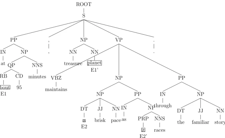
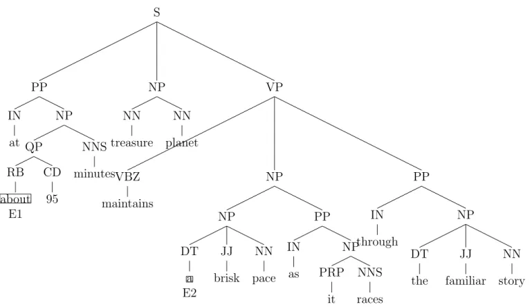
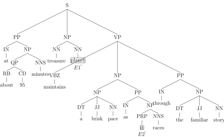
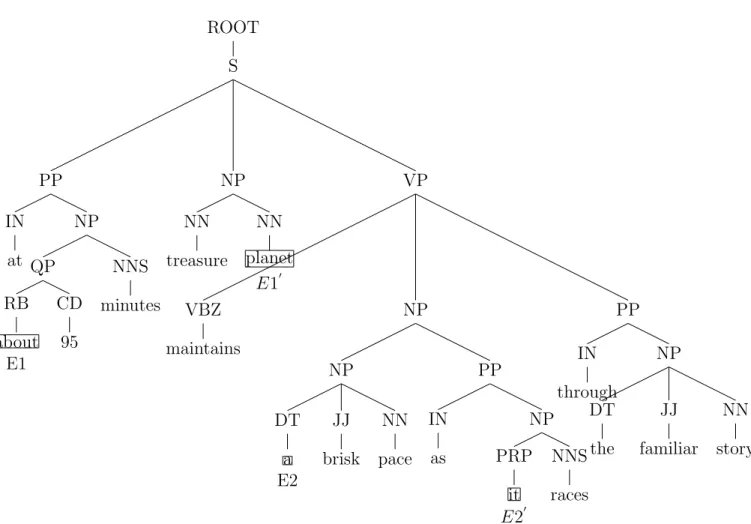
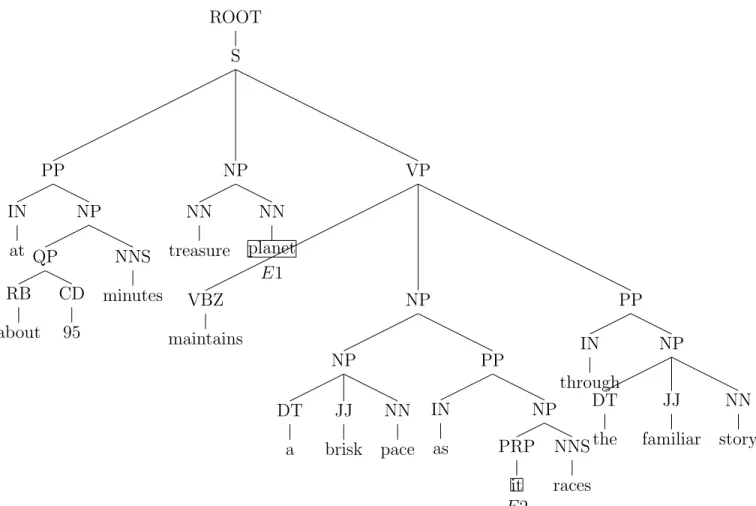
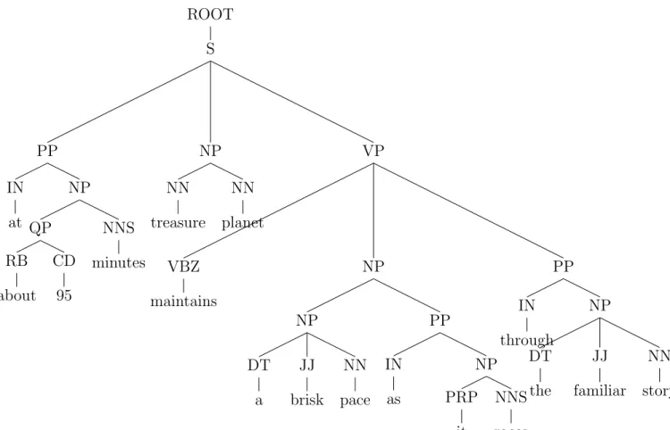
Given the following sentence: ”at about 95 minutes, treasure planet maintains a brisk pace as it races through the familiar story.” - the syntax tree obtained using the Stanford parser is shown in Figure 3.1.

3.3.1

MCT and PT Using Sentiment based Pruning Strategies

First, we will remove the occurrences of (, , ) or (. .) from the syntax tree generated using the Stanford parser. Next, we check whether a sentence has any sentiment words from the list used by Narayanan et al. [2009] available at _{http://www.cs.uic.edu/~liub/FBS/}

(24)

ROOT S PP IN at NP QP RB about E1 CD 95 NNS minutes , , NP NN treasure NN planet E1’ VP VBZ maintains NP NP DT a E2 JJ brisk NN pace PP IN as NP PRP it E2’ NNS races PP IN through NP DT the JJ familiar NN story . .

(25)

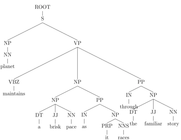
sentiment-analysis.html. The sentiment words for the above sentence are “treasure” and “brisk”. For each sentiment word, we will define two nodes E1 and E2, using a window size of 3, where E1 is marked to the left side and E2 is marked to the right side with respect to the given sentiment word “treasure”. For the sentiment word “treasure”, the E1 node is “about” and the E2 node is “a”, as shown in Figure 3.1, and for the sentiment word “brisk”, the E1 node is “planet” and the E2 node is “it” (shown in Figure 3.1 as E10 and E20). Then, we look at a common parent of E1 and E2 and retrieve the subtree from that common parent, also known as Minimum Complete Tree (MCT) for a given sentiment word. This process is repeated for all the sentiment words in a given sentence. Then, we need to combine the MCT of all the sentiment words by checking for a common node between all the MCT in a given sentence and this resulting subtree is the final version of MCT that we will be using in our work - this tree is also called a combined MCT and reduced some noise present in the complete syntax tree.

But to eliminate further noise from MCT, we apply another pruning strategy to each MCT. During this stage, we prune all the leaf nodes along with their parent nodes that are present to the left side of the node E1, until we hit a common parent between the leaf node and the node E1. Then, we prune all the extra leaf nodes along with their parent nodes that are present to the right side of the node E2, until we hit a common parent between the leaf node and the node E2. The resulting subtree is known as a Path Tree (PT). This process of pruning is repeated for all the MCT trees present in a sentence and the final version of the PT tree is retrieved by finding a common node between all the PT trees available in a given sentence. The MCT for the sentiment word “treasure” is shown in Figure3.2 and the PT for the sentiment word “treasure” is shown in Figure 3.3. The MCT for the sentiment word “brisk” is shown in Figure 3.4 and the PT for the sentiment word “brisk” is shown in Figure 3.5. The combined MCT that we will use in our work for the above sentence is shown in Figure 3.6 and the combined PT is shown in Figure 3.7:

(26)

S PP IN at NP QP RB about E1 CD 95 NNS minutes NP NN treasure NN planet VP VBZ maintains NP NP DT a E2 JJ brisk NN pace PP IN as NP PRP it NNS races PP IN through NP DT the JJ familiar NN story

Figure 3.2: MCT for sentiment word “treasure”

S PP NP QP RB about CD 95 NNS minutes NP NN treasure NN planet VP VBZ maintains NP NP DT a Figure 3.3: PT for sentiment word “treasure”

(27)

S PP IN at NP QP RB about CD 95 NNS minutes NP NN treasure NN planet E10 VP VBZ maintains NP NP DT a JJ brisk NN pace PP IN as NP PRP it E20 NNS races PP IN through NP DT the JJ familiar NN story

Figure 3.4: MCT for sentiment word “brisk”

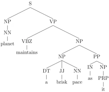
S NP NN planet VP VBZ maintains NP NP DT a JJ brisk NN pace PP IN as NP PRP it Figure 3.5: PT for sentiment word “brisk”

(28)

ROOT S PP IN at NP QP RB about E1 CD 95 NNS minutes NP NN treasure NN planet E10 VP VBZ maintains NP NP DT a E2 JJ brisk NN pace PP IN as NP PRP it E20 NNS races PP IN through NP DT the JJ familiar NN story

(29)

ROOT S PP NP QP RB about E1 CD 95 NNS minutes NP NN treasure NN planet E10 VP VBZ maintains NP NP DT a E2 JJ brisk NN pace PP IN as NP PRP it E20 Figure 3.7: PT or combined tree using sentiment based pruning strategy

(30)

3.3.2

MCT and PT Using Adjective based Pruning Strategy

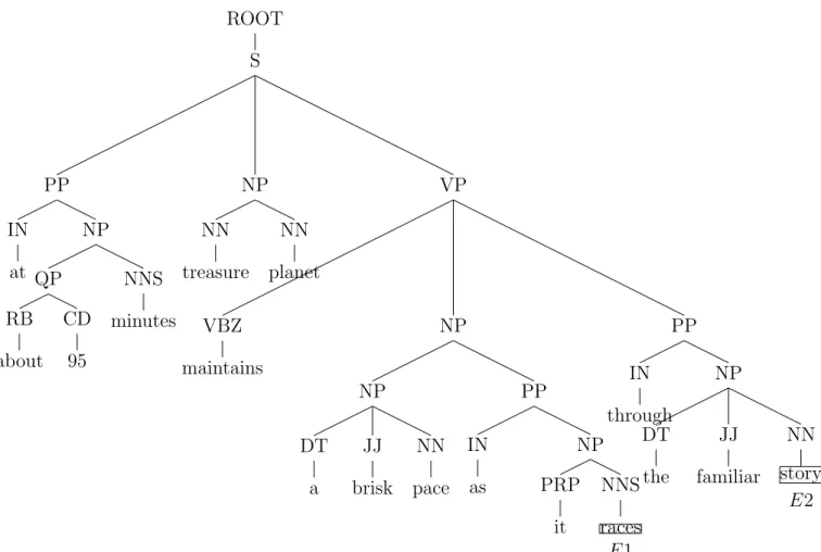
The adjective based pruning strategy is similar to the sentiment word based pruning strategy described in Section 3.3.1, except that in this approach we look for adjective words instead of sentiment words. First, we will check whether a sentence has any adjective words from the list at http://www.enchantedlearning.com/wordlist/adjectives.shtml. Let’s assume the adjective words for the above sentence are “brisk” and “familiar”, then the complete syntax tree is shown in Figure 3.8. For the adjective word “brisk”, the E1 node is “planet” and the E2 node is “it” as shown in Figure3.8. Next, for the adjective word “familiar”, the E1 node is “races” and the E2 node is “story”, as shown in Figure 3.9. Next, the process of extracting MCT, PT, combined MCT and combined PT is exactly same as described in Section3.3.1. MCT for adjective word “brisk” is shown in Figure 3.10and PT for adjective word “brisk” is shown in Figure 3.11. MCT for adjective word “familiar” is shown in Figure 3.12 and PT for adjective word “familiar” is shown in Figure 3.13. The combined MCT for the above sentence using adjective based pruning strategy is shown in Figure 3.14

and combined PT is shown in Figure 3.15:

3.4

Gram Features based on Syntax Trees

Generally, Machine Learning (ML) [Mitchell, 1997] algorithms use feature based repre-sentations for instances, where each instance is represented using a collection of features

f1, f2,· · · , fn. In addition to using structured syntax trees with tree kernels in SVM, we

also use gram features extracted from syntax trees, described in what follows.

Grams are subtrees based on either the complete syntax trees or structured trees gener-ated using pruning strategies. If the original sentence is: “too simple for its own good”- the syntax tree for this sentence is represented in Figure 3.16. The sentiment word present in our given sentence is “good”. The structured PT syntax tree using sentiment word based pruning strategy is shown in Figure3.17. The adjective words are identified as “simple” and “good”. The structured PT syntax tree using adjective based pruning strategy is shown in

(31)

ROOT S PP IN at NP QP RB about CD 95 NNS minutes NP NN treasure NN planet E1 VP VBZ maintains NP NP DT a JJ brisk NN pace PP IN as NP PRP it E2 NNS races PP IN through NP DT the JJ familiar NN story

(32)

ROOT S PP IN at NP QP RB about CD 95 NNS minutes NP NN treasure NN planet VP VBZ maintains NP NP DT a JJ brisk NN pace PP IN as NP PRP it NNS races E1 PP IN through NP DT the JJ familiar NN story E2

(33)

S PP IN at NP QP RB about CD 95 NNS minutes NP NN treasure NN planet E10 VP VBZ maintains NP NP DT a JJ brisk NN pace PP IN as NP PRP it E20 NNS races PP IN through NP DT the JJ familiar NN story

Figure 3.10: MCT for sentiment word “brisk” using adjective based pruning strategy

S NP NN planet VP VBZ maintains NP NP DT a JJ brisk NN pace PP IN as NP PRP it

(34)

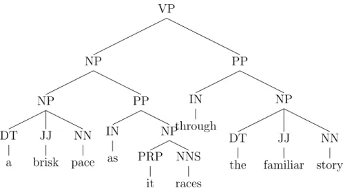
VP NP NP DT a JJ brisk NN pace PP IN as NP PRP it NNS races PP IN through NP DT the JJ familiar NN story

Figure 3.12: MCT for sentiment word “familiar” using adjective based pruning strategy.

VP NP PP NP NNS races PP IN through NP DT the JJ familiar NN story

(35)

ROOT S PP IN at NP QP RB about CD 95 NNS minutes NP NN treasure NN planet VP VBZ maintains NP NP DT a JJ brisk NN pace PP IN as NP PRP it NNS races PP IN through NP DT the JJ familiar NN story

(36)

ROOT S NP NN planet VP VBZ maintains NP NP DT a JJ brisk NN pace PP IN as NP PRP it NNS races PP IN through NP DT the JJ familiar NN story

(37)

ROOT NP ADJP RB too JJ simple PP IN for NP PRP$ its JJ own NN good

Figure 3.16: Syntax tree generated using the Stanford parser PP IN for NP PRP$ its JJ own NN good

Figure 3.17: PT subtree generated using sentiment based pruning strategy

Figure 3.18.

3.4.1

Grams based on Complete Syntax Trees

The following are various types of subtrees (grams) obtained from the complete syntax tree and used as features in our problem.

• All grams with leaf nodes: This type of feature representation has all the possible parent-child subtrees as features, as shown in Figure 3.19.

• Unigrams with leaf nodes: This type of feature representation contains unigram subtrees as features, as shown in Figure 3.20. Unigram consists of one item for any given sequence of words/input. An n-gram consists of n items for any given input. Let’s assume that we have the following input: “too simple for its own good.” The unigrams at word level for the above sentence are: too, simple, for, its, own, good.

(38)

ROOT NP ADJP RB too JJ simple PP IN for NP PRP$ its JJ own NN good

Figure 3.18: PT subtree generated using adjective based pruning strategy

(a) RB too (b) JJ simple (c) IN for (d) PRP$ its (e) JJ own (f) ADJP RB too JJ simple (g) NP ADJP RB too JJ simple (h) NN good (i) NP PRP$ its JJ own NN good (j) PP IN for NP PRP$ its JJ own NN good (k) ROOT NP ADJP RB too JJ simple PP IN for NP PRP$ its JJ own NN good Figure 3.19: All grams with leaf nodes

(39)

(a) RB too (b) JJ simple (c) IN for (d) PRP$ its (e) JJ own (f) NN good Figure 3.20: Unigrams with leaf nodes

(a) ROOT NP (b) NP ADJP (c) ADJP RB (d) ADJP JJ (e) PP IN (f) PP NP (g) NP PRP$ (h) NP JJ (i) ROOT PP (j) NP NN Figure 3.21: Unigrams without leaf nodes

The bigrams at word level for the above sentence are: too simple, simple for, for its, its own, own good. The n-gram at the word level is: too simple for its own good. Here, unigram subtrees are just a pair composed of a parent and their child node, where the child node is a leaf node.

• Unigrams without leaf nodes: This type of feature representation contains all possible unigram subtrees as features except the unigrams with leaf nodes, as shown in Figure3.21. Here, unigram subtrees are just a pair composed of a parent and their child node, where the child node is not a leaf node.

• All unigrams: All possible unigrams present in the syntax tree are taken as features, as shown in Figure 3.22. The combination of unigrams with leaf nodes and unigrams without leaf nodes gives all possible unigrams.

3.4.2

Grams based on Pruned Syntax Subtrees

As we have seen earlier, the PT tree based on sentiment word based pruning strategy is shown in Figure 3.17. Next, we retrieve the different types of grams exactly the same way as described in Section3.4.1except that we have to use PT tree instead of complete (or full) tree. The PT trees based on adjective word based pruning strategy is shown in Figure 3.18.

(40)

(a) ROOT NP (b) NP ADJP (c) ADJP RB (d) ADJP JJ (e) PP IN (f) PP NP (g) NP PRP$ (h) NP JJ (i) ROOT PP (j) NP NN (k) RB too (l) JJ simple (m) IN for (n) PRP$ its (o) JJ own (p) NN good Figure 3.22: All unigrams

We retrieve the different types of grams exactly the same way as described in Section 3.4.1

except that we use the PT tree instead of the complete tree. We can use the complete syntax trees but we are identifying MCT and PT trees because we would like to reduce the noise, a task that is not important for sentiment classification problems.

3.5

Feature Construction for Domain Adaptation

We can select any of these types of grams as features based on their predictive power evaluated using a supervised algorithm in a single domain. Now, the main challenge for performing domain adaptation is to select the features to build a bridge between the source domain and target domain. These features are known as domain independent features. Let us look at the following definitions before discussing about the approach that we used to select the features for building a bridge between the two domains. In our problem we have two domains, source domain and target domain. Each domain has two different kinds of features: domain specific feature and non-domain specific or domain independent feature. These two types of features may be either sentiment or non-sentiment words.

(41)

3.5.1

Domain Specific Features

Domain specific features are those features with specific meaning in either source or target domain. For example: words like thrilling, powerfully acted express sentiment in the movie domain and words such as exceptional control, sleek and distinctive, space-efficient express sentiment in the kitchen appliances domain.

3.5.2

Domain Independent Features

Domain independent features are those features, which have the same meaning in both source as well as target domain. For example: words like good, excellent, bad, worse, etc. are domain independent features.

Why are we interested in domain independent features?

As mentioned earlier domain independent features have the same meaning in both domains source and target domains. The domain independent features are important because these features occur frequently in both domains and can be used in order to transfer knowledge from source to target. Specifically, we learn a classifier based on source domain labeled data along with target domain unlabeled data or on source domain labeled data along with target domain labeled and unlabeled data and use the classifier to predict the labels for target domain unlabeled instances. Source data should be represented using domain independent features, while target data is represented using all features in the target domain (including the specific features), as we want to learn to predict target well.

How do we extract domain independent features?

We used a Frequently Co-occurring Entropy(FCE)method as described byTan et al.[2009] to retrieve the domain independent features, also known as generalized features. This mea-sure satisfies the following two criteria:

a) Independent features occur frequently in both source and target domains; b) Independent features must have similar occurring probability.

(42)

fv = log

Ps(v)∗Pt(v)

Ps(v)−Pt(v)

where fv represents the entropy value for the feature v, Ps(v) is the probability of feature

v occurring in the source domain and Pt(v) is the probability of feature v occurring in the

target domain. Specifically, we have: Ps(v) = (Ns v +α) (Ds+ 2∗α) , Ps(v) = (Nt v+α) (Dt+ 2∗α) where Ns

v and Nvt denote the number of times feature v has occurred in the source domain

and target domain, respectively. Ds and Dt denotes the total number of instances in the

source domain and target domain, respectively. We have used a constant α to avoid any overflow. In our work, α value is set as 0.0001. To avoid the divide by zero error when both the source domain and the target domain probabilities are same, a constant factor β is introduced. After introducing a constant β, the above formula is modified as follows:

fv = log

Ps(v)∗Pt(v)

(Ps(v)−Pt(v)) +β

In our work, β value is set to 0.0001.

3.6

Approaches Used

The following are the various types of machine learning algorithms that are most widely used for classification tasks:

3.6.1

Supervised Learning Algorithms

Supervised algorithms require labeled data, and are very useful when we have a sufficient amount of labeled data to learn a good classifier. In a supervised framework, for a binary problem, we provide a set of training examples, where each example can belong to either a positive class or a negative class. The set of training examples are used to train a model. This

(43)

model will be used to predict new test instances as positives or negatives. The performance is evaluated by comparing the predicted values to the actual values on a hold out dataset. Examples of supervised learning algorithms include: Support Vector Machine (SVM), Na¨ıve Bayes Multinomial (NBM).

Support Vector Machines (SVM)

SVM algorithm is a supervised machine learning algorithm that works very well, especially for binary classification problems. SVM represents each input example as a point in a high dimensional space. If the data is (almost) linearly separable, SVM uses these example points to constructs a hyperplane that separates the positive points from negative points. We can construct many hyperplanes for a given set of example points. The best hyperplane is the one which has the largest separation gap between the positive examples and the negative examples, and this is the hyperplane that SVM finds. New examples are classified to either one of the classes based on which side of the separating hyperplane they fall in, as described in [Cortes and Vapnik, 1995]. When data is not linearly separable in the original space, kernels are used to map the data to a higher dimensional space where data becomes linearly separable. In our work, we used SVM with a tree kernel and a linear kernel in the supervised scenario.

The kernel-based algorithms automatically select the substructures that better describe the subtrees. If the given set of instances are represented in a high dimensional space Z, then the kernel function K is defined as R :Z ×Z →[0,∞], a function which maps a pair of instances x, y ∈X to their similarity score K(p, q). In the following few lines we discuss linear and tree kernels:

1. A linear kernel is the default kernel used by SVM and is very useful when we have many attributes. It is defined as the inner product of the two variables as described in [Cortes and Vapnik, 1995]: R(x, y) = hx, yi=P

ixi·yi

2. A tree kernel [Souza, 2010] is used in order to find the similarity between two syn-tax trees by calculating the dot product of feature vectors in high (or even infinite)

(44)

dimensional feature spaces.

In our work, we use SVM and compare the performance of tree kernels with linear kernels for sentence level sentiment classification in a single domain. Our initial aim is to capture structured information in terms of sub-structures, which acts as an alternative to flat features. To extract the syntactic structured features embedded in a complete parse tree, we use pruning strategies like sentiment word based and adjective word based strategies as described in Section 3.3. In our work we use a tool called SVM-light-tk [Moschitti,2002] which implements tree kernels.

SVM-light-tk has the tree kernel implementation inside SVM-light developed byJoachims [2002]. SV Mlight _{is an implementation of Support Vector Machines in C language. It is}

used for solving binary classification problems. SV Mlight _{consists of two modules: a}

learn-ing module (SVM-learn) and a classification module (SVM-classify). SVM-learn builds a model from the training data. SVM-classify reads this model file and makes predictions on test data instances.

Na¨ıve Bayes Multinomial (NBM)

Na¨ıve Bayes Multinomial is a supervised learning algorithm and it is widely used for doc-ument level classification tasks. It builds the model by using a set of labeled training examples and uses this model to classify the new unlabeled instances. Na¨ıve Bayes Classi-fier is a probabilistic classiClassi-fier and it is based on a strong independence assumption (words in a document are independent given the class label of the document). Furthermore, posi-tions in a sentence are also independent. The NBM algorithm is found to be very useful for text classification, when simply words are used as features. For example, a movie can be classified as a comedy movie if it contains words such as funny, joyful, or humor character names such as Ben Stiller etc. Even though words in a sentence are not dependent, na¨ıve Bayes classifier considers all these words as independent features. In our experiments, we assume that the probability of a gram occurring in a document is totally independent of the gram’s position and its context in a sentence, given the class label of a sentence. In what

(45)

follows, we provide more details of the algorithm.

Let us assume that we are given a document Dto classify as either positive or negative class ck, where ck ∈ {+1,−1}. Using the independence assumption, a document can be

seen as a bag of words (w1, w2,· · · , wn) ∈ D and the word in a document is independent

of its corresponding position and context in a document. Na¨ıve Bayes classifier is based on the Bayes theorem and learning the classifier can be reduced to estimating class prior and the data likelihood. Then, the probability of a class given a document P (ck|D) (posterior

probability) is proportional to multiplying the priorP(ck) and the probabilities n

Y

v=1

P(wv|D).

Finally, we check the probability distributions ofP(ck|D) for all values of k and then classify

the given document in the class which has the highest probability distribution value. The probability of a word given class can be estimated using the following formula as described in [Tan et al., 2009]: P (wv|ck) = Nv∗P (ck|D) + 1 |V| X v=1 Nv∗P (ck|D) +|V|

where wv is a word from a given vocabulary (V) considered as features, ck is the class label

where ck ∈ {+1,−1}, Nv is the number of times word has occurred in a given document D

and |V| is the size of the vocabulary (that contains all the words (w1, w2,· · · , wn)).

We can easily calculate the prior probability in a given document by counting the num-ber of documents with different class labels. The prior probability is calculated using the following formula:

P(ck) =

Number of examples in ck

Total number of examples

Next,P (ck|D) is approximated by multiplying both the prior and the posterior probabilities as follows: P (ck|D)≈P(ck)∗ n Y v=1 P (wv|ck)Nv

(46)

In general, NBM works for a collection of documents. In our work, we used sentences instead of whole documents.

3.6.2

Domain Adaptation Algorithms

Our goal is to reduce the gap between the source and target domains by learning a classifier from source domain and target domain instances to predict the labels for the new target domain unlabeled instances. We use domain adaptation algorithms when we have labeled data in the source domain and little or no labeled data along with unlabeled data in the target domain. We consider two domain adaptation scenarios, as described in what follows: 1. Case 1: Data available is source domain labeled data and only unlabeled data from target domain. In this case, we build a classifier using the source domain labeled data represented with generalized features only. We use the source domain classifier in order to predict the corresponding labels for the target domain unlabeled instances. Next, we build the target domain classifier by using the predicted labels for target domain represented with the whole vocabulary from the target domain as its features. Finally, we use both the source domain classifier and target domain classifier to predict new labels for the unlabeled instances from the target domain and we repeat this process until we meet a convergence point.

2. Case 2: Data available is source domain labeled data, and a small amount of labeled data along with unlabeled data from target domain. In this case, first we build a com-bined classifier using the source domain labeled data and target domain labeled data. Next, we use this classifier in order to predict labels for the unlabeled target domain instances. After predicting the labels for the target domain unlabeled instances, we build another combined classifier using the source domain labeled data, target domain labeled data and the predicted labels for the unlabeled target domain data to predict the labels for the target domain unlabeled instances. This process is repeated until we meet a convergence point.

(47)

The Adapted Na¨ıve Bayes algorithm used to address these two cases is discussed below. The original algorithm works for the first case, but we also adapted it for the second case. Adapted Na¨ıve Bayes (ANB)

ANB [Tan et al., 2009] is a domain adaptation algorithm, based on a weighted transfer version of the na¨ıve Bayes classifier. It builds a classifier using Expectation Maximization (EM) on top of na¨ıve Bayes classifier, to predict the target domain unlabeled instances. One important part of the ANB algorithm is that it simultaneously allows us to reduce the weight given to the source domain instances, while increasing the weight given to the target domain instances at each iteration, by using a constant lambda (λ). This, in turn, allows us to predict the labels for the target domain instances.The EM algorithm is used to find the maximum likelihood. It consists of two steps: E-step (Expectation-step) and M-step (Maximization-step). In the E-step, we estimate the missing data (in our case, the labels of the unlabeled target data) and the model parameters given the observed or known data. In the M-step, we try to maximize the likelihood function by assuming that the missing data is known. The two steps are repeated until we reach a convergence point.

The EM approach used in ANB and described in [Tan et al., 2009] is different from the traditional EM approach because we want to find the maximum likelihood only for the target domain instances but not for the source domain. ANB algorithm achieves this by increasing the weight for the target-domain data, while decreasing the weight for the source-domain data at each iteration. Also, remember that we do not use all the features available in the source domain. We use only a small amount of features also known as generalized features from the source domain because our goal is to classify the target domain instances, but not the source domain. So, in each iteration we use only generalized features for the source domain, whereas we use the whole vocabulary for the target domain. This helps us to improve the prediction ability of the classifier to classify the target domain instances because the domain specific features from the source domain are not very useful for predicting the target domain instances.

(48)

In the following lines, we give the detailed formulas under domain adaptation setting using the ANB classifier on top of EM as described by Tan et al. [2009]:

E-step: P(ck|si)∝ P(ck) Y v∈V (P (fv|ck))Nv,i M-step: P(ck) = (1−λ)∗X i∈Ds P (ck|si) +λ∗ X i∈Dt P (ck|si) (1−λ)∗ |Ds|+λ∗ |Dt| P (fv|ck) = (1−λ)∗ ηs v ∗Nv,ks +λ∗ Nt v,k + 1 (1−λ)∗ |V| X v=1 ηs_v∗N_v,ks +λ∗ |V| X v=1 N_v,kt +|V|

1. Case 1: During the first iteration Dt ∈Dt lab in the above M-step. From the second

iteration onwards Dt ∈Dt lab, Dt unlab until we reach a convergence point.

2. Case 2: During the first iteration Dt = φ in the above M-step. From the second

iteration onwards Dt ∈Dt unlab until we reach a convergence point.

where Ns

v,k and Nv,kt denote the number of appearances of feature fv in source domain and

target domain for its corresponding class ck. These are obtained as follows:

Ns v,k = X i∈Ds N_v,is ∗P (ck|si) , Nt v,k = X i∈Dt N_v,it ∗P (ck|si)

where λ is a parameter for controlling the weights for the source domain versus target domain. The value of λ changes with the number of iterations (τ), which is expressed as: λ = min (δ∗τ,1) and τ ∈ {1,2,3,...} until we reach the convergence point. Here, δ is a constant and in our work we used δ = 0.2. ηs

v is a constant and is given as:

η_vs =

0 if fv ∈/ VF CE

1 if fv ∈VF CE

The time complexity for ANB algorithm is O(nm), where n is the number of examples and m is the number of attributes. However, the complexity of the EM step is O(nmk), where k is the number of iterations.

(49)

Chapter 4

Experimental Setup

In this chapter, we explain the research questions that we have addressed in our work, the dataset used and the experiments designed to evaluate our approach. We have conducted experiments with various classifiers and with variable amount of data to investigate the performance of the classifiers for domain classification within a single domain and across domains. Specifically, this chapter is organized as follows: In Section4.1, we describe various research questions that we have addressed. In Section4.2we list the set of experiments that have performed performed. In Section 4.3, we describe the dataset used.

4.1

Research Questions

The following are the research questions that we have addressed in this work:

• Are the grams extracted from syntax trees, when used as features in a domain specific classifier, comparable in terms of prediction and accuracy to the structured syntax subtrees? Overall, how useful are these features for the sentence-level sentiment clas-sification problem?

According to Zhang et al. [2010], structured features give very good results in terms of accuracy for sentence-level sentiment classification. However, for our domain adap-tation algorithm, ANB, we need to provide features in terms of gram counts. That is possible, when considering the gram based features described in Section3.4. However,

(50)

we would like to know how good these grams are with respect to the sentiment classi-fication problem we are addressing. To evaluate the prediction power of these grams, we compare the results of SVM classifiers using grams extracted from trees, in a single domain scenario, with the results obtain based on SVM with structured syntax tree features.

• What is the effect of using various gram types described in Section3.4 (i.e., all grams with leaf nodes, unigrams with leaf nodes, unigrams without leaf nodes, all unigrams) for training the domain adaptation classifiers? Is it better to use all the features or a reduced set of features? Also, how many features do we need to use as generalized features?

According toPan et al.[2010], we need to identify a predefined set of words, known as domain independent features, before performing cross-domain sentiment classification. We extract domain independent gram features (extracted from syntax trees generated from a Stanford parser) based on an entropy calculation method. We evaluate the performance of sentiment classification across domains by considering the top 50 FCE target grams or top 100 FCE target grams as generalized features. We also experiment with different size gram vocabularies. First, we use all the grams present in a target domain. We have also experiment with a reduced vocabulary obtained by removing the grams that occur 1 time, 2 times or 3 times.

• How does the ANB approach perform when using some target domain labeled data versus not using any target domain labeled data? Are the results better when using some target labeled data?

We would like to compare the performance of domain adaptation classifiers learned using source domain labeled data, target domain labeled data and target domain unlabeled data, versus the performance of classifiers learned using only source domain labeled data and target domain unlabeled data.

(51)

• How does the ANB approach perform when compared to supervised NBM classifiers? We build a supervised na¨ıve Bayes classifier with target domain labeled as training data and tested it on target domain unlabeled. Next, we build another supervised na¨ıve Bayes classifier, where all the target domain data (labeled and unlabeled) is used as labeled data. This can be seen as an upper bound for our approach. We have also built another supervised na¨ıve Bayes classifier, with source domain as training data and target domain unlabeled as test data. This is considered as the lower bound for our approach. All the above supervised approaches are tested on the same test dataset that is used for the ANB approach. Therefore, we compare the results obtained from ANB with the results obtained using the supervised na¨ıve Bayes classifiers.

4.2

Experiments

There are two types of experiments that we have performed in our work. First, we learn a domain specific classifier in a given domain and then test it on unlabeled instances from the same domain. Second, we learn a domain adaptation classifier under the assumption that there is little or no labeled data in a target domain, and labeled data from a source domain might help. Thus, the domain adaptation classifier is trained on a combination