FINAL DEGREE PROJECT
Mathematical Optimization in Deep
Learning
Presented by:
Miren Jasone Ramírez Ayerbe
Supervised by:
D
R. E
MILIOC
ARRIZOSAP
RIEGOD
R. R
AFAELB
LANQUEROB
RAVOFACULTY OF MATHEMATICS
Statistics and Operational Research Department
Sevilla, June 2019
Contents
Abstract 5 Resumen 7 1 Introduction 9 2 DNN topology 11 3 Training a DNN 153.1 The Weights and Bias Optimization Problem . . . 15
3.1.1 Complexity of training a ReLU NN . . . 16
3.1.2 Regression . . . 17
3.1.3 Classification . . . 19
3.2 Computational experiments . . . 20
3.2.1 Regression Problem . . . 21
3.2.2 Classification Problem . . . 25
4 The inverse problem 29 4.1 A trained Deep Neural Network . . . 29
4.2 Mixed-Integer Linear Formulation . . . 30
4.3 Bound tightening . . . 31
4.4 A Non linear reformulation . . . 32
4.5 Computational Experiments . . . 32
4.5.1 Feature visualization . . . 33
4.5.2 Adversarial Examples . . . 34
Annex I. Training a DNN 39
Annex II. Applications of a trained DNN 41
Bibliography 43
Abstract
Mathematical Optimization plays a pillar role in Machine Learning (ML) and Neu-ral Networks (NN) are amongst the most popular and effective ML architectures and are the subject of a very intense investigation. They have also been proven immensely powerful at solving prediction tasks in areas such as speech recognition, image classi-fication, robotics and quantum physics.
In this work we present the problem of training a Deep Neural Network (DNN), specifically the continuous optimization problem arising in Feed-Forward Networks with Rectified Linear Unit (ReLU) activation. Then we will discuss the inverse prob-lem, presenting a model for a trained DNN as a 0-1 Mixed Integer Linear Program (MILP). Some applications, such as feature visualization and the construction of ad-versarial examples will be outlined. Computational experiments are reported for both direct and inverse problem. The remainder of the text contains the AMPL codes used for solving the posed problems.
Resumen
La optimización matemática juega un papel fundamental en el aprendizaje au-tomático (AA), y las redes neuronales (NN) se encuentran entre las estructuras más populares y efectivas dentro de este campo. Por ello, son objecto de una intensa in-vestigación. Además, han demostrado ser inmensamente potentes resolviendo tareas de predicción en áreas como reconocimiento automático del habla, clasificación de imágenes, robótica y física cuántica.
En este trabajo, se presenta el problema de entrenar una red neuronal profunda (DNN), específicamente el problema de optimización continua que surge en las re-des neuronales prealimentadas (FNN) con rectificador (ReLU) como función de ac-tivación. Posteriormente, se discutirá el problema inverso, presentaremos un modelo para una DNN que ya ha sido entrenada como un problema de programación lineal en enteros mixta. Describiremos algunas aplicaciones, como visualización de car-acterísticas y la construcción de ejemplos maliciosos. Se realizarán los experimentos computacionales para ambos problemas, el directo y el inverso. Los códigos de AMPL para los problemas planteados se encuentran al final del documento.
Chapter 1
Introduction
Mathematical Optimization plays a pillar role in Machine Learning (ML). Indeed, learning from available data means that the parameters of a chosen system must be computed by solving to optimality a learning problem. Neural Networks (NN) are amongst the most popular and effective ML architectures and are the subject of a very intense investigation.
Deep Learning, i.e. computational techniques developed for training Deep Neural Networks (DNN), started with the work of Hinton et al. (2006), which gave empirical evidence that, if DNNs are initialized properly, then one can find good solutions in a reasonable amount of runtime. Since then, Deep Learning has received immense at-tention, as it has proven really powerful at solving a number of predictive tasks arising in areas such as speech recognition, image classification, and robotics and control. Deep Neural Networks are also a very useful instrument in physic problems. For the most part, NN have been used for particle identification and classification and particle-track reconstruction [11] [2], but some scientists are working also on developing NN that can discover gravitational lenses, massive celestial objects that can distort light from distant galaxies behind them [17]. There is as well an emerging interdisciplinary research area at the intersection of quantum physics and ML, Quantum Machine Learn-ing, whose development is very active nowadays [4].
We emphasize all these applications of Neural Networks in different areas, and, there-fore, the importance of the training process and the formulation of a model that de-scribes the computation performed by a Neural Network.
Depending on the type of learning problem, we get different classes of optimization problems. We will focus on the class of continuous optimization problems arising in Feed-Forward Neural Networks (FNN). A FNN is a made up of layers of internal units (neurons), each of which computes an affine combination of the outputs of neurons in the previous layer, applies a non-linear operator, known as activation function, and outputs the value. A widely popular activation is the Rectified Linear Unit (ReLU) activation, whose output is the maximum between zero and the input value. It will be
the activation used in our work.
In this work we address the learning process of an FNN with ReLU activation and how, from the optimization point of view, the arising optimization problem is very difficult in that it is continuous non-convex. We will also investigate a 0-1 MILP Model that describes an already trained DNN and some applications for it, such us feature visualization and adversarial machine learning, the later of grand importance in research nowadays.
The present work is organized as follows. In Chapter 2 we describe the basic con-cepts of a Neural Network, its architecture and elements. In Chapter 3 we introduce and solve the Weights and Bias Optimization Problem (WBO) that is needed in order to train the network. Some results about the complexity arising in the optimization problem are briefly addressed. Some computational experiments are discussed, where the models formulated are applied to two different data sets and the results obtained are discussed. In Chapter 4, the inverse problem is studied. We give a step-by-step derivation of a 0-1 MILP model that describes the computation performed by an al-ready trained DNN with ReLU activation function. Additionally, we analyse a bound-tightening technique that could be added to the model to speed up convergence. Two applications of this model, namely, feature visualization and construction of adversar-ial examples, are discussed. The Weights and Bias of one of the DNNs calculated in Chapter 3 will be used to compute these experiments. To conclude, the AMPL codes used to implement the models can be found in Annex I and II.
Chapter 2
DNN topology
In this chapter we will introduce the basic concepts of a Neural Network.
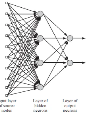
A Neural Network (NN) [12] is an algorithm designed to model the way in which the human brains perform a particular task. It consists of several units (neurons) arranged in layers connected with weights, as one can see in Figure 2.1.
Figure 2.1: Scheme of a Neural Network
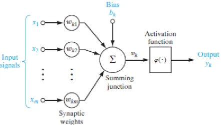
A neuron is an information-processing unit that is fundamental to the operation of a NN. The diagram of Figure 2.2 shows the basic model of a neuron. The neuron
receives a set of input signals, each of which is characterized by a weight of its own. The neuron processes the weighted inputs, usually summing them, and determines if the result surpasses a certain threshold, through the so-called activation function. The neural model also includes an externally applied bias, that has the effect of increasing or lowering the input of the activation function.
Figure 2.2: Scheme of a single neuron
There are a number of activation functions used in NN, some of them are: 1. Threshold function: it is the simplest one. Given a vectorx, it is computed as:
ϕ(x) =
1 x≥0 0 x≤0
2. Rectified Linear Unit, known as ReLU. Given a vectorx, ReLU(x) = max(0, x)
3. Sigmoid function. It is one of the most used activations functions in NN. It has the form, for a vectorx:
ϕ(x) = 1
1 + exp(−ax)
whereais the slope parameter.
Another important aspect of a Neural Network is its architecture (structure). There are three fundamentally different classes of neural architectures:
Chapter 2. DNN topology 13
1. Single-layer Feed-Forward Network. It is the simplest form of a layered net-work. We have an input layer of sources nodes that project directly onto an output layer of computational nodes.
2. Multi-layer Feed-Forward Neural Network (FNN). In this case there are one or more hidden layers (the ones that are neither the input layer nor the output layer). We use the name Multilayer perceptron (MLP) in case the FNN has only one hidden layer, and we use Deep Network (DN) when the hidden layers are more than one. By adding more layers, the network is enabled to extract higher-order statistics from its input. The lack of cycles characterises the Feed-Forward Network. We can also differentiate between a fully connected network, when every node in each layer is connected to every node in the adjacent forward one, and a partially connected network when some of the communications links are missing.
3. Recurrent Network (RNN). It distinguishes from the Feed-Forward Network NN in that it has at least one feedback loop. The presence of feedback loops has a profound impact on the learning capability of the network.
From now on we will work with Feed-Forward Deep Neural Networks with ReLU activations for all the nodes.
We introduce the following notation:
K number of layers
nk number of nodes in layerk
Wk∈Rnk×
Rnk−1 matrix of weights from layerk−1tok
bk ∈Rnk bias vector from layerk
φk activation function in layerk
Using the previous notation, and considering that for our workφk =ReLU, k =
1. . . K, the output vectorxk is defined as:
xk =ReLU(Wk−1xk−1+bk−1) =f(Wk−1, bk−1;xk−1)
We denote the transfer function byf.
The output of a FNN is computed as:
xK =fK(Wk−1, bk−1;fk−1(Wk−2, bk−2;...f1(W0, b0;x0)...)) (2.1)
A Neural Network is nothing more than a series of connections between units. The connections depend heavily on the weights. Finding the weights, which will allow the machine to predict the correct output, is one of the crucial problems in the training process. This is discussed in the following sections.
Chapter 3
Training a DNN
In this section we will present the Weights and Bias Optimization (WBO) problem for a DNN with ReLU activation function. We will suppose that the hyper-parameters, i.e. the neural architecture such us the number of neurons and layers, are already fixed, and our network training will aim at finding the weights and bias such as the given data set is mapped to our desired output values with the least error possible. We will study two different problems: regression and classification.
We introduce the WBO and some results commented in [16] and all the references therein.
3.1
The Weights and Bias Optimization Problem
Given an NN withK layers, layerkwithnknodes, if we denote byWk ∈Rnk ×
Rnk−1 andbk ∈
Rnk respectively the matrix of weights from layerk −1tok and the
bias vector from layerk, and byw={W0, . . . , WK},b={b0, . . . , bK}, the Weights
and Bias Optimization Problem is defined as follows:
minE(w,b) =
n
X
i=1
Ei(w,b) +λkwk2+λkbk2 (3.1)
whereEi(w,b) :R→R+is the loss function, assumed to be continuous, that depends
on the problem at hand, andλ≥0is assumed to be fixed. The regularization or penalty termsλkwk2andλkbk2withλ≥0are added to secure better generalization and avoid
having an over-fitting phenomena in some cases.
We observe that the problem (3.1) admits a global minimum for any λ > 0. In-deed, by definition,Ei(w,b)≥0, and, thanks to the regularization term, the objective
function is coercive, that is, for any (w0,b0)
where M = E(w0,b0)
, there exists a 15
constantRsuch that wheneverkwk,kbk ≥R, then E(w,b) > M. Hence, the levels set A = (w,b) :E(w,b)≤E(w0,b0) are all compact for every w0,b0 and the functionE admits a global minimum(w∗,b∗)such thatE(w∗,b∗)≤ E(w,b)for all
(w,b). This property may not hold if the penalty term is removed, i.e., forλ= 0. One important question to ask is whether global optimization is needed or whether local optimization is enough to solve the problem. To answer this, first we will intro-duce some results about the complexity of the problem.
3.1.1
Complexity of training a ReLU NN
Recently, some results about hardness for ReLU networks have been shown by [6]. The main results are:
Theorem 3.1.1. It is NP-hard to solve the training for a two layer ReLU NN with two ReLU nodes in the first layer and one in the last one.
Corollary 3.1.1. The training problem of a two layer ReLU NN with two nodes in the first layer and j in the last one is NP-hard, for allj ≥1.
Theorem 3.1.2. Under the assumption that the dimension of input d is a constant, there exists a poly(N) solution to the training problem of a ReLU NN with two nodes in the first layer and one in the second and last one, where N is the number of data points.
Theorem 3.1.3. Given data points{xi, yi}i = 1. . . N, then the training problem for
a ReLU NN with N nodes in the first layer and one in the second and last one has a poly(N,d) radomized algorithm, whereN is the number of data points anddis the dimension of input.
In the same line of research, [1] shows:
Theorem 3.1.4. There exists an algorithm to find a global optimum of the minimization problem to train a two layer ReLU DNN in timeO(2w(D)nwpoly(D, d, w)). Note that the running time is polynomial in the size data for fixedd, dimension of input, and fixed
w, number of nodes.
These results show that the running time of an algorithm to find the global mini-mum of a two layer ReLU DNN is exponential in the input dimension and the number of hidden nodes, and only if they are fixed the running time of the algorithm could be polynomial.
We observe the complexity of training a ReLU NN even in the easiest network architecture (shallow networks with few neurons).
Chapter 3. Training a DNN 17
However, it has been observed in practice that "most local minima yield similar performance from the generalization point of view. Furthermore, as asserted in [7], the probability of finding a bad local minimum, namely one with large training error, decreases quickly with the network size. Hence, for deep ReLU networks the effort of finding the global minimum may not be worthwhile." It has also been suggested by several authors that, because of overfitting phenomena, inaccurate weights minimiza-tion can be better than exact ones [15].
Assuming continuous differentiability of the function E, any gradient-based un-constrained method can be applied to the solution of the WBO problem (3.1). Con-sidering previous results, we will solve problem (3.1) with local-search algorithms, such as gradient methods. These methods can guarantee convergence only to station-ary points, but in practice it will probably be fully satisfactory from the generalization point of view.
We will formulate the WBO problem for two different problems: classification and regression.
3.1.2
Regression
Let us consider a feed-forward DNN with K+1 layers and ReLU activation. Given data points (x0
i, yi0) ∈ Rm ×R, i = 1. . . n, we consider the problem of finding the
weights that minimize the error function. In this case the error function is defined as: Ei(w,b) = kf(x0i)−y
0
ik
2
+λkwk2+λkbk2 (3.2) wheref(x0i) = xKi , and the regularization termλ >0is fixed.
The optimization problem is:
min n X i=1 (xKi −y0i)2+λkwk2+λkbk2 (3.3) s.t. xK i =ReLU(WK −1xK−1 i +bK −1) .. . x1 i =ReLU(W0x0i +b0) i= 1. . . n (3.4)
There are various ways of modelling the constraints of this problem. First we will study the basic scalar function:
One can reproduce a formulation for the ReLU as below. wTy+b =x−s xs ≤0 x≥0, s≥0 (3.5)
With this formulation, we separate the positive and negative part of the ReLU. WhenwTy+b≥ 0, s = 0andx=wTy+b, whilex= 0whenwTy+b <0. For us
to not work with a bilinear condition such as xs ≤ 0, one can rewrite the expression by introducing a binary activation variablez. This yields:
z = 1→x≤0 z = 0→s≤0 z ∈ {0,1} (3.6)
Using these new variables, we obtain the following WBO problem:
min n X i=1 (xKi −y0i)2+λkwk2+λkbk2 (3.7) s.t. Wk−1xK−1 i =ziKxKi −sKi .. . W0x0 i =zi0x0i −s0i i= 1. . . n (3.8) xk i ≥0, ski ≥0 zik ∈ {0,1} if zk i = 1,then xki ≤0 if zk i = 0,then ski ≤0 ∀i= 1. . . n ∀k= 1. . . K (3.9)
This reformulation may be useful in some cases, but introducing an integer variable while working with a linear objective function may not be the best idea, as a non-linear integer optimization problem is a very complex computational problem.
Another way to reformulate the ReLU function is using the hyperbolic approxima-tion:
max{t,0} ' √
t2+ε+t
2 , for some small ε >0 (3.10)
We obtain now a non-linear optimization problem without integer variables:
min
n
X
i=1
Chapter 3. Training a DNN 19 s.t. xK i = √ (WK−1xK−1 i +bK−1)2++W K−1xK−1 i +b K−1 2 .. . x1 i = √ (W0x0 i+b0)2++W0x0i+b0 2 i= 1. . . n (3.12)
3.1.3
Classification
In this case, given data points x0
i ∈ Rq, i = 1. . . n and a set of categories
yi, yi = 1. . . p,i= 1. . . n, the problem consists in finding the weights and bias which
maximize the probability of each observation being mapped to its right category. Instead of considering that the last layer consists in one single node whose value is the corresponding class, it will be ap-dimensional vector, whose maximum component will indicate to which category the data point belongs. An individual x0j would be classified correctly if(xK
j )yj >(x
K
j )k, for all k ={1. . . p}\{yj}, whereKindicates
the output layer, and the sub-index refers to the component of the output vector. We assume a random classification rule, in which an individualx0 will be assigned
to class j with probability proportional to e(xK)j, j = 1. . . p, i.e., with probability
e(xK)j
Pp
k=1e
(xK)k. Hence, the probability of correct classification of an individualx
0 in class
yis Ppe(xK)y k=1e
(xK)k.
To train the classification problem, we maximize the expected number of correctly classified individuals. Thus, the loss function for this problem is defined as:
min− n X j=1 e(xKj)yj Pp k=1e (xK j )k +λkwk 2+λkbk2 (3.13)
whereλ >0is fixed. For the formulation we use the constraints (3.12) The final formulation is given by:
min− n X j=1 e(xKj)yj Pp k=1e (xK j )k +λkwk2+λkbk2 (3.14) s.t. xKi = q (WK−1xK−1 i +bK−1) 2 ++WK−1xK−1 i +bK −1 2 .. . x1 i = q (W0x0 i+b0) 2 ++W0x0 i+b0 2 i= 1. . . n (3.15)
Instead of maximizing the expected number of correctly classified individuals, we might minimize the number of misclassified points in the data set. To do this we intro-duce a binary variablezi which yields:
zi = 1 if (xKi )yi ≤(x K i )j, j={1. . . p} \yj zi = 0 otherwise zi ∈ {0,1} i= 1. . . n (3.16) This logical implication can be converted into inequalities using the bigM method. This yields
(xKi )yj ≤zi(x
K
i )j +M(1−zi) j ={1. . . p} \yi, i= 1. . . n (3.17)
where M is a finite non-negative value long enough, so that, ifz = 0, then the con-straint would be not binding.
The final formulation in this case is given by:
min n X i=1 zi+λkwk2+λkbk2 (3.18) s.t. (3.12),(3.17) (3.19)
This alternative formulation might be used, but, as it has been commented on early, using binary variables and non-linear constraints is not the best idea. Hence, the first formulation would be used for our computational experiments.
3.2
Computational experiments
In this chapter the WBO (3.1) is applied to a given set of data points. As it has been said, the network architecture will be considered fixed, but we will study multiple structures of the NN to see which one is best suited for our problem.
As the optimization problem will be solved with local-search algorithms and in practice there will be more than one local minimum, a good way to ensure finding the solution is to apply the multi-start technique, namely, running the algorithm with different starting points. The regression and classification problem will be both ad-dressed, and will be used to solve both problems the NEOS Server, an internet-based
Chapter 3. Training a DNN 21
service for solving numerical optimization problems. The AMPL codes can be found in Annex I. The software MINOS, which is designed to solve continuous non linear programming problems, will be used to solve all the examples in this chapter.
The running time used for each example will not be presented, as we are using NEOS Server, the software and computer used to solve each example would be differ-ent, hence the different running times would not be comparable.
3.2.1
Regression Problem
We consider the problem of assessing the heating load requirement of a building, that is the energy efficiency, as a function of building parameters.
The dataset, known in the literature as Energy efficiency, was created by Angeliki Xifara and was processed by Athanasios Tsanas [18]. It can be found in [19]. It compromises 750 samples of 12 different buildings, 400 of which will be used to train the network, and 350 to test it. It contains eight attributes (x1, x2, x3, x4, x5, x6, x7, x8) and, originally, two responses (y1, y2). For our experiment, we will use one of them, y1. Predicting the second response y2 would be analogue. The aim is to train our NN to be able to predict the response using the eight factors.
These are specifically:
• x1: relative compactness • x2: surface area • x3: wall area • x4: roof area • x5: overall height • x6: orientation • x7: glazing area
• x8: glazing area distribution
• y1: heating load
Model (3.11)-(3.12) is applied to these data points.
To perform the experiments, four different network architectures will be consid-ered:
• DNN2: 1 hidden layer with 10 neurons
• DNN3: 2 hidden layers with 3 neurons each
• DNN4: 2 hidden layers with 8 neurons each
All DNNs involve an input layer with eight neurons and an output layer with one unit.
As parameters, the valuesλ= 0.01and= 10−3have been used.
Results
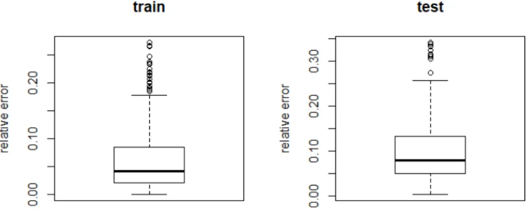
For each structure we will show the relative error for the training and testing set. The first structure that has been used is very simple. The results are shown in Fig-ure 3.1.
Figure 3.1: Performance on a 5-3-1 Neural Network
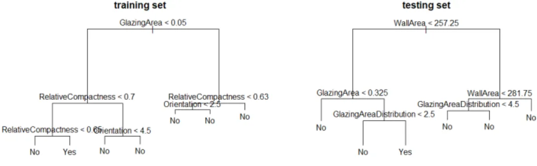
Although the network structure used was very simple, the results obtained are quite satisfactory, as the mean relative error for the training and testing set is around 5 % and 10 % respectively. One thing that must be discussed is the presence of quite some outliers, whose relative error is quite big. We have performed some experiments to identify the records yielding such errors. To do this, we have considered a classification problem in which the class was 1 or 0 whether the relative error was above or below 20 %. A classification tree [14] was run for both data sets, the training and the testing one. The results shown in Figure 3.2 show us that, although it gives us exactly which combination of factors leads to a bigger error, it is not fully clarifying, as both trees do not even coincide for both tests.
Chapter 3. Training a DNN 23
Figure 3.2: Classification tree for DNN1. Relative error above or below 20%
If we add nodes to the hidden layer, the relative error for the training set is highly reduced, but for the testing one, the results are worse than for the last structure used. While the mean relative error is similar, we found in this case a lot more dispersion, and in general worse capacity of a good prediction. Looking at the results in Figure 3.3, it seems that the model obtained is overfitted, and thus, worse prediction results are achieved.
Figure 3.3: Performance on a 8-10-1 Neural Network
Maintaining the same number of nodes as DNN1, but adding an additional layer reduces the relative error for the testing data sets, and this result interests us much more, as it means that the prediction capacity of our network has increased. The relative error for the training set does not change and this could possibly mean that, as opposed to the latter case, the model obtained is not overfitted.
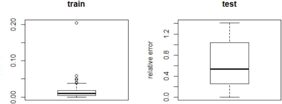
Figure 3.4: Performance on a 8-3-3-1 Neural Network
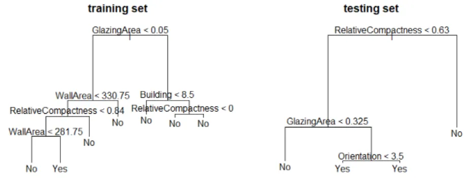
In this model, there are some outliers as well. We have performed the same ex-periment as before to identify them, and using a classification tree we have obtained the combination of attributes that make our model unsuitable for those cases, see Fig-ure 3.5. Although there are some characteristics common for some of them, the trees are all different, hence we can’t determine exactly what factors cause most errors in our model. However, one can observe that the Relative Compactness(X1) and specially the Glazing Area (X7) are the attributes that determine most the probability of having a bigger error.
Figure 3.5: Classification tree for DNN3. Relative error above or below 20%
At last we consider the largest DNN. For this one, we can clearly see an overfitted model, as shown in Figure 3.6. The error for the training set is the lowest, but for the testing set we obtain the worst results achieved at the moment. The mean relative error
Chapter 3. Training a DNN 25
for this one increases to a value of 50 %, and it reaches as far as 140 %, which gives us an impractical model.
Figure 3.6: Performance on a 8-8-8-1 Neural Network
To sum up, for this regression problem, the best architecture network to use would be DNN3. The results in this case, are fully satisfactory, as we achieve a mean relative error for the testing set of the 7 %, with little variance. This brings to light the fact that a hidden layer can increase the network ability to compute and extract high-order statistics from the input. However, it must be considered that too many parameters tend to overfit the model, as it has been proven in the last case, where increasing the number of nodes excessively makes the network completely ineffective.
3.2.2
Classification Problem
In this case we consider the problem of knowing if a specific breast cancer is benign or malignant. The dataset compromises 684 samples obtained from the University of Wisconsin Hospital. The dataset can be found in the UCI Machine Learning Datasets webpage [20]. Each sample contains 9 attributes (X1-X9) and its corresponding class (Y). These are:
1. X1: Clump Thickness: 1-10 2. X2: Uniformity of Cell Size: 1-10 3. X3: Uniformity of Cell Shape: 1-10 4. X4: Marginal Adhesion: 1-10
6. X6: Bare Nuclei: 1-10 7. X7: Bland Chromatin: 1-10 8. X8: Normal Nucleoli: 1-10 9. X9: Mitoses: 1-10
10. Y: 1 for benign, 2 for malignant
Model (3.14)-(3.15) is applied to 342 of these data points for training, while the rest of them will be used for testing.
To perform the experiments, four different NN structures will be considered:
• DNN1: 1 hidden layer with 3 neurons
• DNN2: 1 hidden layer with 10 neurons
• DNN3: 2 hidden layers with 3 neurons each
• DNN4: 2 hidden layers with 8 neurons each
All DNNs involve an input layer with nine neurons and an output layer with two units. It has also been usedλ= 0.01and= 10−3 as parameters values.
Results
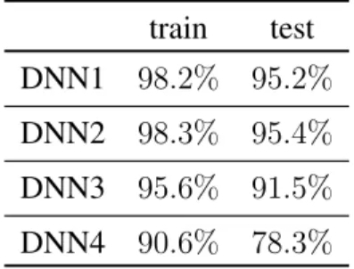
For the classification problem, the accuracy of the model is our performance mea-sure. In Figure 3.7 the percentage of correctly classified sets is shown for the train and test set using the different DNN structures.
train test DNN1 98.2% 95.2%
DNN2 98.3% 95.4%
DNN3 95.6% 91.5%
DNN4 90.6% 78.3%
Chapter 3. Training a DNN 27
As we can see, highly complicated architectures are not necessary to address this classification problem. In fact having more hidden layers would probably accomplish an over-fitted model, whose capacity of prediction would probably be reduced.
It is also worth commenting, how, when a more complicated structure was used, namely, DNN4, the solution was degenerate, that is, we found quite a number of rows and columns of the weights matrix to be null.
The results differ a little from those obtained in regression. In this case, the best architecture to model this problem is DNN2. One can observe that the results are more satisfactory for simple structures, as using DNN1 gives us already a level of accuracy quite high. The reason behind this is probably that the relations between the attributes in this case are less complex than in the regression one, hence, it is not needed a complex network to predict the outputs, and using one is only counterproductive.
Chapter 4
The inverse problem
In this chapter we consider given an already trained DNN with ReLU activation. We will investigate a 0-1 MILP model with fixed parameters, as studied in [10]. We will also describe some bound-tightening techniques to decrease the running time. These techniques have been studied in [8] and [9]. As all parameters are already fixed, this model cannot be used for training, but we will discuss alternative applications of this model, such as feature visualization and construction of adversarial examples.
4.1
A trained Deep Neural Network
Let us consider a DNN made up ofK+ 1layers, where 0 is the index of the input layer, while the last layer corresponds to the output. Each layer is composed of ni
nodes, i.e. neurons, i= 1..k, wherek is the dimension of the layer. We denote byxkj as the output value for the j-unit of layer k.
Given an input value for the Feed-Forward Network, a non-linear function is ap-plied successively from 0 to K. In this case, we will assume that this function is a
rectified linear unit, ReLU.
Letxkbe the output vector for layer k:
xk =ReLU(Wk−1xk−1+bk−1) k=1 . . . K (4.1) In this recursive description, for a real vector y, ReLU(y) = max(0, y) andwij
andbi are the weights and bias, which in this case will have fixed values.
There are various ways of modelling a given DNN, one of them leads us to a Mixed-Integer Linear Programming model, the one examined first in what follows.
4.2
Mixed-Integer Linear Formulation
To obtain a 0-1 MILP model, one needs to study the equation: x=ReLU(wTy+b)
This equation has already been studied in Chapter 3. We formulate the ReLU using the expressions (3.5) and (3.6). The logical implication of (3.6) can be converted into proper linear inequalities. One method that is widely known is the bigM method, which yields:
x≤M+(1−z) (4.2)
s≤M−z (4.3)
whereM+, M−are finite non-negative values large enough, such that−M−≤wTy+
b ≤M+.
Whenz = 1, s ≤ M−, which is not binding and x ≤ 0, that implies thatx = 0. Whenz = 0, x ≤ M+ is not binding if M+ is large enough, ands ≤ 0implies that
x=wTy+b.
Using a binary activationzk
j for each neuron and consideringzk as the vector for
each layer,k= 1. . . K, one obtains the following 0-1 MILP formulation of the DNN:
min K X k=0 ckxk+ K X k=1 γkzk (4.4) s.t. Wk−1xk−1+bk−1 =xk−sk xk j, skj ≥0 zk j ∈ {0,1} xkj ≤Mjk+(1−zjk) sk j ≤M k− j zjk k = 1. . . K, j = 1. . . nk (4.5) lk j ≤xkj ≤ukj ¯ lk j ≤skj ≤u¯kj k= 1. . . K, j = 1. . . nk (4.6)
In the (4.4)-(4.6) formulation, the objective function costsck
kandγjkare given
con-stant parameters, that can be defined according to the specific problem at hand. Con-ditions (4.5) define the ReLU output for each neuron, while conditions (4.6) impose the lower and upper bounds on xand s, fork = 0 l0
j andu0j apply to the input value
x0
j and depend on the problem at hand, while for k ≥ 1 one has lkj = ¯ljk = 0 and
Chapter 4. The inverse problem 31
4.3
Bound tightening
The efficiency of this formulation depends heavily on the size of M+ and M−
. They have to be big enough to guarantee that the constraint is inactive ifz = 1and it is not binding ifz = 0, but large big-M results in a weak LP relaxation. For this reason, we will study a way to choose a relatively small value of M.
Looking at the problem, we can see that defining tight upper-bounds will be crucial for this reason, as the smaller value ofMjk+andMjk−possible areukj andu¯kj respectively. We will study in this section different ways to obtain tighter bounds, that will automat-ically give us a smaller M value for our formulation.
Obtaining bounds using interval arithmetic
One way to obtain tighter upper and lower bounds is using interval arithmetic [13]. In the spirit of [8] and [9], one can obtain the bounds lkj, ukj for the node output xkj from the bounds of nodes from the previous layer. The outputxk
j is defined by xkj = Pnk−1 i=1 w k−1 ij x k−1 i +b k−1
j . Applying interval arithmetic we can obtain the bounds as
follows: ˜lk j = nk−1 X i=1 min(wkij−1ljk−1, wijk−1ukj−1) +bkj−1 (4.7) ˜ ukj = nk−1 X i=1 max(wkij−1ljk−1, wijk−1ukj−1) +bkj−1 (4.8) If we separate the cases wherewk
ij has a positive or negative value and using the
notationa+ = max(a,0)anda− = min(a,0), we can rewrite the equations (4.7) and
(4.8) as: ˜ ljk= nk−1 X i=1 (wij+(k−1)ljk−1+wij−(k−1)ukj−1) +bkj−1 (4.9) ˜ ukj = nk−1 X i=1 (wij+(k−1)ljk−1+wij−(k−1)ukj−1) +bkj−1 (4.10) To obtain the bounds forxkj one has to apply theReLU activation.
lkj, ukj=hmax(0,˜lkj),max(0,u˜kj)i (4.11) Following the same steps, one can define bounds forskj. If we look at our formula-tion, the variablesk
j is active whenxkj = 0and in that caseskj =−
Pnk+1 i=1 w k−1 ij x k−1 i +
ˆ lkj = nk−1 X i=1 (−w−ij(k−1)ljk−1−wij+(k−1)ukj−1)−bkj−1 (4.12) ˆ ukj = nk−1 X i=1 (−w−ij(k−1)ljk−1−wij+(k−1)ukj−1)−bkj−1 (4.13) To propagate the bounds we apply theReLU activations to the them:
¯
lkj,u¯kj
=hmax(0,˜lkj),max(0,u˜kj)i (4.14)
4.4
A Non linear reformulation
An alternative form to model indicator constraints, like ReLUs, is using Mixed Integer Non-linear Programming [3], [5]. Instead of using a linear formulation and the so-called big-M constraint, that can lead to weak continuous relaxations, we present in this section a possible non-linear, non-convex reformulation for the same model.
A 0-1 MINLP formulation
min K X k=0 nk X j=1 ckjxkj + K X k=1 nk X j=1 γjkzjk (4.15) s.t. Pnk−1 i=1 w k−1 ij x k−1 i +b k−1 j =xkj −skj xkj, skj ≥0 ¯ zjk ∈ {0,1} xkj(1−z¯jk)≤0 skjz¯kj ≤0 k = 1. . . K, j = 1. . . nk (4.16) lkj ≤xkj ≤ukj ¯ lkj ≤skj ≤u¯kj k= 1. . . K, j = 1. . . nk (4.17)4.5
Computational Experiments
We will use again the NEOS Server to solve the problems in this section. The AMPL codes can be found in Annex II. The software CPLEX, which is designed to solve mixed-integer linear programming (MILP), will be used to solve all the examples in this section.
Chapter 4. The inverse problem 33
Just as we commented on Chapter 3, the running time used for each example will not be shown, as using the NEOS Server does not assure us to have running times hat are comparable. For this reason, the bounds tightening techniques will not be used in this computational experiments.
As noted before, the model (4.4) - (4.6) is not suited for training, but we can use it to compute the best-possible input example according to some linear objective function, that will depend on the problem at hand. In this section we will apply our model to a feature visualization problem and we will build adversarial examples.
4.5.1
Feature visualization
We consider the classification problem of knowing if a specific breast cancer is benign or malignant. We will use our 0-1 MILP model to find the input examples that maximize the activationxKj of each class. HerexKj denotes de j-th node of the output layer. To solve this problem the objective function is simply:
−xKj (4.18)
wherej = 1,2depending if one wants to find the input that maximizes the first class or the second one.
We will use the trained DNN3 in Chapter 3. This DNN had 2 hidden layers with 3 neurons each, and it produced a test-set accuracy of 91.5 %. Its corresponding weights and bias were used to build our (4.4) - (4.6) model.
Results
We present in Figure 4.1 the input examples that maximize each class. max-activating input
benign (Y1) (0,0,0,10,10,0,10,0,0)
malignant (Y2) (10,0,0,0,0,10,0,0,10)
Figure 4.1: Input examples that maximizes each class
Knowing these results, one could analyse each input and conclude that those whose factors X4 (Marginal Adhesion), X5 (Single Epitheial Cell Size), and X7 (Bland Chro-matin) are more prominent, could be classified with more probability as benign, while factors X1 (Clumb Thickness), X6 (Bare Nuclei), and X9 (Mitoses) identify clearly the malignant class.
4.5.2
Adversarial Examples
In this case we will use our MILP model to simulate the role of a malicious at-tacker. We want to locate which minimal changes in the model are sufficient to trick the DNN and make a wrong classification. We will use again as illustration the breast cancer classification problem.
We are given an inputx˜0 that is classified correctly by our DNN asi(benign or
malig-nant). We want to determine the minimum distance betweenx˜0 and a similar figurex0
that it is wrongly classified asj 6=i.
To model this situation we impose that in the last layer the activation of the required wrong class is at least 20 % larger than the other activation. In our MILP model (4.4)-(4.6) we just have to add the linear constraints:
xKj ≥1.2xKi , i, j = 1,2 (4.19) In order to minimize the distance betweenx0 andx˜0 in`
1 norm, we minimize the
following objective function:
n0
X
j=1
|x0j −x˜0j| (4.20)
In order to have a linear objective, the problem is reformulated as minimizing
n0
X
j=1
dj (4.21)
where the variablesdj must satisfy:
−dj ≤x0j −x˜
0
j ≤dj, dj ≥0 j = 1. . . n0 (4.22)
This linear constraint must be also added to model (4.4)-(4.6). We will use again the trained DNN3 in Chapter 3, which had 2 hidden layers with 3 neurons each and it produced a test-set accuracy of 91.5 %. Its corresponding weights and bias were used to build our model.
Results
Considering two inputs, corresponding to the two different classes, it is shown in Figure 4.2 the minimum changes in the original input that suffice to trick the DNN and therefore it would make a wrong output. One can see that the changes are not minimal, and that there are variables more relevant than others.
It can be easily seen that the parameters that one must change in order to trick the DNN are the ones that where calculated in the last example, those who maximized
Chapter 4. The inverse problem 35
original input adversarial example Pn0
j dj
benign (2,1,1,1,2,1,3,1,1) (2,1,1,1,2,4,3,1,10) 12
malignant (6,10,10,10,8,10,7,10,7) (6,10,10,10,8,1,7,8,1) 17
Figure 4.2: Adversarial examples that trick the DNN
their correspondent output. The results are therefore very logical and expected.
We can also impose to our model other interesting constraints such as: maximum deviation for each attribute with respectx˜0 or maximum number of changed attributes
in the inputx0, as illustrated in what follows.
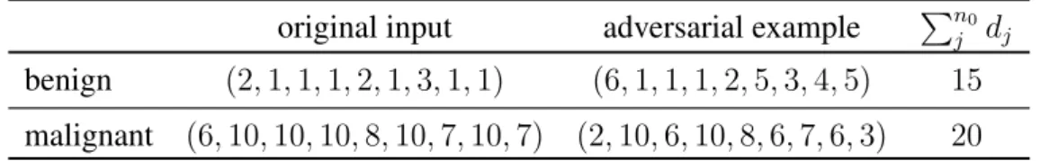
First we impose that the maximum allowable deviation for each attribute is 4. We just add to our model thatdj ≤4, j= 1. . . n0.
The results obtained in this case are:
original input adversarial example Pn0
j dj
benign (2,1,1,1,2,1,3,1,1) (6,1,1,1,2,5,3,4,5) 15
malignant (6,10,10,10,8,10,7,10,7) (2,10,6,10,8,6,7,6,3) 20
Figure 4.3: Adversarial examples that trick the DNN, maximum deviation each at-tribute:4
We can see that, imposing this constraint, the changes in the input to trick the NN increase. This is definitely a good sign, as it confirms us the reliability of the network. In fact, if we impose that the maximum allowable change must be 3 or smaller, the optimization problem turns to be infeasible, i.e. there would not be any combination of changes that could trick our network.
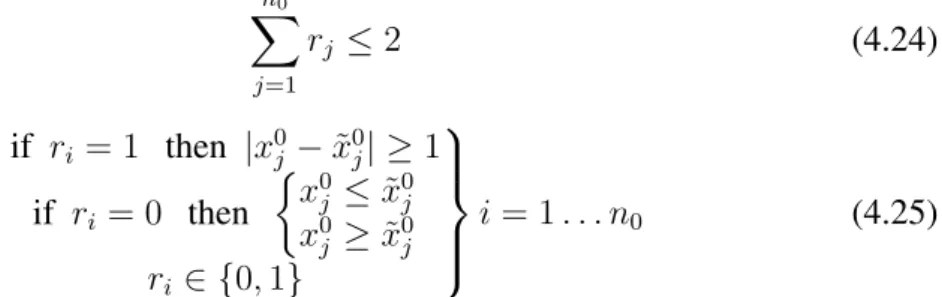
At last we add that the maximum number of modified attributes must be 2. For us to solve this we must introduce binary variablesri,i= 1. . . n0. This yields
ri = 1 if componentiis modified ri = 0 otherwise ri ∈ {0,1} i= 1. . . n0 (4.23)
Knowing that, if componentj has changed, then |x0
˜
x0
j| = 0, the following constraints must be add to our model to limit the number of
changes: n0 X j=1 rj ≤2 (4.24) if ri = 1 then |x0j −x˜0j| ≥1 if ri = 0 then x0 j ≤x˜0j x0 j ≥x˜0j ri ∈ {0,1} i= 1. . . n0 (4.25)
In order to have a linear constraint, another binary variableti,i= 1. . . n0is
intro-duced: ti = 1 if x¯0i ≥x0i ti = 0 otherwise ti ∈ {0,1} i= 1. . . n0 (4.26)
This new binary variable and a big value M, allow us to linearise the absolute value. The final new constraints added to our model are (4.24) and the following:
x0 j ≥x˜0j(1−rj) +rj(˜x0j + 1−M tj) x0 j ≤x˜0j(1−rj) +rj(˜x0j −1 +M(1−tj)) j = 1. . . n0 (4.27)
where M is a constant big enough (in this case 10 is enough).
Introducing all these factors, the new results are shown in Figure 4.4 original input adversarial example Pn0
j dj
benign (2,1,1,1,2,1,3,1,1) (2,1,1,1,2,4,3,1,10) 12
malignant (6,10,10,10,8,10,7,10,7) infeasible
-Figure 4.4: Adversarial examples that trick the DNN, maximum number of changes: 2
Imposing the maximum number of changes in only 2 nodes, the result in the first case considered (x˜0 benign) does not change, as the optimal solution without
con-straints had only changed the value of two nodes. But, in the second case, the problem turns out to be infeasible. In fact the minimum number of nodes needed to change in order to trick the DNN is 3.
Examining the results in general, one can conclude that it is generally easier to trick the network into misclassifying a benign case as malignant than the other way.
Chapter 4. The inverse problem 37
In all this examples, the running time is quite short and one obtains the optimal solution quite easily. This is because all our variables are bounded. (0 ≤ Xi ≤ 10),
and we do not use an extremely large value of M, that could probably give us quite a few problems.
Annex I. Training a DNN
In this chapter we include the AMPL codes used in Chapter 3.
Regression problem
param n; #input dim param epsi; #epsilon param K; #layers param lambda;
param nk{i in 0..K}; #number of nodes of each layer
param x0{i in 1..n, j in 1..nk[0]}; #input param y{i in 1..n}; #output
var b{k in 0..K-1, j in 1..nk[k+1]}; #bias
var W{k in 0..K-1, i in 1..nk[k+1], j in 1..nk[k]}; #weights var x{i in 1..n, k in 1..K, j in 1..nk[k]};
param erel{i in 1..n};
minimize error:
sum{i in 1..n} sum{j in 1..nk[K]} (x[i,K,j] - y[i])^2 +
lambda*(sum{k in 0..K-1} sum{i in 1..nk[k+1]} sum{j in 1..nk[k]} W[k,i,j]^2)+lambda*(sum{k in 0..K-1} sum{j in 1..nk[k+1]} b[k,j]^2); #constraints: subject to res{i in 1..n, k in 2..K, j in 1..nk[k]}: x[i,k,j]=0.5*(sqrt((sum{l in 1..nk[k-1]} W[k-1,j,l]*x[i,k-1,l]+ b[k-1,j])^2+epsi)+sum{l in 1..nk[k-1]}W[k-1,j,l]*x[i,k-1,l]+ b[k-1,j]); 39
subject to res0{i in 1..n, j in 1..nk[1]}:
x[i,1,j]=0.5*(sqrt((sum{l in 1..nk[0]} W[0,j,l]*x0[i,l]+b[0,j])^2+ epsi) + sum{l in 1..nk[0]} W[0,j,l]*x0[i,l]+b[0,j]);
Classification Problem
param n; #input dim param epsi; #epsilon param K; #layers
param nk{i in 0..K}; #nodes in each layer param lambda; #lamda
param clase{i in 1..n}; param err{i in 1..n}; param num;
param x0{i in 1..n, j in 1..nk[0]}; #input param y{i in 1..n}; #output
var b{k in 0..K-1, j in 1..nk[k+1]}; #bias
var W{k in 0..K-1, i in 1..nk[k+1], j in 1..nk[k]}; #weights var x{i in 1..n, k in 1..K, j in 1..nk[k]};
minimize error:
-sum{i in 1..n} exp(x[i,K,y[i]])/(sum{j in 1..nk[K]} exp(x[i,K,j])) + lambda*(sum{k in 0..K-1} sum{i in 1..nk[k+1]} sum{j in 1..nk[k]} W[k,i,j]^2)+lambda*(sum{k in 0..K-1}sum{j in 1..nk[k+1]} b[k,j]^2); #constraints: subject to res{i in 1..n, k in 2..K, j in 1..nk[k]}: x[i,k,j]=0.5*(sqrt((sum{l in 1..nk[k-1]} W[k-1,j,l]*x[i,k-1,l]+ b[k-1,j])^2+epsi)+sum{l in 1..nk[k-1]} W[k-1,j,l]*x[i,k-1,l]+ b[k-1,j]); subject to res0{i in 1..n, j in 1..nk[1]}: x[i,1,j]=0.5*(sqrt((sum{l in 1..nk[0]} W[0,j,l]*x0[i,l]+b[0,j])^2 +epsi) + sum{l in 1..nk[0]} W[0,j,l]*x0[i,l]+b[0,j]);
Annex II. Applications of a trained
DNN
In this chapter we include the AMPL codes used in Chapter 4.
Feature visualization
param K; #layers param nk{i in 0..K}; param W{k in 0..K-1, i in 1..nk[k+1], j in 1..nk[k]}; #weights param b{k in 0..K-1, j in 1..nk[k+1]}; #bias var x{k in 0..K, j in 1..nk[k]} >=0; var s{k in 1..K, j in 1..nk[k]} >=0; var z{k in 1..K, j in 1..nk[k]} binary; var t>=1e-2; param M1; param M2; minimize objective: -x[K,2]; #- sum{k in 0..K} sum{j in 1..nk[k]} x[k,j] ; #constraints: subject to res1{k in 1..K, j in 1..nk[k]}: x[k,j]-s[k,j]=sum{i in 1..nk[k-1]} W[k-1,j,i]*x[k-1,i]+b[k-1,j]; subject to clas1: x[K,1]+t-x[K,2]=0; subject to m1{k in 1..K, j in 1..nk[k]}: 41x[k,j]-M1*(1-z[k,j])<=0; subject to m2{k in 1..K, j in 1..nk[k]}: s[k,j]-M2*z[k,j]<=0; subject to cotas1{i in 1..nk[0]}: x[0,i]-10<=0;
Adversarial examples
param n; #number of inputs param K; #layers
param nk{i in 0..K};
param W{k in 0..K-1, i in 1..nk[k+1], j in 1..nk[k]}; #weights param b{k in 0..K-1, j in 1..nk[k+1]}; #bias
param xbar{j in 1..nk[0]}; #correct classified input param dbar; #xbar class
param d; #wrongly classified class
var x{k in 1..K, j in 1..nk[k]}>=0;
var x0{j in 1..nk[0]} integer; #wrongly classified variable var s{k in 1..K, j in 1..nk[k]} >=0;
var z{k in 1..K, j in 1..nk[k]} binary; var r{k in 1..nk[0]} binary;
var t{k in 1..nk[0]} binary;
var dis{j in 1..nk[0]} >=0; #distance
param M1; param M2; param M3; minimize objective: sum{j in 1..nk[0]} dis[j]; #constraints: subject to res1{k in 2..K, j in 1..nk[k]}: x[k,j]-s[k,j]=sum{i in 1..nk[k-1]} W[k-1,j,i]*x[k-1,i]+b[k-1,j]; subject to res2{j in 1..nk[1]}:
Chapter 4. Annex II. Applications of a trained DNN 43 x[1,j]-s[1,j]=sum{i in 1..nk[0]} W[0,j,i]*x0[i]+b[0,j]; subject to cond: x[K,d]-1.2*x[K,dbar]>=0; subject to m1{k in 1..K, j in 1..nk[k]}: x[k,j]-M1*(1-z[k,j])<=0; subject to m2{k in 1..K, j in 1..nk[k]}: s[k,j]-M2*z[k,j]<=0;
subject to resd1{j in 1..nk[0]}: #distance -dis[j]+x0[j]-xbar[j]<=0; subject to resd2{j in 1..nk[0]}: -x0[j]+xbar[j]-dis[j]<=0; subject to cotas1{j in 1..nk[0]}: x0[j]-1>=0; subject to cotas2{j in 1..nk[0]}: x0[j]-10<=0;
#subject to resd3{j in 1..nk[0]}: #max d change=4 # dis[j]<=4;
#subject to condi: #max input change=2 # sum{j in 1..nk[0]} r[j] <=2;
#subject to condi2{j in 1..nk[0]}:
# x0[j]>=xbar[j]*(1-r[j])+r[j]*(xbar[j]+1-M3*t[j]); #subject to condi3{j in 1..nk[0]}:
Bibliography
[1] Raman Arora, Amitabh Basu, Poorya Mianjy, and Anirbit Mukherjee. Under-standing Deep Neural Networks with Rectified Linear Units.arXiv e-prints, page arXiv:1611.01491, Nov 2016.
[2] P. Baldi, P. Sadowski, and D. Whiteson. Searching for exotic particles in high-energy physics with deep learning. arXiv e-prints, 5:4308, Jul 2014.
[3] Pietro Belotti, Pierre Bonami, Matteo Fischetti, Andrea Lodi, Michele Monaci, Amaya Nogales-Gómez, and Domenico Salvagnin. On handling indicator con-straints in mixed integer programming. Computational Optimization and Appli-cations, 65(3):545–566, 2016.
[4] Jacob Biamonte, Peter Wittek, Nicola Pancotti, Patrick Rebentrost, Nathan Wiebe, and Seth Lloyd. Quantum machine learning. arXiv e-prints, 549(7671):195–202, Sep 2017.
[5] Pierre Bonami, Andrea Lodi, Andrea Tramontani, and Sven Wiese. On math-ematical programming with indicator constraints. Mathematical Programming, 151(1):191–223, 2015.
[6] Digvijay Boob, Santanu S. Dey, and Guanghui Lan. Complexity of Training ReLU Neural Network. arXiv e-prints, page arXiv:1809.10787, Sep 2018. [7] Alan J. Bray and David S. Dean. Statistics of critical points of gaussian fields on
large-dimensional spaces. Phys. Rev. Lett., 98:150201, Apr 2007.
[8] Rudy Bunel, Ilker Turkaslan, Philip H. S. Torr, Pushmeet Kohli, and M. Pawan Kumar. A Unified View of Piecewise Linear Neural Network Verification. arXiv e-prints, page arXiv:1711.00455, Nov 2017.
[9] Chih-Hong Cheng, Georg Nührenberg, and Harald Ruess. Maximum resilience of artificial neural networks. Lecture Notes in Computer Science, page 251–268, 2017.
[10] Matteo Fischetti and Jason Jo. Deep neural networks and mixed integer linear optimization. Constraints, 23(3):296–309, 2018.
[11] Daniel Guest, Julian Collado, Pierre Baldi, Shih-Chieh Hsu, Gregor Urban, and Daniel Whiteson. Jet flavor classification in high-energy physics with deep neural networks. arXiv e-prints, 94(11):112002, Dec 2016.
[12] Simon Haykin. Neural Networks: A Comprehensive Foundation. Prentice Hall, 1999.
[13] Timothy J. Hickey, Qun Ju, and M. H. van Emden. Interval arithmetic: From principles to implementation. J. ACM, 48:1038–1068, 2001.
[14] Gareth James, Daniela Witten, Trevor Hastie, and Robert Tibshirani. Tree-Based Methods, pages 303–335. Springer New York, New York, NY, 2013.
[15] Yann A. LeCun, Léon Bottou, Genevieve B. Orr, and Klaus-Robert Müller. Ef-ficient BackProp, pages 9–48. Springer Berlin Heidelberg, Berlin, Heidelberg, 2012.
[16] Laura Palagi. Global optimization issues in deep network regression: an overview. Journal of Global Optimization, 73(2):239–277, 2019.
[17] Masato Shirasaki, Naoki Yoshida, and Shiro Ikeda. Denoising Weak Lensing Mass Maps with Deep Learning. arXiv e-prints, page arXiv:1812.05781, Dec 2018.
[18] Athanasios Tsanas and Angeliki Xifara. Accurate quantitative estimation of en-ergy performance of residential buildings using statistical machine learning tools.
Energy and Buildings, 49:560 – 567, 2012.
[19] Athanasios Tsanas and Angeliki Xifara. UCI machine learning
repos-itory. https://archive.ics.uci.edu/ml/datasets/Energy+
efficiency, 2012.
[20] W. H. Wolberg. UCI machine learning repository. https://archive. ics.uci.edu/ml/datasets/Breast+Cancer+Wisconsin+