Some pages of this thesis may have been removed for copyright restrictions.
If you have discovered material in Aston Research Explorer which is unlawful e.g. breaches
copyright, (either yours or that of a third party) or any other law, including but not limited to
those relating to patent, trademark, confidentiality, data protection, obscenity, defamation,
libel, then please read our Takedown policy and contact the service immediately
A deterministic inference framework for
discrete nonparametric latent variable models
Learning complex probabilistic models with simple algorithms
Yordan P. Raykov
Doctor of Philosophy
ASTON UNIVERSITY
January 2017
©Yordan P. Raykov, 2017 asserts his moral right to be identified as the author of this thesis This copy of the thesis has been supplied on condition that anyone who consults it is understood to recognize that its copyright rests with its author and that no quotation from the thesis and no information
Aston University
A deterministic inference framework for discrete
nonparametric latent variable models
Learning complex probabilistic models with simple algorithms
Yordan P. Raykov
Doctor of Philosophy, 2017Abstract
Latent variable models provide a powerful framework for describing complex data by capturing its struc-ture with a combination of more compact unobserved variables. The Bayesian approach to statistical latent models additionally provides a consistent and principled framework for dealing with uncertainty inherent in the data described with our model. However, in most Bayesian latent variable models we face the limitation that the number of unobserved variables has to be specified a priori. With the increasingly larger and more complex data problems such parametric models fail to make most out of the data available. Any increase in data passed into the model only affects the accuracy of the inferred posteriors and models fail to adapt to adequately capture new arising structure. Flexible Bayesian nonparametric models can mitigate such challenges and allow the learn arbitrarily complex representations given enough data is provided. However, their applications are restricted to applications in which computational resources are plentiful because of the exhaustive sampling methods they require for inference.
At the same time we see that in practice despite the large variety of flexible models available, simple algorithms such asK-means or Viterbi algorithm remain the preferred tool for most real world applications. This has motivated us in this thesis to borrow the flexibility provided by Bayesian nonparametric models, but to derive easy to use, scalable techniques which can be applied to large data problems and can be ran on resource constraint embedded hardware.
We propose nonparametric model-based clustering algorithms nearly as simple as K-means which over-come most of its challenges and can infer the number of clusters from the data. Their potential is demon-strated for many different scenarios and applications such as phenotyping Parkinson and Parkisonism related conditions in an unsupervised way. With few simple steps we derive a related approach for nonparametric analysis on longitudinal data which converges few orders of magnitude faster than current available sampling methods. The framework is extended to efficient inference in nonparametric sequential models where exam-ple applications can be behaviour extraction and DNA sequencing. We demonstrate that our methods could be easily extended to allow for flexible online learning in a realistic setup using severely limited computa-tional resources. We develop a system capable of inferring online nonparametric hidden Markov models from streaming data using only embedded hardware. This allowed us to develop occupancy estimation technology using only a simple motion sensor.
Acknowledgments
First, I would like to express my sincere gratitude to my supervisor Max Little. During the last three years, he has provided me with unparalleled training environment. I have truly enjoyed our thought provoking group meetings and I have learned more from them than from any book I have read or any class I have taken. Most of all I thank him for his passion and enthusiasm for research which has set an example for me to follow and has sweetened the countless efforts put towards completing this work.
I would also like to thank Alexis Boukouvalas for his mentorship, encouragement, patience and support. He has had a great input on many of the ideas included in this thesis and I can safely say that without him the PhD journey would not have been nearly as much fun as it was.
I am extremely grateful to Emre Ozer for the wonderful time I had being a part of his team in ARM Research Cambridge. He has given a great twist to my research focus and has helped me discover great deal of problems I wish I could solve in future.
I also feel lucky for being a part of the Nonlinearity and Complexity Research Group in Aston whose staff and students create a wonderful and stimulating research environment. Special thanks to David Saad, David Lowe and Ian Nabney for their valuable feedback on the work presented in this thesis. I also would like to thank John E Smith for honouring me with an award for my work towards this thesis.
My research has really benefited from the knowledge I gained during all the workshops, conferences and summers schools I visited. There I was amazed with how generous leaders in the field are with their time and knowledge. Short discussions with Erik Sudderth, Jim Griffin, Michael Jordan and Francois Caron have potentially saved years of my time trying to understand some of the issues related to Bayesian nonparametrics. I owe a great debt to Peter for helping me fight the English grammar which is an old enemy of mine. I also really appreciate Reham’s efforts on proofing my thesis. And I thank Bilyan for being the first reader of my first paper.
A big thanks to all of my friends at home and across the world, for being always ready to distract me. Better not to mention names as I am bound to miss someone.
I just have to thank Victoria for all of her support and patience in the last years. And last but certainly not least I owe the world to my mother for always being there for me. I also cannot overlook the impact she had on the contributions of this thesis because nothing makes you understand a subject, like having to explain it to your mother.
Contents
1 Introduction 12
1.1 Motivation . . . 12
1.2 Contributions . . . 16
1.3 Thesis organization . . . 19
2 Discrete latent variable models and inference 21 2.1 TheK-means algorithm . . . 21
2.2 Mixture models . . . 25
2.3 The Bayesian framework . . . 26
2.3.1 Bayesian mixture models . . . 26
2.3.2 Gibbs sampling . . . 29
2.3.3 Variational Bayes inference . . . 30
2.3.4 Iterated conditional modes . . . 32
2.4 Marginalization . . . 33
2.5 The Dirichlet process . . . 34
2.5.1 Definition . . . 35
2.5.2 Constructions . . . 36
2.5.3 Pitman-Yor generalization . . . 39
2.5.4 Dirichlet process mixture models . . . 40
2.6 Overview of the relations between inference algorithms . . . 42
3 Simple deterministic inference for mixture models 45 3.1 Introduction. . . 45
3.2 Small variance asymptotics . . . 46
3.2.1 Probabilistic interpretation ofK-means . . . 46
3.2.2 K-means with reinforcement . . . 47
3.2.3 Overview . . . 48
3.3 Rao-Blackwellization in mixture models . . . 49
3.4 Collapsed K-means and collapsed MAP-GMM . . . 52
3.5 Comparison on synthetic data . . . 53
3.6 Nonparametric clustering alternatives . . . 55
3.6.1 Gibbs sampling for DPMM . . . 55
3.7 Deterministic inference for Dirichlet process mixtures. . . 57
3.7.1 Variational inference for DPMMs . . . 57
3.8 Iterative maximum-a-posteriori inference . . . 62
3.8.1 Collapsed MAP-DPMM algorithm . . . 62
3.8.2 The MAP-DPMM algorithm . . . 64
3.8.3 Out-of-sample prediction . . . 65
3.8.4 Analysis of iterative MAP for DPMM . . . 66
3.9 DPMM experiments . . . 67
3.9.1 UCI experiment . . . 67
3.9.2 Synthetic CRP parameter estimation. . . 71
3.10 Example applications of MAP-DPMM algorithms . . . 73
3.10.1 Sub-typing of parkinsonism and Parkinson’s disease . . . 73
3.10.2 Application of MAP-DPMM to semiparametric mixed effect models . . . 76
3.11 Discussion . . . 78
4 Deterministic inference and analysis of HDP mixtures 79 4.1 Introduction. . . 79
4.2 Motivation . . . 79
4.3 Hierarchical Dirichlet process . . . 80
4.3.1 Stick-breaking construction for the HDP . . . 80
4.3.2 Chinese restaurant franchise. . . 81
4.3.3 Gibbs sampling for HDP mixture models . . . 82
4.4 Deterministic inference for HDPs . . . 87
4.4.1 SVA inference for HDP mixtures . . . 88
4.4.2 Iterative maximum a-posteriori inference. . . 90
4.5 Synthetic study . . . 92
4.6 Discussion . . . 93
5 Model-based nonparametric analysis of sequential data 94 5.1 Introduction. . . 94
5.2 Hidden Markov models . . . 95
5.3 Nonparametric Bayesian HMM . . . 98
5.3.1 Gibbs sampling methods for the HDP-HMM . . . 99
5.4 Deterministic methods . . . 104
5.4.1 SVA analysis for HDP-HMM . . . 105
5.4.2 Iterative MAP inference for iHMM . . . 107
5.5 Applications. . . 111
5.5.1 Genomic hybridization and DNA copy number variation . . . 111
5.5.2 Behaviour extraction from accelerometer data . . . 113
5.6 Discussion . . . 115
6 Occupancy estimation using nonparametric HMMs 116 6.1 Introduction. . . 116
6.1.1 Motivation . . . 116
6.1.2 Challenges of human occupancy counting with a single PIR sensor . . . 117
6.1.3 Related work . . . 117
6.2.1 Collection devices . . . 118
6.2.2 Data collection . . . 119
6.2.3 Sensor data description . . . 120
6.3 Laplace modeling . . . 121
6.3.1 Regression component . . . 121
6.3.2 Time window duration . . . 122
6.4 Extracting behaviour from PIR data . . . 123
6.5 System overview . . . 125
6.6 System evaluation . . . 125
6.6.1 Fewer than 8 occupants . . . 126
6.6.2 At least 8 occupants . . . 127
6.7 Computational efficiency . . . 127
6.7.1 Choice of inference algorithm . . . 127
6.7.2 Resource evaluation . . . 129 6.8 Future work . . . 131 6.9 Discussion . . . 132 7 Conclusion 133 7.1 Summary . . . 133 7.2 Future directions . . . 134
7.2.1 Unsupervised behaviour modeling . . . 135
7.2.2 Real time learning . . . 135
7.2.3 Parallel iterative MAP methods. . . 136
A Hyper parameters updates for exponential family conjugate pairs 147 B Implementation practicalities 152 B.1 Randomized restarts . . . 152
B.2 Obtaining cluster centroids . . . 153
C Out-of-sample predictions 154
D Missing data 155
E Estimating the model hyper parameters(θ0, N0) 156
F Bregman divergences 158
G DP-meansλ parameter binary search 159
H Gibbs sampling for DPMM (spherical Gaussian) 160
I Fully collapsed CRF-based Gibbs sampler 162
List of Figures
1.1 Clustering spherical Gaussian data with varying density . . . 13
1.2 Clustering spherical Gaussian data with varying spread . . . 14
1.3 Clustering well-separated elliptical data withK-means and MAP-DP. . . 15
1.4 Clustering spherical Gaussian data withK-means and MAP-DP . . . 17
1.5 Clustering trivial elliptical Gaussian data withK-means and MAP-DP. . . 18
1.6 Clustering challenging Gaussian data with K-means and MAP-DP . . . 19
2.1 Probabilistic graphical model of the Bayesian mixture model . . . 28
2.2 Illustration of the Chinese Restaurant Process . . . 39
2.3 Synthetically generated data from DPMM . . . 42
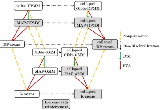
2.4 Different approaches to inference in parametric and nonparametric mixture models.. . . 43
2.5 Different approaches to inference in parametric and nonparametric hidden Markov models. . 44
3.1 Association chart of SVA, ICM and Gibbs sampling . . . 49
3.2 Probabilistic graphical model of the collapsed Bayesian mixture model . . . 51
3.3 Density of the Student-t distribution with varying degrees of freedom. . . 68
3.4 CRP mixture experiment . . . 72
3.5 Identified cluster for the ELSA longitudinal data. . . 77
4.1 Illustrating the hierarchical Dirichlet process (HDP) . . . 82
4.2 Graphical model of the HDP mixture. . . 83
4.3 Four of the synthetic data sets used for HDP experiments . . . 93
5.1 Graphical model for the Bayesian HMM. . . 95
5.2 Convergence of Gibbs and beam samplers for HDP-HMM . . . 100
5.3 Reconstructing Gaussian HMM data with asymp-iHMM . . . 107
5.4 Convergence of MCMC and ’nearly’ iterative MAP methods . . . 109
5.5 Reconstructing Gaussian HMM data with MAP methods . . . 111
5.6 MAP-iHMM applied for identification of DNA copy number regimes . . . 112
5.7 Distribution of accelerometer output from the gait for different tests. . . 114
5.8 Data quality control using MAP-iHMM . . . 114
6.1 Collecting PIR data with embedded hardware . . . 119
6.2 Example of training enviroment . . . 119
6.3 Comparison of the PIR sensor output for occupied and for empty enviroment. . . 120
6.5 Modelling occupancy with Laplace distribution . . . 121
6.6 Effect of window duration on estimated Laplace paramters. . . 123
6.7 Illustration of iHMM applied to PIR data . . . 124
6.8 Architecture of a novel occupancy estimation system.. . . 125
6.9 Box plots of extimated Laplace parameters . . . 127
6.10 Box plots of Laplace parameters after segmentation. . . 128
List of Tables
3.1 Clustering performance of MAP,K-means, E-M and Gibbs on synthetic data . . . 54
3.2 Iterations to convergence of MAP,K-means, E-M and Gibbs on synthetic data . . . 54
3.3 Clustering performance of DPMM inference techniques for the wine dataset from the UCI machine learning repository . . . 69
3.4 Clustering performance of DPMM inference techniques measured for the iris dataset from the UCI machine learning repository . . . 69
3.5 Clustering performance of DPMM inference techniques measured for the breast cancer dataset from the UCI machine learning repository . . . 69
3.6 Clustering performance of DPMM inference techniques measured for the soybean dataset from the UCI machine learning repository . . . 70
3.7 Clustering performance of DPMM inference techniques measured for the Pima dataset from the UCI machine learning repository . . . 70
3.8 Clustering performance of collapsed MAP-DPMM and collapsed Gibbs-DPMM sampling in-ference applied to Gaussian DPMM with complete covariances: UCI datasets . . . 71
3.9 Performance of collapsed Gibbs-DPMM, collapsed MAP-DPMM, DP-means and VB-DPMM inference methods used for clustering synthethic DPMM distributed data . . . 72
3.10 Significant features of parkinsonism from the PostCEPT/PD-DOC clinical reference data across clusters (groups) obtained using collapsed MAP-DPMM . . . 74
3.11 Significant likert features of parkinsonism from the PostCEPT/PD-DOC clinical reference data across clusters obtained using collapsed MAP-DPMM . . . 74
3.12 Cross-validated, average held-out likelihood for two models. . . 77
4.1 Comparison of SVA and MAP methods applied to HDP mixture . . . 92
5.1 Comparison between MAP and MCMC methods for HDP-HMM . . . 111
6.1 Accuracy of the estimated occupancy for up to 7 present. . . 126
6.2 Accuracy of the estimated occupancy for more than 8 present . . . 126
6.3 Efficiency of various iHMM inference methods for the task of occupancy estimation . . . 128
6.4 Specification of the MCUs. . . 130
6.5 Computation time and memory consumption of the system ran on difference MCUs . . . 130
6.6 Power consumption and battery lifetime . . . 130
J.1 Binomial features PD-DOC dataset. . . 165
J.2 Binary features PD-DOC dataset . . . 166
Chapter 1
Introduction
1.1
Motivation
The rapid increase in the capability of automatic data acquisition and storage is providing striking potential for innovation in science and technology. However, extracting meaningful information from complex, ever-growing data sources poses new challenges. This motivates the development of automated yet principled ways to discover structure in data. The key information of interest is often obscured behind redundancy and noise, therefore designing a plausible and statistical (or mathematical) model becomes challenging. Complex data models can be expressed in more tractable form if we instead model them using a combination of simpler components: for example consider the distribution of some data modeled with the joint distribution over an extended space consisting of both the observed variables and somelatent variables. Latent variables describe some unobserved structure in the data the type of which we define through a set of encoded assumptions inherent to our model. For example, based on what type of latent variables we assume, latent variable models can be separated into two classes: discrete and continuous latent models.
Broadly speaking, continuous latent variable models are useful for problems where data lies close to a manifold of much lower dimensionality. By using continuous latent variables, we can express inherent unobserved structure (considering it does exist) in the data with significantly fewer latent variables and therefore these latent variable models play a key role in the statistical formulation of manydimensionality reductiontechniques. Many widely-used pattern recognition techniques can be understood in that framework: probabilisticprinciple component analysis(PCA) (Tipping & Bishop,1999;Roweis,1998), the Kalman filter and others. In addition, asTipping & Bishop(1999) have pointed out, many non-probabilistic methods can be well understood as a restricted case of a continuous variable model: independent component analysis and
factor analysisfor exampleSpearman(1904) which describe variability among observed, correlated variables. By contrast, discrete latent variable models assume discreteness in the unobserved space. This discreteness naturally implies that random draws from this space have a finite probability of repetition which is one reason why discrete latent models are widely used to express inherent groupings and similarities that underlie the data. They have played a key role in the probabilistic formulation of clustering techniques. However, computationally inferring (learning) such models from the data is a lot more challenging than for continuous latent variable models and in its full generality clustering implies a combinatorial (NP-hard) problem. This often restricts the application of discrete latent models to applications in which computational resources and time for inference is plentiful.
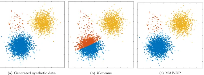
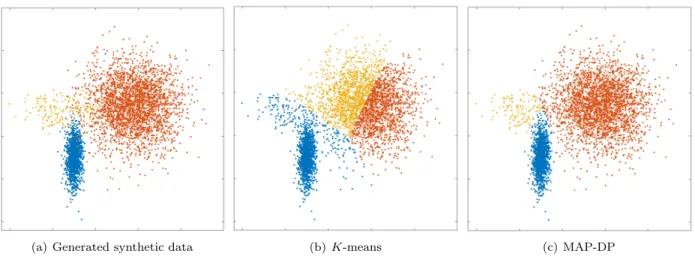
(a) Generated synthetic data (b)K-means (c) MAP-DP
Figure 1.1: Clustering performed byK-means and MAP-DP for spherical, synthetic Gaussian data. Cluster radii are equal and clusters are well-separated, but the data is unequally distributed across clusters: 69% of the data is in the blue cluster, 29% in the yellow, 2% is orange. K-means fails to find a meaningful solution, because, unlike MAP-DP, it cannot adapt to different cluster densities, even when the clusters are spherical, have equal radii and are well-separated.
discrete latent variable models. To allow for more in-depth analysis of the techniques introduced in this thesis, we will focus only on a few models which are foundational models in the field of machine learning. This will allow us to make more explicit the benefits of the proposed framework and its specific applications without having to tackle the full complexity of the overwhelmingly rich class of discrete latent variable models. However, we note that a lot of the issues we discuss here can be extrapolated to more complex and elaborate models and therefore this should be viewed as a starting point for future work in this direction.
Optimizing the efficiency of our inference procedures is not enough on its own to handle the steady growth both in terms of size and complexity of data problems that we find ourselves facing in recent years. The striking increases in the amount of data available for statistical analysis suggests a need to also change the statistical models we use. Restrictive assumptions about the structure and the complexity of a model are less likely to hold and harder to define for such situations This introduces the need for more adaptableBayesian nonparametric (BNP) models which can be used to relax such restrictions. We cannot fully appreciate the advantages that such models bring without first formally specifying the statistical and mathematical problem ofmodel selection.
Model selection Determining the structure underlying some set of observations often translates to the problem of learning a mathematical model that can accurately predict those observations. In the case of probabilistic models, we often specify the particular model and we search through a set of parameter values in the model, so that the model best explains the observations according to some criteria. This criteria is designed to indicate the generalization of a model, or how well the model describes the population of the data rather than just the observed sample. Models that are too simpleunderfit the data and fail to capture all of the inherent structure in it; models which are too complexoverfit suggesting structure for which there is insufficient evidence. For example, in the case of clustering an underfitted model would fail to discover all of the distinct clusters in the data where an overfitted model would suggest more clusters than there actually are.
A natural way to design models that are resilient to overfitting and directly enable adequate model selection is to adopt the Bayesian formalism. The Bayesian treatment to probabilistic models views all model
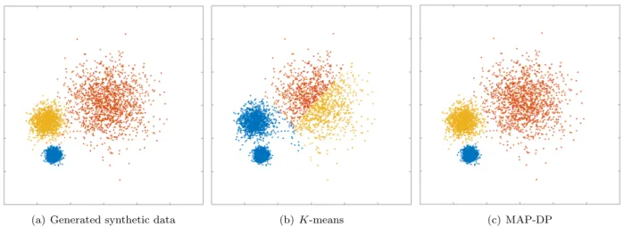
(a) Generated synthetic data (b)K-means (c) MAP-DP
Figure 1.2: Clustering performed by K-means and MAP-DP for spherical, synthetic Gaussian data, with unequal cluster radii and density. The clusters are well-separated. Data is equally distributed across clusters. Here, unlike MAP-DP, K-means fails to find the correct clustering. Instead, it splits the data into three equal-volume regions because it is insensitive to the differing cluster density. Different colours indicate the different clusters.
parameters as random variables. The distributions that specify them are calledprior distributions and they provide additional control over the behaviour of the assumed model. Model selection and model comparison can be directly performed in Bayesian models by computing themarginal likelihoodof the model. Specifically, in latent variable models the marginal likelihood is computed by taking the complete data likelihood function and integrating out the latent variables. The model which has the highest marginal likelihood is the model that best describes the data and provides the optimal fit. There are many other widely techniques for assessing the quality of fit of a model such as cross-validation, bootstraping, regularization or Bayes factors, to name a few. However, in the framework of probabilistic models many involve additional ad-hoc (heuristic) assumptions to the existing model which are not necessarily justified nor well understood. By contrast, the Bayesian paradigm addresses the specification of the model and the problem of overfitting at the same time (Bishop,2013). This often makes Bayesian models more forgiving to differences between the specification of the model and the observed data.
Now that we have defined the problem of model selection and the Bayesian approach to solving it, we can go back to specifying what we mean by BNP models in the context of latent variable models. A large class of probabilistic models (Bayesian and non-Bayesian) can be classed asparametric. Such models require the specification and choice of the number of model parameters: this is often an effective measure its complexity. In discrete latent variable models, this usually means that parametric models fix the domain of the latent variables; for example in clustering this implies fixing the number of clusters that can be found. BNP models relax this assumption allowing the model to adapt its complexity depending upon the data on which it is trained . The domain of the latent variables is defined as infinite meaning that the complexity of the unobserved structure can grow and adapt based on the evidence.
To give some specific examples, one of the most popular discrete latent variable models is theGaussian mixture model (GMM) which is formally defined in Chapter 2. The GMM models the complete dataset with a mixture of Gaussian distributions which can express complex data distributions using a combination of simple Gaussians. The unobserved variables here indicate which particular Gaussian best describes each specific point from the data. In the parametric setting the numberK of Gaussian distributions forming the likelihood of the GMM needs to be specified by design and it remains unchanged despite the size or structure
of the data . The BNP extension of the GMM (which we also define formally in Chapter2) uses as many Gaussian distributions as considered sufficient according to the model likelihood. That is, the nonparametric nature of the model aims to keep it from underfitting and the Bayesian nature of the model makes it resilient to overfitting (Hjortet al.,2010).
The problem of choosingKin a GMM has also been widely addressed outside of the Bayesian paradigmby the use of differentregularization criteria: Bayesian information criterion (BIC)(Pelleget al.,2000); mini-mum description length (MDL)(Bischofet al.,1999);deviance information criterion (DIC)(Gaoet al.,2011) to name a few. Typically a parametric model, like the GMM is fitted for different values ofKand a regular-ization criterion is used to choose the value ofK that provides the best overall fit of the model. This means repeating our inference algorithm multiple times to exhaustively search the space ofK and also relying on additional assumptions about the model which are inherent to the reguralizer but not part of the model itself1.
Unfortunately, in practice the flexibility and expressive power granted by BNP models (and often also of parametric models) carries a heavy computational price because they require computationally intensive inference methods such as Markov chain Monte Carlo sampling techniques (Hastings,1970;Geman & Geman,
1984;Chib & Greenberg,1995;Neal,2000,2003;Van Gaelet al.,2008). This is an emerging problem because we more and more often face the following situations: problems with large-scale datasets; “embedded” applications such asInternet of Things (IoT) devices where computation needs to be performed in real-time and countless applications (for example, digital signal processing; ubiquitous computing ) where computation needs to be executed on resource-constrained hardware. We are witnessing the end ofMoore’s law (Schaller,
1997;Kish,2002;Colwell,2013) which has dominated the way we think about computing and computational algorithms over the last 50 years2. Thus, there is the increasingly pressing need for approaches to inference that are not only accurate but also use minimal computational effort (Bousquet & Bottou, 2008).
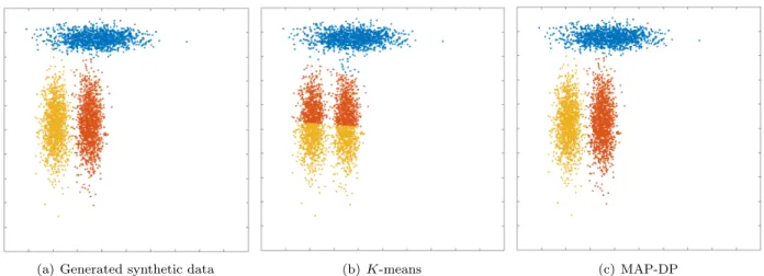
(a) Generated synthetic data (b)K-means (c) MAP-DP
Figure 1.3: Clustering solution obtained by K-means and MAP-DP for synthetic elliptical Gaussian data. All clusters share exactly the same volume and density, but one is rotated relative to the others. There is no appreciable overlap. K-means fails because the objective function which it attempts to minimize measures the true clustering solution as worse than the manifestly poor solution shown here.
1We demonstrate many of the disadvantages of regularization techniques applied to GMM andK-means clustering algorithm
in (Raykovet al.,2016c).
2Moore’s law refers to an observation made by Intel co-founder Gordon Moore in 1965. Moore’s law predicts that the number
of transistors per square inch on integrated circuits would double every year into the foreseeable future. In 1975 Gordan Moore revisited his forecast to doubling every two years. This forecast has been true for decades and has been used as an assurance for exponential grow in the computational and memory capabilities of all computational hardware.
Some of the most widely-used machine learning techniques remain deterministic algorithms such as K -means clustering (Section2.1) and it can be very helpful to look at the relationship between such techniques and discrete latent variable models; in particular how such deterministic algorithms can be derived as re-stricted inference algorithms for probabilistic models. In the case ofK-means, we can understand the general assumptions it places on the data by looking at its relation to the GMM and testing it on synthetic GMM data: K-means implies shared cluster covariance across all clusters (see Figure1.2); equal density clusters (see Figure1.1); spherical cluster geometry (see Figure1.3); known, fixed K and lack of robustness to even trivial outliers (see Figure1.4). Each of those pitfalls arises from placing certain assumptions on the related underlying GMM. Similar argument can be made for the BNP extension ofK-means -- the DP-means al-gorithm (Kulis & Jordan, 2011) and its relation to the Dirichlet process mixture model (Section 2.5.4). In fact K-means, DP-means and many other algorithms can be seen as deterministic algorithms for inference in latent variable models after applyingsmall variance asymptotics (SVA) assumptions(see Section3.2).
The reason we consider the probabilistic generalization of such techniques is so that we can revisit some of the assumptions we place on probabilistic models in our search for efficient, fast and flexible inference algorithms. We try to rigorously follow the trade-off between flexibility of the inference method and its computational efficiency(in terms of both computational speed and memory requirements). Towards this end, we map this trade-off for some of the most popular inference algorithms in the case of widely-used discrete latent variable models (such as mixture models and hidden Markov models) and their BNP extensions. We make an attempt to extend the applications for BNP models by proposing aniterative MAP (Maximum a posteriori) framework for flexible deterministic inference which can process large datasets and can operate on resource-constraint hardware, while not changing the structure of the underlying model.
Other ubiquitous methods for efficient inference in BNP models rely onvariational Bayes (VB) approxi-mations (Blei & Jordan,2006;Tehet al.,2007;Brodericket al.,2013b;Fotiet al.,2014;Hughes & Sudderth,
2013) which we discuss throughout the chapters of this thesis. Typically, VB methods are a lot harder to derive than similar iterative MAP algorithms and require additional assumptions about a model in order to make inference feasible at all.
1.2
Contributions
After more than 50 years, theK-means algorithm remains the preferred clustering tool for most real world applications (Berkhin,2006). In this thesis we study algorithms such asK-means from a probabilistic vantage point: as a restricted (SVA) case of a latent discrete probabilistic model. From this probabilistic view we can better – and more rigorously – understand the assumptions inherent with widely-used clustering methods and explore how each of those assumptions influences the flexibility, the simplicity and the usefulness of the corresponding clustering method. This sets a general framework for us to derive simple model-based algorithms, which at the cost of just slight departure from existing algorithms inherit greater flexibility and many useful statistical properties. The resulting contributions in this thesis are listed below:
We derive a modified version of K-means: collapsed K-means which is as conceptually simple, but is more robust to changes in initialization of the parameters, and is less likely to converge to a poor local solution than the originalK-means. A novelK-means with reinforcement algorithm is proposed which overcomes the implicit assumption ofK-means that data is shared equally across theK clusters.
In contrast to methods obtained using SVA assumptions to probability models, we propose an iterative,
(a) Generated synthetic data (b)K-means (c) MAP-DP
(d) Generated data (zoomed) (e)K-means (zoomed) (f) MAP-DP (zoomed)
Figure 1.4: Clustering performed by K-means and MAP-DP for spherical, synthetic Gaussian data, with outliers. All clusters have the same radii and density. There are two outlier groups with two outliers in each group. K-means fails to find a good solution where MAP-DP succeeds; this is becauseK-means puts some of the outliers in a separate cluster, thus inappropriately using up one of theK= 3 clusters. This happens even if all the clusters are spherical, equal radii and well-separated.
complex than traditional algorithms such as K-means. Some specific applications of greedy MAP have already been studied in different domains (Bertolettiet al.,2015;Besag,1986). However, here we formalize this framework and study its potential applied to different constructions of popular parametric and BNP discrete latent variable models. We systematically demonstrate the practical and conceptual advantages of iterative MAP compared to more restrictive SVA methods (Broderick et al., 2013a) for inference in BNP models.
We derive deterministic methods for inference in the Dirichlet process mixture model (DPMM): the
MAP-DPMM and the collapsedMAP-DPMM (Raykovet al.,2016c) algorithms which can be used for both approximate inference or simple nonparametric clustering algorithms which learn the number of clusters from the data. We evaluate the MAP-DPMM methods on benchmark and synthetic datasets and further compare them to both standard parametric and nonparametric clustering alternatives. We demonstrate applications of these novel methods for discovering phenotypes of Parkinson’s disease from a rich patient dataset and for nonparametric analysis of longitudinal health data.
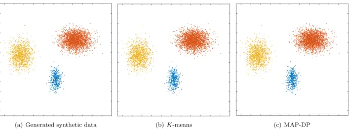
(a) Generated synthetic data (b)K-means (c) MAP-DP
Figure 1.5: Clustering solution obtained by K-means and MAP-DP for synthetic elliptical Gaussian data. The clusters are trivially well-separated, and even though they have different densities (12% of the data is blue, 28% yellow cluster, 60% orange) and elliptical cluster geometries, K-means produces a near-perfect clustering, as with MAP-DP. This shows thatK-means can in some instances work when the clusters are not equal radii with shared densities, but only when the clusters are so well-separated that the clustering can be trivially performed by eye.
applications for it as a clustering model for the standard clustering problem of data with mixed contin-uous and categorical data types. The different constructions of the HDP are conceptually contrasted and a novel deterministic clustering method, MAP-HDP,is proposed which outperforms the existing SVA alternative.
Two novel nonparametric algorithms for analysis of sequential data are proposed which we call MAP-iHMM (Raykovet al.,2015a,2016b) anddynamic MAP-iHMM. The dynamic MAP-iHMM can be seen as a nonparametric extension of the classicalViterbi algorithm for inference in hidden Markov models (HMMs). We demonstrate the applicability of MAP-iHMM and dynamic MAP-iHMM to some synthetic and real world examples, where MAP methods reach local clustering solutions orders of magnitude faster than current MCMC methods. Applications include a problem in genomic hybridization and an automated quality control for the analysis of accelerometer data collected during a walking test using a smartphone.
A novel study is performed on the challenging problem of predicting room occupancy head count using a single passive infrared (PIR) sensor (Raykovet al.,2016a). A state-of-the art system is proposed which can provide occupancy estimates every 30 seconds; the estimates are typically within +1/-1 individual of the true number of occupants. We demonstrate how, using MAP-iHMM, the whole system can be sufficiently optimized to allow it to work and segment data directly onto a highly resource-constrained microcontroller board. The loss in accuracy of the system when segmentation is done using MAP-iHMM compared to more expensive MCMC methods is negligible in practice, but this optimization allows the whole system to be deployed as a self-contained product without the need for expensive supporting computational hardware.
(a) Generated synthetic data (b)K-means (c) MAP-DP
Figure 1.6: Clustering solution obtained by K-means and MAP-DP for overlapping, synthetic elliptical Gaussian data. All clusters have different elliptical covariances, and the data is unequally distributed across different clusters (30% blue cluster, 5% yellow cluster, 65% orange). The significant overlap is challenging even for MAP-DP, but it produces a meaningful clustering solution where the only mislabelled points lie in the overlapping region. K-means does not produce a clustering result which is faithful to the actual clustering.
1.3
Thesis organization
The main body if this thesis starts in Chapter2 with a review of some of the relevant fundamental concepts in probabilistic modeling and pattern recognition related to clustering. The review includes discussion on Gaussian mixture models from both frequentist and Bayesian perspectives; the most relevant methods used for inference in mixture models, as well as some challenges that we face depending on the modeling perspective, construction and inference method. The second part of Chapter2reviews the construction and properties of DPs and the DPMM.
In Chapter 3 we start by revisiting the well known connection between K-means and mixture models. This connection motivates the construction of a new version ofK-means which is related to collapsed mixture models. Mirroring some of the latest work on SVA, we also derive a novelK-means with reinforcement. In order to relax some of the restrictive assumptions that SVA clustering algorithms impose, we motivate the use of iterative MAP methods. This sets the stage for an in-depth exploration of an entire framework of deterministic methods for inference in DPMMs. We review the most widely-used inference strategies for DPMMs and introduce MAP-DPMM (seeRaykovet al. and Raykovet al.). The practical relevance of the proposed MAP methods is demonstrated on a problem typically attempted using K-means: discovery of phenotypes of Parkinson’s disease and parkinsonism. The Chapter concludes with some further applications of MAP-DPMM as a building block for more complex models.
Chapter4reviews in the detail the hierarchical DP (HDP), introduced inTehet al. for modeling data that originates in different dependent subsets. We review various constructions and inference methods for HDP mixtures and propose a novel method for multi-level clustering, MAP-HDP. This is compared against the few existing deterministic algorithms for inference in HDP mixtures and tested against the SVA algorithm. HDPs are also used as a building block for the models which appear later in Chapter5 for sequential data.
As with earlier chapters, in Chapter 5 we review various MCMC and SVA methods for inference in iHMMs. We introduce a novel MAP method for sequence clustering which takes advantage of dynamic programming and also propose the novel MAP-iHMM method (seeRaykovet al.) as a slower, but sometimes
more accurate alternative. Where the accuracy of MAP methods is reduced for more complex hierarchical models, we demonstrate visually that in lower dimensional datasets most of the important states can be recovered in just a few iterations.
Chapter 6 follows different structure than earlier chapters in order to introduce the reader to the chal-lenging problem of room occupancy estimation as one of the fundamental tasks of “self-aware environments”. It starts with some necessary motivation and review of the relevant work for the problem of predicting room occupancy. We briefly describe our experiments, hypothesis and hardware used for data collection. Once the problem is formulated from a statistical and engineering perspective, we motivate the need for the iHMMs as a part of a rigorous approach to solving the problem. Different iHMM inference algorithms are tested and their effect on the trade-off between accuracy and computational efficiency is assessed. We demonstrate that using MAP-iHMM, we can deploy a practically useful, self-contained system that can perform all of its computation and inference on a cheap microcontroller board with limited computational hardware resources (seeRaykovet al.)3.
The final Chapter of this thesis draws some general conclusions and proposes directions for future work.
3A patent application has been submitted on behalf of the company ARM to the US patent office disclosing this system.
Chapter 2
Discrete latent variable models and
inference
Mixture models are widely-used discrete latent variable models most often selected for their ability to rep-resent inherent sub-groups and identify clusters in a rigorous way. This chapter starts by first reviewing the nonprobabilisticK-means clustering algorithm and its pitfalls. Then it proceeds with discussion of the Gaussian mixture model (GMM) which can be used to cluster data overcoming a lot of the drawbacks of K-means. We extend this exposition to include the Bayesian setting of mixture models as well as some fundamental principles for performing inference in Bayesian probabilistic models. Many of the concepts re-viewed and presented in this chapter serve as foundation for deriving more complicated models and inference methods later on. The second part of the chapter focuses on reviewing the definitions, properties and the various constructions of the Dirichlet process (DP). The DP will serve as a building block for most of the flexible nonparametric probabilistic models we discuss in later chapters. We conclude the chapter with a short overview of the main inference algorithms discussed in this thesis and the associations between them.
2.1
The
K
-means algorithm
K-means was first introduced as a method forvector quantization in communication technology applications (Lloyd, 1982), yet it is still one of the most widely-used clustering algorithms. For example, in discovering
clinical sub-types of Parkinson’s disease, we observe that most studies have used the K-means algorithm to find sub-types in patient data (van Rooden et al., 2010). It is also the method of choice in visual bag of words models in automated image understanding (Fei-Fei & Perona, 2005). Perhaps the major reasons for the popularity ofK-means areconceptual simplicity and computational scalability, in contrast to more flexible clustering methods.
For the ensuing discussion, we will use the following mathematical notation: let us denote the data as X= (x1, . . . , xN) where each of theN data pointsxiis aD-dimensional vector; denote thecluster assignment
associated to each data point byz1, . . . , zN, where if data pointxibelongs to clusterkwe writezi=k. The
parameter >0 is a small threshold value to assess when the algorithm has converged on a good solution and should be stopped (typically= 10−6). Using this notation, K-means can be written as in Algorithm
2.1.
To paraphrase this algorithm: it alternates between updating the assignments of data points to clusters while holding the estimated clustercentroids,µk, fixed, and updating the cluster centroids while holding the
assignments fixed. It can be shown to find some minimum (not necessarily the global, i.e. smallest of all possible minima) of the followingobjective function:
E= 1 2 K X k=1 X i:zi=k kxi−µkk 2 2 (2.1)
with respect to the set of all cluster assignmentsz and cluster centroidsµ, where 1 2k.k
2
2denotes the (square
of the)Euclidean distance (distance measured as the sum of the square of differences of coordinates in each direction). In fact, the value ofE cannot increase on each iteration, so, eventuallyE will stop changing and K-means will converge.
Algorithm 2.1: K-means Algorithm 2.2: MAP-GMM (spherical Gaussian)
Input x1, . . . , xN: D-dimensional data
>0: convergence threshold K: number of clusters
x1, . . . , xN: D-dimensional data
>0: convergence threshold α: concentration parameter σ2: spherical cluster variance
σ2
0: prior centroid variance
Output z1, . . . , zN: cluster assignments
µ1, . . . , µK: cluster centroids
z1, . . . , zN: cluster assignments
µ1, . . . , µK: cluster centroids
π1, . . . , πK: cluster weights
1 Setµk for allk∈1, . . . , K 1 Setµk andπk for allk∈1, . . . , K
2 Enew=∞ 2 Enew =∞
3 repeat 3 repeat 4 Eold=Enew 4 Eold=Enew
5 fori∈1, . . . , N 5 fori∈1, . . . , N 6 fork∈1, . . . , K 6 fork∈1, . . . , K 7 di,k =12kxi−µkk 2 2 7 di,k= 21σ2kxi−µkk 2 2+ D 2 lnσ 2−lnπ k
8 zi= arg mink∈1,...,Kdi,k 8 zi= arg mink∈1,...,K+1di,k
9 fork∈1, . . . , K 9 fork∈1, . . . , K 10 µk= N1kPj:zj=kxj 10 µk = σ2µ0+σ0Pj:zj=kxj σ2+σ2 0Nk πk= Nk+ α/K−1 N+α−K 11 Enew=P K k=1 P i:zi=kdi,k 11 Enew = PK k=1 P i:zi=kdi,k −log Γ (N+α)−PK k=1log Γ (Nk+α/K)
12 untilEold−Enew< 12 untilEold−Enew <
Perhaps unsurprisingly, the simplicity and computational scalability of K-means comes at a high cost. In particular, the algorithm is based on quite restrictive assumptions about the data, often leading to severe limitations in accuracy and interpretability:
1. By use of the Euclidean distanceK-means treats the data space asisotropic (distances unchanged by translations and rotations). This means that data points in each cluster are modeled as lying within
a sphere around the cluster centroid. A sphere has the same radius in each dimension. Furthermore, as clusters are modeled only by the position of their centroids,K-means implicitly assumes all clusters have the same radius. When this implicit equal-radius, spherical assumption is violated,K-means can behave in a non-intuitive way, even when clusters are very clearly identifiable by eye (see Figures1.2, 1.3).
2. The Euclidean distance entails that the average of the coordinates of data points in a cluster is the centroid of that cluster. Euclidean space islinear which implies that small changes in the data result in proportionately small changes to the position of the cluster centroid. This is problematic when there are outliers, that is, points which are unusually far away from the cluster centroid by comparison to the rest of the points in that cluster. Such outliers can dramatically impair the results ofK-means (see Figure1.4).
3. K-means clusters data points purely on their (Euclidean) geometric closeness to the cluster centroid (algorithm line 9). Therefore, it does not take into account the differentdensities of each cluster. So, becauseK-means implicitly assumes each cluster occupies the same volume in data space, each cluster must contain the same number of data points. We will show later that even when all other implicit geometric assumptions of K-means are satisfied, it will fail to learn a correct, or even meaningful, clustering when there are significant differences in cluster density (see Figure1.1).
4. The numberK of groupings in the data is fixed and assumed known; this is rarely the case in practice. Thus,K-means is quite inflexible and degrades badly when the assumptions upon which it is based are even mildly violated by e.g. a tiny number of outliers (see Figure1.4).
Some of the above limitations ofK-means have been addressed in the literature. Regarding outliers, variations ofK-means have been proposed that use more “robust” estimates for the cluster centroids. For example, the K-medoidsalgorithm uses the point in each cluster which is most centrally located. By contrast, inK-medians
the median of coordinates of all data points in a cluster is the centroid. However, both approaches are far more computationally costly thanK-means. K-medoids, requires computation of a pairwise similarity matrix between data points which can be prohibitively expensive for large data sets. InK-medians, the coordinates of cluster data points in each dimension need to be sorted, which takes much more effort than computing the mean. Alternatively, by using theMahalanobis distance, K-means can be adapted to non-spherical clusters (Sung & Poggio, 1998), but this approach will encounter problematic computational singularities when a cluster has only one data point assigned.
Banerjeeet al. makes use ofBregman divergenceto unify some of the centroid-based parametric clustering approaches (such as standardK-means evaluated using Euclidean distance and modifiedK-means evaluated using Mahalanobis distance) as special cases of a more general formulation. The Bregman divergence between any two vectorsxandθis defined asDφ(x, θ) =φ(x)−φ(θ)− hx−θ,∇φ(θ)ifor a differentiable and strictly
convex functionφ:S→Ron a closed convex setS ⊆RD, withh.idenoting dot product and∇φ(θ) denoting
the gradient vector ofφevaluated atθ. Then theK-means objective function can be generalized to:
E=1 2 K X k=1 X i:zi=k Dφ(xi,µ˜k) (2.2)
where ˜µk=∇φ(·) here denotes the expectation parameter of points in clusterk. This more general algorithm
Bregman divergence as a measure of distance1. Depending on the data we are dealing with and the geometrical properties we wish to explore, we can specify an appropriate functionφ.
For example, the square Euclidean distance ofK-means can be obtained by choosingφ(x) =hx, xi. The chosen underlying function is strictly convex and differentiable on RD and writing the above definition of
Bregman divergence we get:
Dφ(x, θ) =hx, xi − hθ, θi − hx−θ,∇φ(θ)i
= hx, xi − hθ, θi − hx−θ,2θi = hx−θ, x−θi=kx−θk22
(2.3)
Alternatively, if we chooseφ(x) =xTAxforAbeing the inverse of the covariance matrix we can express the Mahalanobis distance as Bregman divergence:
Dφ(x, θ) = xTAx−θTAθ− hx−θ,∇φ(θ)i
= xTAx−θTAθ− hx−θ,2θAi =xTAx+θTAθ−2xTAθ= (x−θ)TA(x−θ)
(2.4)
therefore the non-spherical variant of K-means from (Sung & Poggio, 1998) can be also seen as a special case of the general Bregman divergence clustering algorithm optimizing the objective in (2.2). The clustering problems which we can express using the objective function (2.2) have the useful property that a simple approximate procedure exists that optimizes the corresponding objective. Furthermore, the Bregman diver-gence representation is often useful due to its relationship to theexponential family of distributions. Every
regular exponential family distribution2 is associated with a unique Bregman divergence in the following way: the log-likelihood of the density of an exponential family distribution can be written as the sum of the negative of a uniquely determined Bregman divergence and a function that does not depend on the distribu-tion parametersForster & Warmuth(2002). This defines an important association between the exponential family distributions and associated Bregman divergences. Somewhat more sophisticated procedures such as K-medoids cannot necessarily be included in this framework.
Clustering with someK-means alternatives that exploit different distance measures may adequately ad-dress issues such as non-spherical data (Issue1) and outliers (Issue 2). However, all algorithms derived to optimize an objective function of the form of (2.2) will cluster data purely based on its geometric closeness (Issue3) and will require fixing K in advance (Issue4). In addressing the problem of the fixed number of clusters K, note that it is not possible to choose K simply by clustering with a range of values of K and choosing the one which minimizes E. This is because K-means is nested: we can always decrease E by increasingK, even when the true number of clusters is much smaller than K, since, all other things being equal, K-means tries to create an equal-volume partition of the data space. Therefore, data points find themselves ever closer to a cluster centroid as K increases. In the extreme case for K = N (the number of data points), thenK-means will assign each data point to its own separate cluster and E = 0, which obviously has no meaning as a “clustering” of the data.
1Bregman divergence is similar to a metric, but does not satisfy the triangle inequality nor symmetry.
2Distributions from the regular exponential family are exponential family distributions with parameter space being an open
2.2
Mixture models
WhileK-means essentially takes into account only the geometry of the data, mixture models are inherently
probabilistic, that is, they involve fitting a probability density model to the data. The advantage of considering this probabilistic framework is that it provides amathematically principledway to understand the algorithm’s limitations and assumptions, while introducing further flexibility. We assume that the data can be generated using a probability density of certain form (in this case mixture of Gaussian distributions) and we seek to learn the best parametrization of that form (see Figure2.1(b)). Estimating a mixture density model for the data is a more general problem than the clustering one, as here we do not assume every point necessarily belongs to one of the underlying clusters. Instead, each observation has a non-zero probability of belonging to each of theK clusters.
In Gaussian mixture models (Bishop, 2006, page 430) we assume that data points are drawn from a
mixture (a weighted sum) of Gaussian distributions with densityp(x) =PK
k=1πkN(x|µk,Σk), where K is
the fixed number of components,πk>0 are the weighting coefficients withP K
k=1πk= 1, andµk, Σk are the
parameters of each Gaussian in the mixture. So, to produce a data pointxi, the model first draws a cluster
assignmentzi =k. The distribution over eachzi is known as a categorical distribution withK parameters
πk =p(zi=k). Then, given this assignment, the data point is drawn from a Gaussian with meanµzi and
covariance Σzi.
Under this model, the conditional probability of each data point given its cluster assignment isp(xi|zi=k) =
N(xi|µk,Σk), which is just a Gaussian. But an equally important quantity is the probability we get by
reversing this conditioning: the probability of an assignment zi given a data point xi (sometimes called
theresponsibility), p(zi=k|xi). This raises an important point: in the GMM, a data point has a finite
probability of belonging toevery cluster, whereas, forK-means each point belongs to only one cluster. This is because the GMM isnot a partition of the data: the assignmentszi are treated as random draws from a
distribution.
One of the most widely-used algorithms for estimating the unknowns of a GMM from some data (that is the variablesz,µ, Σ andπ) is theExpectation-Maximization(E-M) algorithm. This iterative procedure alternates between theE (expectation) step and theM (maximization) steps. The E-step uses the responsibilities to compute the cluster assignments, holding the cluster parameters fixed. The M-step re-computes the cluster parameters holding the cluster assignments fixed:
E-step: Given the current estimates for the cluster parameters, compute the responsibilities: γi,k=p(zi =k|xi, π, µ,Σ ) =
πkN(xi|µk,Σk)
PK
j=1πjN(xi|µj,Σj)
(2.5)
M-step: Compute the parameters that maximize thelikelihood of the data set p(X|π, µ,Σ ), which is the probability of all of the data under the GMM (Dempsteret al.,1977):
p(X|π, µ,Σ ) = N Y i=1 K X k=1 πkN(xi|µk,Σk) (2.6)
Maximizing this with respect to each of the parameters can be done in closed form:
Sk=P N i=1γi,k πk =SNk µk= S1 k PN i=1γi,kxi Σk = S1 k PN i=1γi,k(xi−µk) (xi−µk) T (2.7)
K-means, convergence is guaranteed, but not necessarily to the global maximum of the likelihood. We can, alternatively, say that the E-M algorithm attempts to minimize the GMM objective function:
E=− N X i=1 ln K X k=1 πkN(xi|µk,Σk) (2.8)
When changes in the likelihood are sufficiently small the iteration is stopped. If used as a clustering tool, E-M for GMM definitely adds to the computational and conceptual complexity of K-means, but resolves some of the issues discussed earlier (the issues of inherent sphericity1and purely geometry based clustering 3 from Section 2.1 ). At the same time, even when assuming that the observed data is generated from a mixture of Gaussians, there are certain issues with the E-M algorithm for GMM to keep in mind:
1. The convergence of E-M is guaranteed only to a local solution and typically finding the globally optimal parameters of objective in (2.8) will not be feasible. The quality of this local solution depends upon careful initialization.
2. The probabilistic nature of the GMM allows us to incorporate uncertainty in the clusters we learn from the data by estimating probabilities for each assignment variable, rather then just learning some specific cluster assignment values. However, the uncertainty in the component parameters,π,µ and Σ, is not explicitly modeled which leads to sensitivity of the model to initialization and poorer performance in the presence of outliers and potential for overfitting .
3. The minimization of the GMM objective function (2.8) using E-M algorithm can be often lead to a singularity in the following way: if one of the Gaussian components ‘collapses’ onto a specific data point (meaningµk →xi and Σk →0), the objective goes to (minus) infinity, E→ −∞. These singularities
of the GMM are considered as an example of the severe overfitting that sometimes occurs in maximum likelihood methods.
4. The number of Gaussian componentsKdescribing the data is assumed fixed and known. Furthermore, the likelihoodp(X|π, µ,Σ ) does not allow for adequate model selection for variousK, as it will always tolerate largerK until components start collapsing on single points.
2.3
The Bayesian framework
2.3.1
Bayesian mixture models
A natural way to address many of the issues with GMMs (such as: getting ‘stuck’ at local optima; potential overfitting; ‘point’ estimates of the parametersπ,µand Σ), is to incorporate an additional level of hierarchy in theprobabilistic graphical model (PGM) therebyadopting the Bayesian modelling framework. Under the Bayesian paradigm, we specify a prior distribution over each of the unknown model parameters in a PGM. This allows us to express a posterior distribution over each of the model parameters which incorporates both information gained from the data and information gained from the prior. By contrast, in Section2.2we were computing only point estimates for the parametersπ,µand Σ. Typically, for each of the prior distributions we will need to specify some new, corresponding hyperparameters. The values of these parameters can be either specified to reflect some additional (expert) knowledge about the corresponding quantity, or using other approaches, some of which we discuss in AppendixA. In practice we often choose the prior distributions over the parameters in the model to beconjugate to the parameter likelihood. Conjugacy between the prior and
the likelihood for a random variable guarantees the same mathematical form for the prior and posterior and simplifies the mathematics.
Gaussian mixtures
Let us first consider a Bayesian treatment of the GMM from Section 2.2. The conjugate prior over the categorically distributed mixing coefficients (π1, . . . , πK) is the Dirichlet, where in the absence of additional
information it is typically assumed uniform, or π ∼ Dir (α/K, . . . ,α/K) for some concentration parameter
α > 0. If we assume the cluster parameters of the Gaussian components are unknown, one quite general approach is to use aNormal-Inverse-Wishart (NIW) over the joint (µk,Σk) for k= 1, . . . , K. We can then
write a probabilistic model for generating data (generative model) from this Bayesian GMM:
(µk,Σk) ∼ NIW (m0, c0, b0, a0)
π ∼ Dir (α/K, . . . ,α/K)
zi ∼ Categorical (π)
xi ∼ N(µzi,Σzi)
(2.9)
fork= 1, . . . , K and i= 1, . . . , N with 0X ∼F0 denoting that random variable X has distributionF. We denote the NIW prior hyperparameters with (m0, c0, b0, a0) where the vectorm0 reflects our prior belief for
the means of the cluster components; the positive scalar c0 controls the scale between the covariance in
the Gaussian prior over the cluster means and the covariance matrix drawn from anInverse-Wishart prior; b0 is the inverse scale matrix and a0 is a positive scalar parameter denoting the degrees of freedom of the
Inverse-Wishart prior.
In this Bayesian formalism, it is straightforward to construct simpler models that assume fewer un-known parameters. For example, if we believe that the Gaussian components describing each cluster are approximately spherical, it can be efficient to assume Σk =σkI(Idenoting the identity matrix with same
di-mension as the data) fork= 1, . . . , Kand place a simplerNormal-Inverse-Gammaprior over the parameters, (µk, σk) ∼ NIG (m0, c0, b0, a0). Alternatively, often we assume that the covariance matrices are known to
simplify the computation, then we place a simple Gaussian prior over only the cluster means,µk∼ N(µ0, σ0)
fork= 1, . . . , K.
Exponential family mixtures
The notion of mixture models (Bayesian or not) is not constrained to only Gaussian data and under the same framework, we can model a large range of data types. In fact, the only major restriction we place on the mixtures and other probability models discussed in this thesis is the existence of conjugate priors for each of the model terms. A common and quite flexible family of such conjugate models is to write them in more generalexponential family mixture model form. This is useful because any exponential family distribution is guaranteed to have another exponential family conjugate prior distribution available in closed form (vice versa is not always the case). The Gaussian distribution is just one of the exponential family distributions, therefore we can view the GMM as a special case of the exponential family mixture model:
θk ∼ G0
π∼Dir (α/K, . . . ,α/K)
zi∼ Categorical (π)
xi∼ F(θzi)
whereθ1, . . . , θK are the component parameters;π1, . . . , πK are the mixing parameters;F is an exponential
family distribution andG0 is conjugate toF. Given a data point iis associated with component indicated
by the value ofzi, the probability density function ofF(θzi) is written in the form:
p(xi|θzi) = exp (hg(xi), θzii −ψ(θzi)−h(xi)) (2.11)
where g(.) is the sufficient statistic function, ψ(θzi) = log R
exp (hxi, θzii −h(xi))dxi is the log partition
function andh(xi) thebase measure of the distribution. As the prior over the component parametersG0 is
conjugate toF, we can obtain its probability density function as well in closed form:
p(θ|τ, η) = exp (hθ, τi −ηψ(θ)−ψ0(τ, η)) (2.12)
where (τ, η) are the prior hyperparameters of the prior measure G0. From Bayesian conjugacy, the posterior
p(θk|x, τk, ηk) will take the same form as the prior where the prior hyperparametersτandηwill be updated
toτk =τ+Pj:zj=kg(xj) andηk =η+Nk withNk = P
j:zj=k1.
For example, in the specific case of a GMM with unknown means and covariances, we replace in (2.10)F with the Gaussian distribution;G0 with the Normal-Inverse-Wishart; component parameters θwith (µ,Σ);
the hyperparameters (τ, η) with (m, c, b, a) and we can recover the model from (2.9). Examples of other mixture models can be obtained by substituting the relevant expressions from AppendixA.
The Bayesian mixture model can be seen as a more general treatment to mixture modeling as it allows for more control over the random parameters and it allows for more principled treatment of the model uncertainty. In the Bayesian GMM for example the model parameters no longer depend only on the data, but rather reflect a balanced trade-off between our belief about them expressed through (m0, c0, b0, a0) and
the data X we have observed. Furthermore, Bayes rule provides us with principles to integrate out any
nuisance model parameters which are not of explicit interest in the particular problem. This will allow us to vary the structure of the model, which can potentially be used for: more efficient inference, better parameter initialization, and better prediction and/or model selection. In fact, according to the Bayesian modeling paradigm, placing priors over the unknown quantities in the model and integrating over them is always the “correct” thing to do, unless sufficient information is available to fix the parameters to some particular values.
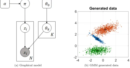
(a) Graphical model (b) GMM generated data
Figure 2.1: Probabilistic graphical model of the Bayesian mixture model. In the Gaussian caseθ = (µ,Σ) andθ0= (m0, c0, b0, a0).
2.3.2
Gibbs sampling
Where the E-M algorithm is the usual choice for inference in the GMM from Section2.2, inference in complex Bayesian models is usually performed usingMarkov chain Monte Carlo (MCMC) methods. Recall that the E-M algorithm is a maximum likelihood approach and so only guaranteed to find locally optimal fit of the model to the data. By contrast, the Gibbs sampler, introduced in (Geman & Geman,1984), is a randomized algorithm and as with all MCMC methods is asymptotically (that is, after an infinite number of iterations) guaranteed to find the global posterior distribution of the model. Unfortunately these asymptotic guarantees are not very useful in practice, as we never have unconstrained computational resources at our disposal and the Gibbs sampler can take a prohibitively large number of iterations to converge to the posterior distribution. This is worsened bypoor mixingof the sampler when the required posterior consists of few “islands” of states with high probability surrounded by an “ocean” of small non-zero probability. Gibbs sampling can also be seen as a specific case of the Metropolis-Hasting (M-H) algorithm, which in its varying forms can better handle discontinuities in the posterior state space. This thesis does not explore M-H in detail, but we would direct the reader to (Chib & Greenberg,1995) for an intuitive presentation.
Each step of the Gibbs sampler involves replacing the value of one of the variables in the model by a value drawn from the distribution of that variable conditioned on the values of the rest of the vari-ables in the model. For the Bayesian GMM (2.9), the varivari-ables (parameters and latent varivari-ables) would be {z1, ...zN, µ1, ..., µK,Σ1, ...,ΣK, π1, ..., πK}. Gibbs iterations would involve sampling the mixture
com-ponent parametersµ1, ..., µK and Σ1, ...,ΣK; the mixture coefficients π1, ..., πK and the cluster indicators
z1, ..., zK given the datax1, ..., xN. At each iteration, holding the rest of the quantities fixed, we will update
eachzi by drawing samples from the categorical distribution defined with weights for each categorykbeing:
p(zi=k|µk,Σk, πk, x) =
πkN(xi|µk,Σk)
PK
j=1πjN(xi|µj,Σj)
(2.13)
for k = 1, ..., K. Conditioned on the parameters {µ,Σ, π}, the probability of component assignments is computed in the same way as in (2.5). Once the indicator variables have been updated, we proceed by drawing samples now for the component parameters holding the rest of the quantities fixed:
(µk,Σk)∼NIW (µ,Σ|mk, ck, ak, bk) (2.14)
The parameters (mk, ck, bk, ak) of this NIW distribution depend upon the current values of the indicators
and are updated using:
mk =c0mc00++NNkx¯k k ck =c0+Nk ak =a0+Nk bk =b0+S+cc0Nk 0+Nk(¯xk−m0) (¯xk−m0) T (2.15) where ¯xk= P i:zi=kxi
Nk ;Nkdenotes the number of observations assigned to clusterkandS=
PK
i=1(xi−x¯k) (xi−x¯k) T
is the sample covariance matrix. Note that while (m0, c0, b0, a0) denote the prior terms of the NIW
distri-bution and should be specified a priori, (mk, ck, bk, ak) are the corresponding posterior terms of the NIW
posterior estimated using the data and the information about the prior. We emphasize the fact that the values of the parameters (mk, ck, bk, ak) are different for each cluster.
The next step is to sample the mixing coefficients from the following (posterior) Dirichlet distribution:
The posterior over the mixture weights is a Dirichlet distribution and so keeps the form of its conjugate prior, as expected. The algorithm iterates between sampling each of the random quantities until convergence, however note that convergence in MCMC methods has a different meaning. In the case of E-M for GMM, the complete data likelihood (or equivalently the negative log likelihood (NLL)−ln (p(x, z|µ,Σ, π)) in (2.17)) eventually stops increasing (choosing a small threshold value for these changes in likelihood suffices to stop the algorithm when the solution is sufficiently accurate). In Gibbs sampling though the likelihood never converges onto single point solution as it is stochastic. Instead, Gibbs sampling converges onto the required (by design) stationary posterior distribution. Detecting this type of convergence is a complex, well studied and yet still unresolved problem. There are a plethora of possible convergence diagnostics, but none of them provide any theoretical guarantees. Most of them rely on computing at each iteration the complete data likelihood: p(x, z|µ,Σ, π) = N Y i=1 K Y k=1 πδzi,k k p(xi|µk,Σk) δzi,k (2.17)
whereδzi,k is the Kronecker delta. Then, at convergence the sequence of values of p(x, z|µ,Σ, π) estimated
for consecutive iterations of the sampler should be independent; there should be no correlation between successive draws of the Gibbs sampler. In practice this can be quite hard to assess as it involves executing many iterations of the sampler ahead to check for correlations. In this thesis we rely on one of the most widely-used convergence diagnostics for Gibbs sampling described in (Raftery & Lewis, 1992). We provide a short outline of Gibbs sampling for the special case of inference in the spherical Bayesian GMM and this can be found in Chapter3, Algorithm3.3.
In the more general exponential family formulation of the mixture model (2.10), the Gibbs sampler iterates between updates for the indicatorsz1, . . . , zN, the parametersθ1, . . . , θK and the mixing parameters
π1, . . . , πK. Eachzi is updated by sampling from the categorical distribution with weights:
p(zi=k|θk, πk, x) =
πkexp (hg(xi), θki −ψ(θk)−h(xi))
PK
j πjexp (hg(xi), θji −ψ(θj)−h(xi))
(2.18)
for each componentk= 1, . . . , K. The component parameters for eachkare sampled from the posterior:
θk ∼G0(τk, ηk) (2.19)
withτk=τ+Pj:zj=kg(xj) andηk=η+Nk. The mixture coefficientsπin the more general setup are still
updated from the corresponding Dirichlet posterior from (2.16).
2.3.3
Variational Bayes inference
Variational methods provide a ubiquitous and general framework to convert the problem of stochastic infer-ence to one of deterministic optimization. They have played a key role across many application domains, however here we will briefly review them in the context of probabilistic modeling with the example of the GMM. When doing inference in probabilistic models, we are most often interested in the posterior over all the unknown variables p(Z|x). More precisely, often we try to evaluate the expectation of the complete data log-likelihood (the model log-likelihood) with respect to this posterior. However, this marginalization is rarely tractable, especially in Bayesian models where we have placed a prior distribution over the unknown quantities in the model (the parameters). We already presented one way to approximate stochastically this
expectation using MCMC methods (Gibbs sampler Section2.3.2); VB methods are deterministic. Consider the distributionq(Z) which approximates the posteriorp(Z|x), the log marginal probability of the data can then be written as:
lnp(x) =L(q) + KL (qkp) (2.20) where we use: L(q) = Z q(Z) ln p(x, Z) q(Z) dZ KL (qkp) = − Z q(Z) ln p(Z|x) q(Z) dZ (2.21)
The quantityL(q) can be seen as the lower bound of the posteriorp(Z|x), while KL (qkp) is the Kullback-Liebler divergence between the approximateq(Z) and the true posterior p(Z|x). In VB inference we aim to maximize the lower bound L(q), or equivalently minimize KL (qkp), which implies optimization with respect toq(Z). If no restrictions are placed on the type of distributionsq(Z), the maximum of the lower bound is obtained when the KL divergence vanishes sinceq(Z)≡p(Z|x). As this scenario is not tractable, typically restrictions are placed