Computational analysis of non-Newtonian boundary layer flow of Nanofluid past a vertical plate with partial slip

Computational analysis of non­Newtonian 

boundary layer flow of Nanofluid past a 

vertical plate with partial slip

Beg, OA, Rao, AS, Nagendra, N, Amanulla, CH and Reddy, MSN

Title

Computational analysis of non­Newtonian boundary layer flow of 

Nanofluid past a vertical plate with partial slip

Authors

Beg, OA, Rao, AS, Nagendra, N, Amanulla, CH and Reddy, MSN

Type

Article

URL

This version is available at: http://usir.salford.ac.uk/42310/

Published Date

2017

USIR is a digital collection of the research output of the University of Salford. Where copyright 

permits, full text material held in the repository is made freely available online and can be read, 

downloaded and copied for non­commercial private study or research purposes. Please check the 

manuscript for any further copyright restrictions.

For more information, including our policy and submission procedure, please

contact the Repository Team at: [email protected].

MODELLING, MEASUREMENT AND CONTROL B

Publisher: Association pour la promotion des techniques de modelisation et de simulation dans l'entreprise Press

ISSN 12595969

Accepted May 8

th

2017

COMPUTATIONAL ANALYSIS OF NON-NEWTONIAN BOUNDARY LAYER FLOW OF

NANOFLUID PAST A VERTICAL PLATE WITH PARTIAL SLIP

A Subba Rao1*, N Nagendra1, CH Amanulla1, 2, M Surya Narayana Reddy2 and O. Anwar Bég3 1_{Department of Mathematics, Madanapalle Institute of Technology and Science, Madanapalle-517325, India.}

2_{Department of Mathematics, JNTU College of Engineering, Pulivendula-516390, Andrapradesh, India.}

3_{Fluid Mechanics, Nanosystems and Propulsion, Aeronautical and Mechanical Engineering, School of Computing, Science and} Engineering, Newton Building, University of Salford, Manchester M54WT, United Kingdom.

Email: [email protected]

ABSTRACT

In the present study, the heat, momentum and mass (species) transfer in external boundary layer flow of Casson nanofluid over a vertical plate surface with multiple slip effect is studied theoretically. The effects of Brownian motion and thermophoresis are incorporated in the model in the presence of both heat and nanoparticle mass transfer convective conditions. The governing partial differential equations (PDEs) are transformed into highly nonlinear, coupled, multi-degree non-similar partial differential equations consisting of the momentum, energy and concentration equations via appropriate non-similarity transformations. These transformed conservation equations are solved subject to appropriate boundary conditions with a second order accurate finite difference method of the implicit type. The influences of the emerging parameters i.e. Casson fluid parameter (β), Brownian motion parameter (Nb), thermophoresis parameter (Nt), Buoyancy ratio parameter (N ), Lewis number (Le), Prandtl number (Pr), Velocity slip factor (Sf) and Thermal slip factor (ST) on velocity, temperature and nano-particle concentration distributions is illustrated graphically and interpreted at length. Validation of solutions with a Nakamura tridiagonal method has been included. The study is relevant to enrobing processes for electric-conductive nano-materials, of potential use in aerospace and other industries.

Keywords: Nanoparticles, Species diffusion, Casson viscoplastic model, Partial slip, Keller-box numerical method.

1.INTRODUCTION

The word “nanotechnology” was probably used for the first time by the Japanese scientist Norio Taniguchi in 1974. K. Eric Drexler is credited with initial theoretical work in the field of nanotechnology. The term nanotechnology was used by Drexler in his 1986 book “Engines of creation: The coming era of nanotechnology”. Drexler’s idea of nanotechnology is referred to as molecular nanotechnology [1]. Earlier the great theoretical physicist Richard Feynman predicted nanotechnology in 1959. In the 1980s and 1990s new nano-materials were discovered and nanofluids emerged as a result of the experiments intended to increase the thermal conductivity of liquids. The birth of nanofluids is attributed to the revolutionary idea of adding solid particles into fluids to increase the thermal conductivity. This innovative idea was put forth by the Scottish physicist J.C. Maxwell as early as 1873. Nanofluids have evolved into a very exciting and rich frontier in modern nano-technology. The excitement can be attributed to the robustness of the concept of nanofluids and the plethora of different applications of this technology [2] .The properties of nanofluids need a lot of fine tuning, many seemingly contradicting studies need clarity and validation. Nanofluids have potential applications in micro-electronics, fuel cells, rocket propulsion, environmental de-toxification, spray coating of aircraft wings, pharmaceutical suspensions, medical sprays etc. These applications of nanofluids are largely attributable to the enhanced thermal conductivity and Brownian motion dynamics which can be exploited to immense benefit. Nanomaterials work efficiently as new energy materials since they incorporate suspended particles with size as the same as or smaller than the size of de Broglie wave [3]. The use of nanoparticles is now a subject of abundant studies, and aspects of particular interest are Brownian motion and thermophoretic transport. Nanofluids constitute a new class of heat transfer fluids comprising a conventional base fluid and nano-particles. The nanoparticles are utilized to enhance the heat transfer performance of the base fluids [4]. The cooling rate requirements cannot be obtained by the ordinary heat transfer fluids because their thermal conductivity is not adequate. Brownian motion of the nanoparticles enhances the thermal conductivity of base fluids, although there may be many more mechanisms at work which exert a contribution. The concept of nanofluids was introduced by Choi [5] wherein he proposed the suspension of nanoparticles in a base fluid such as water, oil, and ethylene glycol. Buongiorno [6] attempted to explain the increase in the thermal conductivity of such fluids and developed a model that emphasized the key mechanisms in laminar flow as being particle Brownian motion and thermophoresis.

In recent years with the development of hydrophobic surfaces, slip flows have garnered some attention in nanofluid dynamics. Furthermore the non-Newtonian properties of different nanofluid suspensions have also attracted interest in simulating rheological behavior with different models. Noghrehabadi et al. [7] investigated the effects of the slip boundary condition on the heat transfer characteristics for a stretching sheet subjected to convective heat transfer in the presence of nanoparticles. They found that the flow velocity and the surface shear stress on the stretching sheet are strongly influenced by the slip parameter with a decrease in the momentum boundary layer thickness and increase in thermal boundary layer thickness. Khan and Pop [8] studied the problem of laminar fluid flow which results from a stretching of a flat surface in a nanofluid. They analyzed the development of the steady boundary layer flow, heat transfer and nanoparticle volume fraction, observing that the reduced Nusselt number decreased while the reduced Sherwood number increased with greater volume fraction. Subba Rao and Nagendra [9] investigated thermal radiation effects on Oldroyd-B viscoelastic nanofluid flow from a stretching sheet in a non-Darcy porous medium. They analyzed the behavior of nano particles on temperature and concentration distributions in detail. Uddin et al. [10] analyzed anisotropic slip effects on nanofluid bioconvection boundary layers from a translating sheet using MAPLE symbolic quadrature and Lie group methods. Rana et al. [11] used a high-penalty finite element method to simulate two-dimensional flow dissipative viscoelastic nanofluid polymeric boundary layer stretching sheet flow, employing the Reiner-Rivlin second grade non-Newtonian model. They showed that greater polymer fluid viscoelasticity accelerates the flow and increasing Brownian motion and thermophoresis enhances temperatures and reduces heat transfer rates (local Nusselt numbers. Malik et al. [12] used the Runge–Kutta Fehlberg method to obtain numerical solutions for steady thermal boundary layer flow of a Casson nanofluid flowing over a vertical radially exponentially-stretching cylinder. Many such studies have been communicated and have usually adopted the so-called “active control” boundary condition, based on the Kuznetsov-Nield formulation [13] for natural convective boundary layer flow of a nanofluid over a vertical surface featuring Brownian motion and thermophoresis. However Kuznetsov and Nield [14] re-visited their original model, refining this formulation with passive control of nanofluid particle fraction at the boundary rather than active control to be more physically realistic. This recent boundary condition provides one of the motivations for the present research. Uddin and Bég [15] obtained extensive solutions for the influence of multiple slip and radiative heat transfer on magnetized stretching sheet flow for a range of thermal and mass convective boundary conditions. Further studies of magnetic non-Newtonian and/or slip transport of nanofluids include Ahmed and Mahdy [16] (for bioconvection nanofluids over wavy surfaces), the above studies were generally confined to internal transport. However external boundary layer convection flows also find applications in many technological systems including enrobing polymer coating processes, heat exchanger design, solar collector architecture etc. Prasad et al. [17] studied two-dimensional nanofluid boundary layer flow from a spherical geometry embedded in porous media with a finite difference scheme. Sarojamma and Vendabai [18] investigated computationally the heat and mass transfer in magnetized Casson nanofluid boundary layer flow from a vertical exponentially stretching cylinder with heat source/sink effects.

The present work, motivated by applications in enrobing dynamics of nanomaterials, examines theoretically and computationally the steady-state transport phenomena in Casson nanofluid flow over a vertical plate with partial slip. Mathematical modelling is developed to derive the equations of continuity, momentum, energy and species conservation, based on the Buonjiornio nanofluid model [6]. The partial differential boundary layer equations are then transformed into a system of dimensionless non-linear coupled differential boundary layer equations, which is solved with the robust second order accurate Keller box implicit finite difference method. The present work extends significantly earlier simulations of Hussain et al. [19] (who consider an exponentially stretching surface) to the case of a vertical plate with partial slip condition. An extensive parametric analysis of the influence of a number of parameters (Brownian motion, thermophoresis, Casson non-Newtonian, Biot number, stream wise coordinate) on thermo-diffusive characteristics is conducted. The simulations are also relevant to calendering in pseudo-plastic materials fabrication [20].

2.MATHEMATICAL MODEL

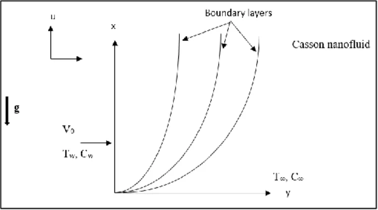
We examine steady buoyancy-driven convection heat transfer flow of Casson nanofluid from a vertical plate. Figure 1 shows the flow model and associated coordinate system.

The nanofluid fluid is taken to be incompressible and a homogenous dilute solution. The x-coordinate is measured along the vertical plate from the lowest point and the y-coordinate is measured normal to the surface. The gravitational acceleration, g acts downwards. Both the plate and the fluid are maintained initially at the same temperature. Instantaneously they are raised to a temperature

T

_w



T

_ i.e. the ambient temperature of the fluid which remains unchanged. The appropriate constitutive equations for the Casson non-Newtonian model are:

2 , 2 2 , 2 y B ij c ij y B ij c c p e p e                _ _       _{ }             (1)

in which





e e

_{ij ij} and

e

_ij is the (i,j)th _{component of deformation rate, π denotes the product of the component of} deformation rate with itself, πc shows a critical value of this product based on the non-Newtonian model,



_B the plastic dynamic viscosity of non-Newtonian fluid and p_y the yield stress of fluid. The Casson model, although relatively simple, is a robust viscoplastic model and describes accurately the shear stress-strain behavior of certain industrial polymers in which flow is not possible prior to the attainment of a critical shear stress. Unlike the Bingham viscoplastic model which has a linear shear rate, the Casson model has a non-linear shear rate. Casson fluid theory was originally propounded to simulate shear thinning (viscosity is reduced with greater shear rates) liquids containing rod-like solids and is equally popular in analysing inks, emulsions, food stuffs (chocolate melts), certain gels and paints [21]. More recently it has been embraced in advanced polymeric flow processing [22]. Incorporating the Casson terms and applying the Buonjiorni nanofluid model, the governing conservation equations, in primitive form, for the regime under investigation i.e. mass continuity, momentum, energy and species, can be written as follows:

0 u v x y  _ _   (2) 2 2 1 1 T( ) C( ) u u u u v g T T g C C x y   y        _  _{ }  _{   }       (3) 2 2 2 T B D T T T C T T u v D x y  y  y y T y  _{ }   _  _  _{ }   _  _        _   _ _{ } (4) 2 2 2 2 T B D C C C T u v D x y y T y  _  _  _      (5) The boundary conditions imposed at the vertical plate surface and in the free stream are:

0 0 Aty 0,u N u,v 0,T T_w K T y y          Asy  ,u 0,v0,TT,CC (6)

HereN0 is the velocity slip factorK0is the thermal slip factor and T is the free stream temperature. ForN0  0 K0, one can recover the no-slip case. The u and v are the velocity components in the x- and y- directions respectively, ν- the kinematic viscosity of the electrically-conducting nanofluid, β - is the non-Newtonian Casson parameter respectively, f is the density of

fluid,  is the electrical conductivity of the nanofluid, _{- the thermal diffusivity of the nanofluid,} T - the temperature, respectively. Furthermore  

   

c _p/ c _f is the ratio of nanoparticle heat capacity and the base fluid heat capacity, C_p is the specific heat capacity; DB is the Brownian diffusion coefficient;DT is the thermophoretic diffusion coefficient; k is the thermal

conductivity of nanofluid; T_wand C_are the ambient fluid temperature and concentration, respectively.

The stream function  is defined by the Cauchy-Riemann equations, u  y andv  x, and therefore,

the continuity equation is automatically satisfied. In order to write the governing equations and the boundary conditions in dimensionless form, the following non-dimensional quantities are introduced.

 

1/4

 

1/4 0 _{, , 4 ( , )} 1 4 x x V x y Gr Gr f x              _  _  





3 2 ( , ) , ( , ) , 4 T w x w w g T T x T T C C Gr T T C C                      (7)

The transformed boundary layer equations for momentum, energy and concentration emerge as:





2 1 1 f 3f f 2f N f f f f          _{  }             _ _   _  _     (8)





2 3 Pr b t f f N N f  _{     }  _    _{   }  _ _       _  _     (9)





1 3 b t N f f f Le Le N  _{   }  _   _{   }  _ _{ }   _{ }    (10)

The corresponding transformed dimensionless boundary conditions are: 1 At 0, 0, 1 (0), 1 (0) β f T f f S f S   _  _        As  ,f 0, 0, 0       (11) where Pr = / is Prandtl number; Gr is a Grashof buoyancy number; 1/ 4

0 /

f

S N Gr xandST K Gr₀ 1/4/xthe non-dimensional velocity slip and thermal jump parameters. Le/DB is the Lewis number; Nt

 

c pDT



TwT

  

/ c f T is the

thermophoresis parameter;Nb

 

c _pD_B



C_wC_

  

/ c _f is the Brownian parameter; Nβ (C CwC) / β (T TwT) is the

concentration to thermal buoyancy ratio parameter. All other parameters are defined in the nomenclature. The skin-friction coefficient (plate surface shear stress function), the local Nusselt number (heat transfer rate) and Sherwood number (mass transfer rate) can be defined using the transformations described above with the following expressions:

3 4 1 1 1 ( , 0) 4Grx Cf  f   _{ }  _  _   (12) 1 4 _{( , 0)} x Gr Nu   (13) 1 4 _{( , 0)} x Gr Sh   (14)

3. NUMERICAL SOLUTION WITH KELLER BOX IMPLICT METHOD

The strongly coupled, nonlinear conservation equations do not admit analytical (closed-form) solutions. An elegant, implicit difference finite difference numerical method developed by Keller [23] is therefore adopted to solve the general flow model defined by equations (8)-(10) with boundary conditions (11). This method is especially appropriate for boundary layer flow equations which are parabolic in nature. It remains one of the most widely applied computational methods in viscous fluid dynamics. Recent problems which have used Keller’s method include natural convection flow of a chemically-reacting Newtonian fluid along vertical and inclined plates [24], stretching sheet MHD flow of Casson fluid model [25], magnetohydrodynamic Falkner-Skan “wedge” flows [26], magneto-rheological flow from an extending cylinder [27], Hall magneto-gas dynamic generator slip flows [28] and radiative-convective Casson slip boundary layer flows [29]. Keller’s method provides unconditional stability and rapid convergence for strongly non-linear flows. It involves four key stages, summarized below.

1) Reduction of the Nth order partial differential equation system to N first order equations 2) Finite difference discretization of reduced equations

3) Quasilinearization of non-linear Keller algebraic equations

4) Block-tridiagonal elimination of linearized Keller algebraic equations

Stage 1: Reduction of the Nthorder partial differential equation system to N first order equations

Equations (8) – (10) and (11) subject to the boundary conditions are first written as a system of first-order equations. For this purpose, we reset Equations (6) – (7) as a set of simultaneous equations by introducing the new variables.

f u (15)

'

s





₍₁₇₎ s t (18) g  p (19)





2 1 1 v 3f  v 2u (s Ng)  u u v f      _                _{ }      (20)



₃



2 Pr b t t s f f  t N t N t  u t    _          _  _     (21)





1 3 b t N p g f f p t u p Le  Le N     _         _  _     (22) where primes denote differentiation with respect to



.

In terms of the dependent variables, the boundary conditions become:

At 0 : 0, 0, 1, 1 As : 0, 0, 0, 0 u f s g u v s g              (23)

Stage 2: Finite difference discretization of reduced boundary layer equations

A two-dimensional computational grid (mesh) is imposed on the -η plane as sketched in Fig.2. The stepping process is defined by: 0 0, j j1 h j_j, 1, 2,..., ,J _J





 

   







_ (24) 0 _0, n n1 _{, 1, 2,...,} n k n N



_



_



 _{ } (25)

where kn and hj denote the step distances in the ξ (streamwise) and η (spanwise) directions respectively.

Figure. 2 Keller Box element and boundary layer mesh If n

j

g denotes the value of any variable at



 j, n



, then the variables and derivatives of Eqns. (15) – (22) at





1/ 2 1/ 2, n j     are replaced by:





1/ 2 1 1 1/ 2 1 1 1 4 n n n n n j j j j j g  g g g  g (26)





1/ 2 1 1 1 1 1/ 2 1 2 n n n n n j j j j j j g g g g g h          _{   } _    (27)





1/ 2 1 1 1 1 1/ 2 1 2 n n n n n j j j j n j g g g g g k          _{   } _    (28)





1 1 1/ 2 n n n j j j j h f f _ u _ (29)





1 1 1/ 2 n n n j j j j h u u  v (30)





1 1 1/ 2 n n n j j j j h g g _ p _ (31)





1 1 1/ 2 n n n j j j j h    t  (32)







































 

1 1 1 1 1 1 2 1 1/ 2 1 1 1 1 1/ 2 1 1 1/ 2 3 1 1 4 ( ) 2 2 2 2 4 2 j j j j j j j j j j j j j j j j n j j j j j j n j n j j j j h v v f f v v h h v v s s N g g h h f v v u u h v f f R                     _   _  _{     }   _{ }                 (33)



















































 

1 1 1 2 1 1 1 1 1 1 1/2 1 1 1 1/2 1 1/2 1 1 1/2 1 1 2 _1/2 3 1 Pr 4 4 4 4 2 2 2 2 2 j j j j j j j j j j j j j j j j j n j j j j j j j j n j n j j j j j j j n j j j j j j _j h t t f f t t h h Nt t t u u s s h h Nb t t p p s u u h h u s s f t t h h t f f t t R                             _  _{ }   _   _      _   _    _   _           n1 (34)































 











1 1 1 1 1 1 1/2 1 1 1 1/2 1 1 1 1 1 1/2 1 1/2 1 3 _1/2 3 1 4 4 2 2 2 2 j j j j j j j j j n j j j j j j j j n j j j j j j j n j n j n j j j j j j _j h p p f f p p Le h h u u g g s u u h B t t u g g p p Le h h f p p p f f R                            _  _{ }   _   _    _   _              _{ } (35)

Where the following notation applies:

1/2 , n n Nt B k Nb     (36)

 



















2 1 1/ 2 1 1 _{1/ 2} 1/ 2 1/ 2 1/ 2 1/ 2 1 1 2 3 j j j j n j j j j j j v v u h R h f v s Ng             _{ } _   _  _      _{ }             _{ }        (37)

 



 





   

1 1/2 1/2 1/2 1/2 1 2 _1/2 2 1/2 1/2 1/2 1 Pr 3 j j j j j j n j j j j j j t t u s Nb p t h R h f t Nt t                _               _   _ _{   }      (38)











1 1/2 1/2 1 3 _1/2 1 1/2 1/2 1 3 j j j j j n j j j j j j j p p f p Le h R h t t B u g Le h                           _{ }          _{ }           _{ }    (39)

The boundary conditions are

0 0 0, 0 1, 0, 0, 0, 0 1, 0

n n n n n n n n

J J J J

f u 



 u  v 











 (40)

Stage 3: Quasilinearization of non-linear Keller algebraic equations

If we assume 1 1 1 1 1 1 1, 1, 1, 1, 1, 1,

n n n n n n

j j j j j j

f  u v p  s t  to be known for , Equations (29) – (35) comprise a system of

6J+6 equations for the solution of 6J+6 unknownsf_jn,un_j,vn_j, pn_j,sn_j,tn_j, j = 0, 1, 2 …, J. This non-linear system of algebraic

equations is linearized by means of Newton’s method as elaborated by Keller [23] and explained in [36,37].

Stage 4: Block-tridiagonal elimination of linear Keller algebraic equations

The linearized version of eqns. (29) – (35) can now be solved by the block-elimination method, since they possess a

block-tridiagonal structure since it consists of block matrices. The complete linearized system is formulated as a block matrix

system, where each element in the coefficient matrix is a matrix itself. Then, this system is solved using the efficient Keller-box

method. The numerical results are affected by the number of mesh points in both directions. After some trials in the η-direction (radial coordinate) a larger number of mesh points are selected whereas in the ξ direction (tangential coordinate) significantly less mesh points are utilized. ηmax has been set at 16 and this defines an adequately large value at which the prescribed boundary conditions are satisfied. ξmax is set at 1.0 for this flow domain. Mesh independence testing is also performed to ensure that the converged solutions are correct. The computer program of the algorithm is executed in MATLAB running on a PC.

If we assume fjn,unj,vnj, pnj,snj,tnj,to be known for

0

 

j

J

, Eqs. (29) - (35) are a system of 6J+6 equations for the

solution of 6J+6 unknowns fjn,unj,vnj, pnj,snj,tnj,, j = 0, 1, 2 … J. This non-linear system of algebraic equations is linearized by

means of Newton’s method which then solved in a very efficient manner by using the Keller-box method, which has been used most efficiently by Cebeci and Bradshaw[38], taking the initial interaction with a given set of converged solutions at   n_{. To}

initiate the process with



0, we first prescribe a set of guess profiles for the functions f u v, , , and t which are

unconditionally convergent. These profiles are then employed in the Keller-box scheme with second-order accuracy to compute

the correct solution step by step along the boundary layer. For a given



the iterative procedure is stopped to give the final velocity and temperature distribution when the difference in computing these functions in the next procedure become less than

5

10 , i.e., 5

10 ,

i f



_  _{where the superscript idenotes the number of iterations.}

For laminar flows the rate of convergence of the solutions of the equations (29)-(35) is quadratic provided the initial estimate to the desired solution is reasonably close to the final solution. Calculations are performed with four different  spacings show that the rate of convergence of the solutions is quadratic in all cases for these initial profiles with typical iterations. The fact that Newton’s method is used to to linearize the non-linear algebraic equations and that with proper initial guess_nusually obtained from a solution at _n1, the rate of convergence of the solutions should be quadratic can be used to test the code for possible programming errors and to aid in the choice of  spacings in the downstream direction. To study the effect of  spacing on the rate of convergence of solutions, calculations were performed in the range 0  0.4 with uniform 



spacings corresponding to 0.08, 0.04, 0.02 and 0.01. Except for the results obtained with  =0.08, the rate of convergence of the solutions was essentially quadratic at each



station. In most laminar boundary layer flows, a step size of  y 0.02to 0.04 is sufficient to provide accurate and comparable results. In fact in the present problem, we can even go up to  y 0.1and still get accurate and comparable results. This particular value of  y 0.1 has also been used successfully by Merkin [39]. A uniform grid across the boundary is quite satisfactory for most laminar flow calculations, especially in laminar boundary layer. However, the Keller-box method is unique in which various spacing in both  and  directions can be used (Aldoss et al.,[40]).

4. VALIDATION WITH NAKAMURA DIFFERENCE SCHEME

The present Keller box method (KBM) algorithm has been tested rigorously and benchmarked in numerous studies by the authors. However to further increase confidence in the present solutions, we have validated the general model with an

alternative finite difference procedure due to Nakamura [30]. The Nakamura tridiagonal method (NTM) generally achieves fast convergence for nonlinear viscous flows which may be described by either parabolic (boundary layer) or elliptic (Navier-Stokes) equations. The coupled 7th order system of nonlinear, multi-degree, ordinary differential equations defined by (8)–(10) with boundary conditions (11) is solved using the NANONAK code in double precision arithmetic in Fortran 90, as elaborated by Bég [31]. Computations are performed on an SGI Octane Desk workstation with dual processors and take seconds for compilation. As with other difference schemes, a reduction in the higher order differential equations, is also fundamental to Nakamura’s method. The method has been employed successfully to simulate many sophisticated nonlinear transport phenomena problems e.g. magnetized bio-polymer enrobing coating flows (Bég et al. [32]). Intrinsic to this method is the discretization of the flow regime using an equi-spaced finite difference mesh in the transformed coordinate () and the central difference scheme is applied on the -variable. A backward difference scheme is applied on the -variable. Two iteration loops are used and once the solution for  has converged, the code progresses to the next  station. The partial derivatives for f,,  with respect to  are as explained evaluated by central difference approximations. An iteration loop based on the method of successive substitution is utilized to advance the solution i.e. march along. The finite difference discretized equations are solved in a step-by-step fashion on the 

-domain in the inner loop and thereafter on the -domain in the outer loop. For the energy and nano-particle species conservation Eqns. (9)-(10) which are second order multi-degree ordinary differential equations, only a direct substitution is needed. However a reduction is required for the third order momentum (velocity) boundary layer eqn. (8). We apply the following substitutions:

P f (41)

Q (42)

R (43)

The eqns. (8)-(10) then retract to:

Nakamura momentum equation:

(44)

Nakamura energy equation:

(45)

Nakamura nano-particle species equation:

(46)

Here Ai=1,2,3, Bi=1,2,3, Ci=1,2,3, are the Nakamura matrix coefficients, Ti=1,2,3, are the Nakamura source terms containing a mixture of variables and derivatives associated with the respective lead variable (P, Q, R). The Nakamura Eqns. (27)–(30) are transformed to finite difference equations and these are orchestrated to form a tridiagonal system which due to the high nonlinearity of the numerous coupled, multi-degree terms in the momentum, energy, nano-particle species and motile micro-organism density conservation equations, is solved iteratively. Householder’s technique is ideal for this iteration. The boundary conditions (11) are also easily transformed. Further details of the NTM approach are provided in Nakamura [30]. Comparisons are documented in Table. 1 for skin friction and very good correlation is attained. Table. 1 further indicates that increase in Casson viscoplastic parameter (β) induces a strong retardation in the flow i.e. suppresses skin friction magnitudes. In both cases however positive magnitudes indicate flow reversal is not generated.

5. KELLER BOX METHOD (KBM) NUMERICAL RESULTS AND DISCUSSION

Comprehensive solutions have been obtained with KBM and are presented in Figures 3 to 11. The numerical problem comprises three dependent thermo-fluid dynamic variables



f, , 



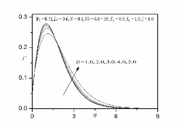
and eight multi-physical control parameters, Pr, Le, β, N, Nb,

Nt,Sf, ST. The influence of stream wise space variable  is also investigated.In the present computations, the following default parameters are prescribed (unless otherwise stated): Pr=0.71, Le=0.6, =1.0, N=0.1, Nb=0.4=Nt, Sf=0.5, ST=1.0, =1.0.

1 1 / 1 // 1

P

B

P

C

P

T

A







2 2 / 2 // 2Q B Q C Q T A    3 3 / 3 // 3R B R C R T A   

Figure. 3(a) Effect of β on velocity profiles

Figure. 3(b) Effect of β on temperature profiles

Figures. 3(a) – 3(c) illustrate the effect of the Casson viscoplastic parameter, on velocity

 

f , temperature

 

 and concentration

 

 profiles. With increasing, β values, initially close to the plate surface, fig. 3a shows that the flow is strongly decelerated. However, further from the surface, the converse response is induced in the flow. This may be related to the necessity for a yield stress to



_

_{1 1/  }

_

_{f (0)}

_

_{1 1/  }

_

_{f (0)} 0.7 0.8412 0.8411 1.2 0.7605 0.7607 1.6 0.7277 0.7261 2.0 0.7065 0.7061 3.0 0.9070 0.9073

Table 1. Numerical values of skin-friction coefficient



1 1/  



f (0)with various β.

be attained prior to viscous flow initiation in viscoplastic shear-thinning nanofluids. Within a short distance of the plate surface, however a strong acceleration is generated with greater Casson parameter. This serves to decrease momentum boundary layer thickness effectively. A similar observation has been reported by for example, Mustafa and Khan [33] and Makanda et al. [34]. The viscoplastic parameter modifies the shear term f /// in the momentum boundary layer equation (8) with an inverse factor, 1/β, and effectively assists momentum diffusion for β >1. This leads to a thinning in the hydrodynamic boundary layer and associated deceleration. The case β = 0 which corresponds to a Newtonian fluid is not considered. An increase in viscoplastic parameter however decreases both temperature and nano-particle concentration magnitudes throughout the boundary layer, although the

reduction is relatively weak. Thermal and nanoparticle concentration boundary layer thickness are both suppressed with greater viscoplasticity of the nanofluid.

Figure. 3(c) Effect of β on concentration profiles

Figure. 4(a) Effect of Pr on velocity profiles

Figure. 4(b) Effect of Pr on temperature profiles

Figures. 4(a)-4(c) depicts the effect of Prandtl number (Pr) on the velocity

 

f , temperature

 

 and nanoparticle concentration

 

 distributions with transverse coordinate (). Fig. 4a shows that with increasing Prandtl number there is a strong deceleration in the flow. The Prandtl number expresses the ratio of momentum diffusion rate to thermal diffusion rate.

Figure. 4(c) Effect of Pr on concentration profiles

When Pr is unity both momentum and heat diffuse at the same rate and the velocity and thermal boundary layer thicknesses are the same. With Pr > 1 there is a progressive decrease in thermal diffusivity relative to momentum diffusivity and this serves to retard the boundary layer flow. Momentum boundary layer thickness therefore grows with Prandtl number on the surface of the vertical plate. It is also noteworthy that the peak velocity which is achieved close to the plate surface is systematically displaced closer to the surface with greater Prandtl number. The asymptotically smooth profiles of velocity which decays to zero in the free stream, also confirm the imposition of an adequately large infinity boundary condition. Fig. 4b indicates that increasing Prandtl number also suppresses temperatures in the boundary layer and therefore reduces thermal boundary layer thickness. Prandtl number is inversely proportional to thermal conductivity of the viscoplastic nanofluid. Higher thermal conductivity implies lower Prandtl number and vice versa. With greater Prandtl number, thermal conductivity is reduces and this inhibits thermal conduction heat transfer which cools the boundary layer.The monotonic decays in fig. 4b are also characteristic of the temperature distribution in curved surface boundary layer flows. Inspection of fig. 4c reveals that increasing Prandtl number strongly elevates the nano-particle concentration magnitudes. In fact a concentration overshoot is induced near the plate surface. Therefore while thermal transport is reduced with greater Prandtl number, species diffusion is encouraged and nano-particle concentration boundary layer thickness grows.

Figures. 5(a) – 5(c) illustrate the evolution of velocity, temperature and concentration functions with a variation in the Lewis number, is depicted. Lewis number is the ratio of thermal diffusivity to mass (nano-particle) species diffusivity. Le =1 which physically implies that thermal diffusivity of the nanofluid and species diffusivity of the nano-particles are the same and both boundary layer thicknesses are equivalent. For Le < 1, mass diffusivity exceeds thermal diffusivity and vice versa for Le > 1. Both cases are examined in figs 5a-5c. In fig 5a, a consistently weak decrease in velocity accompanies an increase in Lewis number. Momentum boundary layer thickness is therefore increased with greater Lewis number. This is sustained throughout the boundary layer. Fig. 5b shows that increasing Lewis number also depresses the temperature magnitudes and therefore reduces thermal boundary layer thickness. Therefore judicious selection of nano-particles during doping of polymers has a pronounced influence on velocity (momentum) and thermal characteristics in enrobing flow, since mass diffusivity is dependent on the nat ure of nano-particle species in the base fluid. Fig 5c demonstrates that a more dramatic depression in nano-particle concentration results from an increase in Lewis number over the same range as figs. 5a,b. The concentration profile evolves from approximat ely linear decay to strongly parabolic decay with increment in Lewis number.

Figure. 5(b) Effect of Le on temperature profiles

Figures. 6(a) – 6(c) illustrate the variation of velocity, temperature and nano-particle concentration with transverse coordinate (), for different values of velocity slip factor (Sf). Velocity slip factor is imposed in the augmented wall boundary condition in eqn. (11). With increasing velocity slip factor, more heat is transmitted to the fluid and this energizes the boundary layer. This also leads to a general acceleration as observed in fig. 6a and also to a more pronounced restoration in temperatures in fig. 6b, in particular near the wall. Furthermore, the acceleration near the wall with increasing velocity slip effect has been computed by Subba Rao et al. [29] using Keller box method

.

The effect of velocity slip is progressively reduced with further distance from the wall (curved surface) into the boundary layer and vanishes some distance before the free stream. It is also apparent from fig. 6c that nanoparticle concentration is enhanced with greater Velocity slip effect. Momentum boundary layer thickness is therefore reduced whereas thermal and species boundary layer thickness are enlarged. Obviously the non-trivial responses computed in figs. 6a-c further emphasize the need to incorporate Velocity slip effects in realistic nanofluid enrobing flows.

Figure. 5(c) Effect of Le on concentration profiles

Figure. 6(b) Effect of Sf on temperature profiles

Figures. 7(a) – 7(c) illustrate the variation of velocity, temperature and nano-particle concentration with transverse coordinate (), for different values of thermal slip parameter (ST). Thermal slip is imposed in the augmented wall boundary condition in eqn. (11). With increasing thermal slip less heat is transmitted to the fluid and this de-energizes the boundary layer.

Figure. 6(c) Effect of Sf on concentration profiles

Figure. 7(b) Effect of ST on temperature profiles

This also leads to a general deceleration as observed in fig. 7a and also to a more pronounced depletion in temperatures in fig. 7b, in particular near the wall. The effect of thermal slip is progressively reduced with further distance from the wall (curved surface) into the boundary layer and vanishes some distance before the free stream. It is also apparent from fig. 7c that nanoparticle concentration is reduced with greater thermal slip effect. Momentum boundary layer thickness is therefore increased whereas thermal and species boundary layer thickness are depressed. Evidently the non-trivial responses computed in figs. 7a-c further emphasize the need to incorporate thermal slip effects in realistic nanofluid enrobing flows.

Figure. 7(c) Effect of ST on concentration profiles

Figure. 8(b) Effect of N on temperature profiles

Figures. 8(a) – 8(c) exhibit the profiles for velocity, temperature and concentration, respectively with increasing buoyancy ratio parameter, N.In general, increases in the value of N have the prevalent to cause more induced flow along the plate surface. This behavior in the flow velocity increases in the fluid temperature and volume fraction species as well as slight decreased in the thermal and species boundary layers thickness as N increases.

Figure. 8(c) Effect of N on concentration profiles

Figure. 9(b) Effect of Nt on temperature profiles

Figures. 9(a) – 9(c) illustrates the effect of the thermophoresis parameter (Nt) on the velocity

 

f , temperature   and concentration_{ } distributions, respectively. Thermophoretic migration of nano-particles results in exacerbated transfer of heat from the nanofluid regime to the plate surface. This de-energizes the boundary layer and inhibits simultaneously the diffusion of momentum, manifesting in a reduction in velocity i.e. retardation in the boundary layer flow and increasing momentum (hydrodynamic) boundary layer thickness, as computed in fig. 9a. Temperature is similarly decreased with greater thermophoresis parameter (fig. 9b). Conversely there is a substantial enhancement in nano-particle concentration (and species boundary layer thickness) with greater Nt values. Similar observations have been made by Kunetsov and Nield [14] and Ferdows et al. [35] for respectively, both non-conducting Newtonian and electrically-conducting Newtonian flows.

Figure. 9(c) Effect of Nt on concentration profiles

Figures. 10(a) – 10(c) depict the response in velocity_{ f} , temperature   and concentration  functions to a variation in the Brownian motion parameter (Nb). Increasing Brownian motion parameter physically correlates with smaller nanoparticle

diameters, as elaborated in Rana et al. [11]. Smaller values of Nb corresponding to larger nanoparticles, and imply that surface

area is reduced which in turn decreases thermal conduction heat transfer to the plate surface. This coupled with enhanced macro-convection within the nanofluid energizes the boundary layer and accelerates the flow as observed in fig. 10a. Similarly the energization of the boundary layer elevates thermal energy which increases temperature in the viscoplastic nanofluid. Fig 10c however indicates that the contrary response is computed in the nano-particle concentration field. With greater Brownian motion number species diffusion is suppressed. Effectively therefore momentum and nanoparticle concentration boundary layer thickness is decreased whereas thermal boundary layer thickness is increased with higher Brownian motion parameter values.

Figure. 10(b) Effect of Nb on temperature profiles

Figure. 10(c) Effect of Nb on concentration profiles

Figure. 11(a) Effect of  on velocity profiles

Figures. 11(a) – 11(c) present the distributions for velocity, temperature and concentration fields with stream wise coordinate , for the viscoplastic nanofluid flow. Increasing  values correspond to progression around the periphery of the

vertical palte, from the leading edge (=0). As  increases, there is a weak deceleration in the flow (fig. 11a), which is strongest nearer the plate surface and decays with distance into the free stream. Conversely there is a weak elevation in temperatures (fig. 11b) and nano-particle concentration magnitudes (fig. 11c) with increasing stream wise coordinate.

Figure. 11(b) Effect of  on temperature profiles

Figure. 11(c) Effect of  on concentration profiles

6. CONCLUSIONS

A theoretical study has been conducted to simulate the viscoplastic nanofluid boundary layer flow in enrobing processes from a vertical plate with Partial slip effect using the Buonjiornio formulation. The transformed momentum, heat and species boundary layer equations have been solved computationally with Keller’s finite difference method. Computations have been verified with Nakamura’s tridiagonal method. The present study has shown that:

(i) Increasing viscoplastic (Casson) parameter decelerates the flow and also decreases thermal and nano-particle concentration boundary layer thickness.

(ii) Increasing Prandtl number retards the flow and also decreases temperatures and nano-particle concentration values. (iii) Increasing stream wise coordinate decelerates the flow whereas it enhances temperatures and species (nano-particle)

concentrations.

(iv) Increasing velocity slip strongly enhances velocities and reduces temperatures and nano-particle concentrations. (v) Increasing thermal slip strongly reduces velocities, temperatures and nano-particle concentrations.

(vi) Increasing Brownian motion accelerates the flow and enhances temperatures whereas it reduces nanoparticle concentration boundary layer thickness.

(vii) Increasing thermophoretic parameter increases momentum (hydrodynamic) boundary layer thickness and nanoparticle boundary layer thickness whereas it reduces thermal boundary layer thickness.

The current study has explored an interesting viscoplastic model for nanomaterials which are currently of interest in aerospace coating applications. Time-dependent effects have been neglected. Future studies will therefore address transient enrobing viscoplastic nanofluid transport phenomena for alternative geometries (wedge, cone, sphere), also of interest in aerospace materials fabrication and will be communicated imminently.

ACKNOWLEDGEMENTS

The authors appreciate the constructive comments of the reviewers which led to definite improvement in the paper. The corresponding author Dr. A. Subba Rao is thankful to the management of Madanapalle Institute of Technology & Science, Madanapalle for providing research facilities.

REFERENCES

[1] Kleinstreuer, C. and Feng, Y., “Experimental and theoretical studies of nanofluid thermal conductivity enhancement: a review”, Nanoscale Research Letters., vol. 6, pp. 229. 2011.Doi:10.1186/1556-276X-6-229..

[2] Wong, K.V., and Deleon, O., “Applications of nanofluid-current and future”, Advances in Mechanical Engineering., vol. 1, pp. 11. 2010.

Doi:10.1155/2010/519659.

[3] Sharma, A., Tyagi, V.V., Chen, C.R. and Buddhi, D., “Review on thermal energy storage with phase change materials and applications”, Renewable and Sustainable Energy Reviews., vol. 13, pp. 318 -345. 2009.

Doi:10.1016/j.rser.2007.10.005.

[4] Choi, S.U.S., and Eastman, J.A., “Enhancing thermal conductivity of fluids with nanoparticles”, ASME International

Mechanical Engineering Congress & Exposition, San Francisco, USA, vol. 66, pp. 99-105. 1995.

[5] Choi, S., “Enhancing thermal conductivity of fluids with nanoparticles”, ASME-Publ. Fluids Engineering Division., vol. 231, pp. 99–106.1995.

[6] Buongiorno, J., “Convective transport in nanofluids”, ASME J. Heat Trans., vol. 128, pp. 240–250. 2006.

Doi:10.1115/1.2150834.

[7] Noghrehabadi, A., Pourrajab, R., Ghalambaz, M., “Effect of partial slip boundary condition on the flow and heat transfer of nanofluids past stretching sheet prescribed constant wall temperature:, Int. J. Thermal Sci., vol. 54, pp. 253–261.2012.

Doi:10.1016/j.ijthermalsci.2011.11.017.

[8] Khan, W.A., and Pop, I., “Boundary layer flow of a nanofluid past a stretching sheet”, Int. J. Heat Mass Transfer., vol. 53, pp. 2477–2483. 2010.

Doi:10.1016/j.ijheatmasstransfer.2010.01.032.

[9] Subbarao, A. and Nagendra N., “Thermal radiation effects on Oldroyd-B nano fluid from a stretching sheet in a non-Darcy porous medium”, Global J. Pure and Applied Mathematics, vol. 11, pp. 45-49.2015.

[10] Uddin, M.J., Khan, W.A., Ismail, A.I.M., Bég, O.A., “Computational study of three-dimensional stagnation point nanofluid bioconvection flow on a moving surface with anisotropic slip and thermal jump effect”, ASME J. Heat Transfer., vol. 138, no. 10, 7 pages. 2016. Doi:10.1115/1.4033581.

[11] Rana, P., Bhargava, R., Bég, O.A., Kadir, A., “Finite element analysis of viscoelastic nanofluid flow with energy dissipation and internal heat source/sink effects”, Int. J. Applied and Computational Mathematics., pp. 1-27. 2016.Doi.org/10.1007/s40819-016-0184-5.

[12] Malik, M.Y., Naseer, M., Nadeem, S., Abdul, R., “The boundary layer flow of Casson nanofluid over a vertical exponentially stretching cylinder”, Appl Nanosci., vol. 4, pp. 869–873. 2014. Doi:10.1007/s13204-013-0267-0.

[13] Kuznetsov, A.V., Nield, D.A., “Natural convective boundary-layer flow of a nanofluid past a vertical plate”, Int. J. Thermal

Sciences., vol. 49, no. 2, pp. 243-247. 2010. Doi:10.1016/j.ijthermalsci.2009.07.015.

[14] Kunetsov, A.V., Nield, D.A., “Natural convective boundary layer flow of a nanofluid past a vertical plate: a revised model”,

Int. J. Thermal Sciences., vol. 77, pp. 126–129. 2014. Doi:10.1016/j.ijthermalsci.2013.10.007.

[15] Uddin, M.J. and Bég, O.A., “Energy conversion under conjugate conduction, magneto-convection, diffusion and nonlinear radiation over a non-linearly stretching sheet with slip and multiple convective boundary conditions”, Energy In press.2016. [16] Ahmed, S.E., Mahdy, A., “Laminar MHD natural convection of nanofluid containing gyrotactic microorganisms over

vertical wavy surface saturated non-Darcian porous media”, Applied Mathematics and Mechanics, vol. 37, pp. 471-484. 2016.

Doi:10.1007/s10483-016-2044-9.

[17] Prasad, V.R., Gaffar, S.A., Bég, O.A., “Non-similar computational solutions for free convection boundary-layer flow of a nanofluid from an isothermal sphere in a non-Darcy porous medium”, J. Nanofluids., vol. 4, pp. 1–11.2015.

Doi:10.1166/jon.2015.1149.

[18] Sarojamma, G., Vendabai, K., “Boundary layer flow of a casson nanofluid past a vertical exponentially stretching cylinder in the presence of a transverse magnetic field with internal heat generation/absorption”, Int. J. Mech. Aerospace, Industrial,

Mechatronic and Manufacturing Engineering, vol. 9, pp. 1-10. 2015.

[19] Hussain, T., Shehzad, S.A., Alsaedi, A., Hayat, T., and Ramzan, M., “Flow of Casson nanofluid with viscous dissipation and convective conditions: A mathematical model”, J. Cent. South Univ., vol. 22, pp. 1132−1140. 2015.

Doi:10.1007/s11771-015-2625-4.

[20] Mitsoulis, E. and Sofou, S., “Calendering pseudoplastic and viscoplastic fluids with slip at the roll surface”, ASME J. Appl. Mech., vol. 73, pp. 291-299. 2006.

Doi:10.1115/1.2083847.

[21] Casson, N., “Rheology of Disperse Systems”, Ed. C.C. Mill, Pergamon Press, Oxford.1959.

[22] Pham, T.V. and Mitsoulis E., “Entry and exit flows of Casson fluids”, Can. J. Chem. Eng., vol. 72, pp. 1080-1084.1994.

Doi:10.1002/cjce.5450720619.

[23] Keller, H.B., “A new difference method for parabolic problems”, J. Bramble (Editor), Numerical Methods for Partial

[24] Bég, O.A, Bég, T.A., Bakier, A.Y and Prasad, V. R, “Chemically-Reacting Mixed Convective Heat and Mass Transfer along Inclined and Vertical Plates with Soret and Dufour Effects: Numerical Solutions”, Int. J. of Appl. Math and Mech., vol. 5, no. 2, pp. 39-57.2009.

[25] Malik, M.Y., Khan, M., Salahuddin, T., and Khan, I., “Variable viscosity and MHD flow in Casson fluid with Cattaneo– Christov heat flux model: Using Keller box method”, Eng. Sci. Tech., Int. J.,2016.

Doi:10.1016/j.jestch.2016.06.008.

[26] Eswara, A.T., “MHD Falkner-Skan boundary layer flow past a moving wedge with suction (injection)”, 19th Australasian

Fluid Mechanics Conference Melbourne, Australia, pp. 8-11. 2014.

[27] Malik, M.Y., Salahuddin, T., Hussain, A., Bilal, S., “MHD flow of tangent hyperbolic fluid over a stretching cylinder: Using Keller box method”, J. Magnetism Magnetic Materials., vol. 395, pp. 271-276. 2015.

Doi:10.1016/j.jmmm.2015.07.097.

[28] Bég, O.A., Gaffar, S.A., Prasad, V.R., Uddin, M.J., “Computational solutions for non-isothermal, nonlinear magneto-convection in porous media with Hall/ionslip currents and Ohmic dissipation”, Eng. Science Tech., vol. 19, no. 1, pp. 377– 394. 2016.

Doi:10.1016/j.jestch.2015.08.009.

[29] Subbarao, A., Prasad, V.R., Harshavalli, K. and Bég, O.A., “Thermal radiation effects on non-Newtonian fluid in a variable porosity regime with partial slip”, J. Porous Media., vol. 19, no. 4, pp. 13-329. 2016.

Doi:10.1615/JPorMedia.v19.i4.30.

[30] Nakamura, S., “Iterative finite difference schemes for similar and non-similar boundary layer equations”, Adv. Eng.

Software., vol. 21, pp. 123-130. 1994.

[31] Bég, O.A., “NANONAK- A finite difference code for nanofluid convection problems of the boundary layer type”, Technical

Report, NANO-C/5-1, 124 pages, Gort Engovation, Bradford, England and Narvik, Norway, UK. 2013.

[32] Bég, O.A. et al., “Network and Nakamura tridiagonal computational simulation of electrically-conducting biopolymer micro-morphic transport phenomena”, Computers in Biology and Medicine, vol. 44, pp. 44–56. 2014. Doi:10.1016/j.compbiomed.2013.10.026.

[33] Mustafa, M. and Khan, J.A., “Model for flow of Casson nanofluid past a n on-linearly stretching sheet considering magnetic field effects”, AIP Advances, vol. 5, 077148. 2015. Doi:10.1063/1.4927449.

[34] Makanda, G., Shaw, S., Sibanda, P., “Effects of radiation on MHD free convection of a Casson fluid from a horizontal circular cylinder with partial slip in non-Darcy porous medium with viscous dissipation”, Boundary Value Problems, pp. 75-84.2015. DOI:10.1186/s13661-015-0333-5.

[35] Ferdows, M., Khan, M.S., Bég, O.A., Azad, M., Alam, M.M., “Numerical study of transient magnetohydrodynamic radiative free convection nanofluid flow from a stretching permeable surface”, Proc. IMechE-Part E: J. Process Mechanical

Engineering., vol. 228, pp. 181-196.2014.

Doi:10.1177/0954408913493406.

[36] Subbarao, A., Prasad, V.R., Nagendra, N., Reddy, B.N and Bég, O.A., “Non-Similar Computational Solution for Boundary Layer Flows of Non-Newtonian Fluid from an Inclined Plate with Thermal Slip”, Journal of Applied Fluid Mechanics, Vol. 9, No. 2, pp. 795-807. 2016.

[37] Subbarao, A., Nagendra, N., Prasad, V.R. Heat transfer in a non-Newtonian Jeffrey's fluid over a non-isothermal wedge,

Procedia Engineering, vol. 127, pp. 775-782. 2015.

[38] Cebeci T., Bradshaw P., Physical and Computational Aspects of Convective Heat Transfer, Springer, New York, 1984. [39] J.H.Merkin, Free convection boundary layer on an isothermal Horizontal cylinder. ASME/AICHE Heat Transfer Conference.

August 9-11 St. Louis USA (1976)

[40] Aldoss, T.K., Ali, Y.D. and A-Nimr, M.A. MHD Mixed convection from a horizontal circular cylinder. Numerical Heat

Transfer, Part A. 30: 379-396 (1996).

NOMENCLATURE

C dimensional concentration

CP specific heat at constant pressure

(J/kg K)

Cf skin friction coefficient

DB Brownian diffusion coefficient

(m2/s)

DT thermophoretic diffusion coefficient

(m2/s)

f non-dimensional stream function

g acceleration due to gravity

Gr Grashof (free convection) number

Le Lewis number

Nb Brownian motion parameter

Nt thermophoresis parameter

Nu local Nusselt number

Sh Sherwood number

u, v non-dimensional velocity components along the x- and y- directions, respectively

x stream wise coordinate

y transverse coordinate

Greek symbols

 thermal diffusivity

 non-Newtonian Casson parameter

 _{dimensionless transverse}

coordinate

ν kinematic viscosity

 non-dimensional temperature

 _{density of nanofluid}

 dimensionless steam wise

coordinate

 _{dimensionless stream function}

Subscripts

w conditions on the wall