Data Placement and Replica Selection for Improving
Co-location in Distributed Environments
Ashwin Kumar Kayyoor
Amol Deshpande
Samir Khuller
{[email protected], [email protected], [email protected]}
University of Maryland at College Park
ABSTRACT
Increasing need for large-scale data analytics in a number of ap-plication domains has led to a dramatic rise in the number of dis-tributed data management systems, both parallel relational databases, and systems that support alternative frameworks like MapReduce. There is thus an increasing contention on scarce data center re-sources like network bandwidth (especially cross-rack bandwidth); the energy requirements for powering the computing equipment are also growing dramatically. In this work, we exploit the fact that most distributed environments need to use replication for fault tol-erance, and we devise workload-aware replica selection and place-ment algorithms that attempt to minimize the total resources con-sumed in a distributed environment. More specifically, we address the problem of minimizingaverage query span, i.e., the average number of machines that are involved in processing of a query through co-location of related data items, for a given query work-load; as we illustrate, under reasonable assumptions, this directly reduces the total amount of resources consumed by the query and thus the total energy consumed during the query execution. We model the query workload as a hypergraph over a set of data items (which could be relation partitions, or file chunks), and formulate and analyze the problem of replica placement by drawing connec-tions to several well-studied graph theoretic concepts. We use these connections to develop a series of algorithms to decide which data items to replicate, and where to place the replicas. We evaluate our proposed techniques by building a trace-driven simulation frame-work and by conducting an extensive performance evaluation. Our experiments show that careful data placement and replication can dramatically reduce the average query spans.
1.
INTRODUCTION
Massive amounts of data are being generated every day in a va-riety of domains ranging from scientific applications to social net-works to retail. The stores of data on which modern businesses rely are already vast and increasing at an unprecedented pace. Orga-nizations are capturing data at deeper levels of detail and keeping more history than they ever have before. Managing all of the data is thus emerging as one of the key challenges of the new decade. This
Permission to make digital or hard copies of all or part of this work for personal or classroom use is granted without fee provided that copies are not made or distributed for profit or commercial advantage and that copies bear this notice and the full citation on the first page. To copy otherwise, to republish, to post on servers or to redistribute to lists, requires prior specific permission and/or a fee.
Copyright 20XX ACM X-XXXXX-XX-X/XX/XX ...$10.00.
deluge of data has led to an increased use of parallel and distributed data management systems like parallel databases or MapReduce frameworks like Hadoop to analyze and gain insights from the data. Complex analysis queries are run on these data management sys-tems in order to identify interesting trends, make unusual patterns stand out, or verify hypotheses. In parallel databases, the queries typically consist of multiple joins, group definitions on multiple attributes, and complex aggregations. On Hadoop, the tasks have similar flavor with simplest of map-reduce programs being aggre-gation tasks that form the basis of analysis queries. There have also been many attempts to combine the scalability of Hadoop and declarative querying abilities of relational databases [39, 31].
For fault tolerance, load balancing and availability, these systems usually keep several copies of each data item (e.g., Hadoop file system (HDFS) maintains at least 3 copies of each data item by default [42]). Our goal in this work is to show how to exploit this inherent replication in these systems to minimize the number of machines that are involved in executing a query, called thequery span(we use th term query to denote both SQL queries and Hadoop tasks). There are several motivating reasons for doing this:
Minimize the communication overhead:Query span directly impacts the total communication that must be performed to execute a query. This is clearly a concern in distributed setups (e.g., grid systems [38] or multi-datacenter deployments); however even within a data cen-ter, communication network is oversubscribed, and especially cross-rack communication bandwidth can be a bottleneck [23, 10]. HDFS, for instance, tries to place all replicas of a data item in a single rack to minimize inter-rack data transfers [42]. Our algorithms can be used to further guide these decisions and cluster replicas of multi-ple data items on to a single rack to improve network performance for queries that access multiple data items, which HDFS currently ignores. In cloud computing, the total communication directly im-pacts the total dollar cost of executing the query.
Minimize the total amount of resources consumed:It is well-known that parallelism comes with significant startup and coordination overheads, and we typically see sub-linear speedups as a result of these overheads and data skew [32]. Although the response time of a query usually decreases in a parallel setting, the total amount of resources consumed typically increases with increased parallelism. Reduce the energy footprint:Computing equipment in US costs data center operators millions of dollars annually for energy, and also impacts the environment. Energy costs are ever increasing and hardware costs are decreasing – as a result soon the energy costs to operate and cool a data center may exceed the cost of the hard-ware itself. Minimizing the total amount of resources consumed directly reduces the total energy consumption of the task.
0 100 200 300 400 500 600 700 800 900 1000 1 2 3 4 5 6 7 8
Execution Time (Secs)
Machines
Performance Profile of Analytical Join Queries
TPC-H 1 TPC-H 2 Q-Join (a) 0 500 1000 1500 2000 2500 1 2 3 4 5 6 7 8 Energy (Joules) Machines
Energy Profile of Analytical Join Queries TPC-H 1 TPC-H 2 Q-Join (b) 0 10 20 30 40 50 60 1 2 3 4 5 6 7 8
Execution Time (Secs)
Machines
Performance Profile of Aggregation Queries
TPC-H 3 TPC-H 4 Q-Sum (c) 0 20 40 60 80 100 120 1 2 3 4 5 6 7 8 Energy (Joules) Machines
Energy Profile of Aggregation Queries
TPC-H 3 TPC-H 4 Q-Sum
(d)
Figure 1: Results illustrating the overheads in parallel query processing
to optimize, we conducted a set of experiments analyzing the effect of query span on the total amount of resources consumed, and the total energy consumed, under a variety of settings. First setting is a horizontally partitioned MySQL cluster, where we evaluate a to-tal four TPC-H template queries. Two of the queries are complex analytical join queries (TPC-H1, TPC-H2), whereas the other two are simple aggregation queries on a single table. In the second set-ting, we implemented our own distributed query processor on the top of multiple MySQL instances running on a cluster where pred-icate evaluations are pushed on to the individual nodes and data is shipped to a single node for perform the final steps. On this setup we evaluate two queries: a complex join query (Q-Join) and a sim-ple aggregate query on a single table (Q-Sum). In Figures 1(a) and 1(b), we plot the execution times and the energy consumed as the number of machines across which the tables are partitioned (and hence query span) increases. As we can see, the execution times of the TPC-H queries run on MySQL cluster actually increased with parallelism, which may be because of nested loop join implementa-tion in MySQL cluster (a known problem that is being fixed). Our implementation shows that execution time remains constant, but in all cases, energy costs increase with query span. In the second experiment with simpler queries (Figures 1(c) and 1(d)), though execution times decrease as the query span increases, energy con-sumption increases in all cases. The energy consumed is computed using the Itanium server power model calculated by using Man-tis full-system power modelling technique [16]. We use thedstat tool to collect various system performance counters such as CPU utilization, network read and writes, I/O, and memory footprint, which along with the power model is used to compute the total energy consumed. From our experiments it is evident that, as the number of machines involved in processing a query increases, total resources consumed to process the query also rise.
In this paper, we address the problem of minimizing the average query span for a query workload through judicious replica selection (by choosing which data items to replicate and how many times), and data placement. A recent system, CoHadoop [17], also aims at co-locating related data items to improve performance of Hadoop; the algorithms that we develop here can be used to further guide the data placement decisions in their system. Our techniques work on an abstract representation of the query workload, and are appli-cable to both multi-site data warehouses and general purpose data centers. We assume that a query workload trace is provided that lists the data items that need to be accessed to answer each query. The data items could be database relations, parts of database rela-tions (e.g., tuples or columns), or arbitrary files. We represent such a workload as ahypergraph, where the nodes are the data items and each query is translated into ahyperedgeover the nodes. The goal is to store each data item (node in the graph) onto a subset of
machines/sites (also calledpartitions), obeying the storage capac-ity requirements for the partitions. Note that the partitions do not have to be machines, but could instead represent racks or even dat-acenters. This specifies the layout completely. The cost for each query is defined to be smallest number of partitions that contain all the data the query needs. Our goal is to find a layout that minimizes the average cost over all queries. Our algorithms can optimize for load or storage constraints, or both.
Our key contributions include formulating and analyzing this problem, drawing connections to several problems studied in the graph algorithms literature, and developing efficient algorithms for data placement. In addition, we examine the special case when each query accesses at most two data items – in this case the hypergraph is simply a graph. For this case, we are able to develop theoretical bounds for special classes of graphs that gives an understanding of the trade-off between energy cost and storage.
We can use similar techniques to partition large graphs across a distributed cluster; smart replication of some of the (boundary) nodes can result in significant savings in the communication cost to answer queries (e.g., to answer subgraph pattern queries). More re-cently, Curino et al. [13] also proposed a workload-aware approach for database partitioning and replication to minimize the number of sites involved in distributed transactions; our algorithms can be applied to that problem as well. However, we note that replication costs become critical in that case. We plan to look into modifying our algorithms to take into account the replication costs in future work. Our techniques are also applicable in partition farms such as MAID [11], PDC [33], or Rabbit [6], that utilize a subset of a partition array as a workhorse to store popular data so that other partitions could be turned off or sent to lower energy modes.
Significant work has been done on the converse problem of min-imizing query response times or latencies. Declusteringrefers to the approach of leveraging parallelism in the partition subsystem by spreading out blocks across different partitions so that multi-block requests can be executed in parallel. In contrast, we try to cluster data items together to minimize the number of sites required to satisfy a complex analytical query.
Minimizing average query spans through replication and data placement raises two concerns. First, does it adversely affect load balancing? Focusing simply on minimizing query spans can lead to a load imbalance across the partitions. However, we don’t believe this to be a major concern, and we believe total resource consump-tion should be the key optimizaconsump-tion goal. Most analytical work-loads are typically not latency-sensitive, and we can use temporal scheduling (by postponing certain queries) to balance loads across machines. We can also easily modify our algorithms to incorporate load constraints. A second concern is the cost of replica mainte-nance. However, most distributed systems do replication for fault tolerance, and hence we do not add any extra overhead. Secondly,
most systems focused on large-scale analytics do batch inserts, and the overall cost of inserts is relatively low.
We have also built a trace-driven simulation framework that en-ables us to systematically compare different algorithms, by auto-matically generating varying types of query workloads and by cal-culating the total energy cost of a query trace. We conducted an extensive experimental evaluation using our framework, and our re-sults show that our techniques can result in high reduction in query span compared to baseline or random data placement approaches that can help minimize distributed overheads.
Outline:We begin with a discussion of closely related work (Sec-tion 2). We formally define the problem that we address in the paper and analyze it (Section 3). We present a series of algorithms to solve the problem (Section 4), and present an extensive perfor-mance evaluation using a trace-driven simulation framework that we have built (Section 5).
2.
RELATED WORK
Data partitioning and replication plays an increasingly important role in large scale distributed networks such as content delivery net-works (CDN), distributed databases and distributed systems such as peer-to-peer networks. Recent work [46, 14, 3] has shown that ju-dicious placement of data and replication improves the efficiency of query processing algorithms. There has been some recent interest on improving data colocation in large scale processing systems like Hadoop. Recent work by Eltabakh et al. [17] on CoHadoop is very close to our work, where they provide an extension for Hadoop with a lightweight mechanism that allows applications to control where data is stored. They focus on data colocation to improve the efficiency of many operations, including indexing, grouping, aggre-gation, columnar storage, joins, and sessionization. Our techniques are complimentary to their work. Hadoop++ [14] is another closely related work, where it exploits data pre-partitioning and colocation. There is substantial amount of work on replica placement that fo-cuses on minimization of network latency and bandwidth. Neves et al. [29] propose a technique for replication in CDN where they replicate data on to subset of servers to handle requests so that the traffic cost in the network is minimized. There has been a lot of work on dynamic/adaptive replica management [43, 34, 35, 22, 36, 45], where replicas are dynamically placed, moved or deleted based on the read/write access frequencies of the data items again with the goal of minimizing bandwidth and access latency. Our work is complimentary to this line of work, in a way that we replicate the data considering the query workload nature by modelling it as hypergraph. Extending our approach to track changes in the query workload and adapt the replication decisions is an interesting direc-tion for future work that we are planning to pursue.
Graphs have been used as a tool to model various distributed stor-age problems and to come up with replication strategies to achieve a specific objective. Du et al. [15] study Quality-of-Service (QoS)-aware replica placement problem in a general graph model. In their model, vertices are the servers with various weights represent-ing node characteristics and edges representrepresent-ing the communication costs. Other work has modeled network topology as a graph and developed replication strategies or approximations (replica place-ment in general graphs is NP-complete) [44]. This is different from what we are doing in this paper: we model query workload as a hypergraph whereas these works model network topology as graph. On the other hand, we assume a uniform network topol-ogy in that the communication cost between any pair of nodes is identical; we believe this better approximates the current net-works. Curino et al. [12] model an OLTP query workload as a
graph, and also use graph partitioning techniques for placement of the tuples. They however do not develop new partitioning algo-rithms; our techniques can be used to design better data placement algorithms for their setting as well.
Our work is different from several other works on data place-ment [26, 27, 30] where the database query workload is also mod-eled as a hypergraph and partitioning techniques are used to drive data placement decisions. Liu et al. [27] propose a novel decluster-ing technique based on max-cut partitiondecluster-ing of a weighted similar-ity graph. Aykanat et al. [26] observe that the approach where each query over a set of relations is represented by a clique over those relations, does not accurately capture the cost function, and instead propose directly using the hypergraph representation of the query workload. Tosun et al. [40, 41] and Ferhatosmanoglu et al. [19] propose using replication along with declustering for achieving op-timal parallel I/O for spatial range queries. The goal with all of that prior work is typically minimization of latencies and query re-sponse times by spreading out the work over a large number of par-titions or devices. Under the framework that we consider here, this is exactly the wrong optimization goal – we would like to cluster data required for each query on as few partitions as possible.
The problems we study are closely related to several well-studied problems in graph theory and can be considered generalizations of those problems. A basic special case of our main problem is the minimum graph bisectionproblem (which is NP-Hard), where the goal is to partition the input graph into two equal sized partitions, while minimizing the number of edges that are cut [8]. There is much work on both that problem and its generalization to hyper-graphs and tok-way partitioning [28, 24, 25]. The work on commu-nity detectionover complex networks [20] has also proposed many schemes for partitioning graphs to minimize the connections be-tween partitions; however the resulting partitions there do not have to be balanced – a critical requirement for us. Another closely re-lated problem is that of findingdense subgraphsin a graph, where the goal is to find a group of vertices where the number of edges in the induced subgraph is maximized [18]. Finally, there is much work on findingsmallseparators in graphs. Several theoretical re-sults on known about this problem. We discuss these connections in more detail later when we describe our proposed algorithms.
3.
PROBLEM DEFINITION; ANALYSIS
Next, we formally define the problem that we study, and draw connections to some closely related prior work on graph algorithms. We also analyze a special case of the problem formally, and show an interesting theoretical result.
Problem Definition:Given a set of data itemsDand a set of par-titions, our goal is to decide which data items to replicate and how to place them on the partitions to minimize the average span of an expected query workload;spanof a query is defined to be the minimum number of partitions that must be accessed to answer the query. To make the problem more concrete, we assume that we are given a set of queries over the data items, and our goal is to minimize the average span over these queries. For simplicity, we assume that we are given a total ofNidentical partitions each with capacityCunits, and further that the data items are all unit-sized (we will relax this assumption later). Clearly, the number of data items must be smaller thanN ×C (so that each data item can be placed on at least one partition). Further, letNedenote the
minimum number of partitions needed to place the data items (i.e.,
Ne=d|D|/Ce).
The query workload can be represented as a hypergraph,H= (V, E), where the nodes are the data items and each (hyper)edge
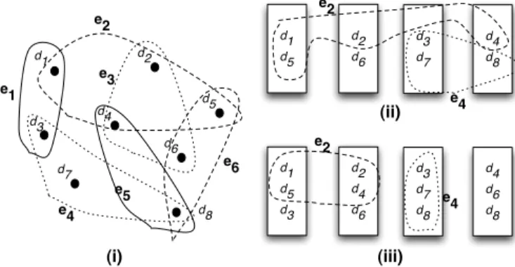
d1 d3 d7 d4 d2 d5 d6 d8 e1 e2 e3 e4 e5 e6 d1 d5 d2 d6 d3 d7 d4 d8 e2 e4 d1 d5 d3 d2 d4 d6 d3 d7 d8 d4 d6 d8 e2 e4 (i) (ii) (iii)
Figure 2: (i) Modeling a query workload as a hypergraph –di denotes the data items, andeidenotes the queries represented as hyperedges; (ii) A layout w/o replication onto 4 partitions – the span of two of the hyperedges is also shown; (iii) A layout with replication – span for both queries reduces by 1.
e ∈ E corresponds to a query in the workload. Figure 2 shows an illustrative example, where we have 6 queries over 8 data items, each of which is represented as a hyperedge over the data items. The figure also shows two layouts of the data items onto 4 partitions of capacity 3 each, without replication and with replication.
Calculating Span:When there is no replication, calculating the span of a query is straightforward since each data item is associated with a single partition. However, if there is replication, the problem becomes NP-Hard. It is essentially identical to theminimum set coverproblem [21], where we are given a collection of subsets of a set (in our case, the partitions) and a query subset, and we are asked to find the minimum number of subsets (partitions) required to cover the query subset.
As an example, for querye2in Figure 2, the span in the first
lay-out is 3. However, in the second laylay-out, we have to choose which of the two copies ofd4to use for the query. Using the first copy (on
second partition) leads to the lowest span of 2. Overall, the average query span for the first layout is 13
6, but use of replication in the
second layout reduces this to86.
We use a standard greedy algorithm for choosing replicas to use for a query and for calculating the span. For each of the partitions, we compute the size of its intersection with the query subset. We choose the partition with the highest intersection size, remove all items from the query subset that are contained in the partition, and iterate until there are no items left in the query subset. This simple greedy algorithm provides the best known approximation to the set cover problem (log|Q|, where|Q|is the query size).
Hypergraph Partitioning:Without replication, the problem we defined above is essentially thek-way (balanced) hypergraph par-titioning problem that has been very well-studied in the literature. However, the optimization goal of minimizing the average span is unique to this setting; prior work has typically studied how to min-imize the number ofcuthyperedges instead. Several packages are available for partitioning very large hypergraphs efficiently [1, 2]. The proposed algorithms are typically heuristics or combinations of heuristics, and most often the source code is not available. We use one such package (hMETIS) as the basis of our algorithms.
Finding Dense Subgraphs of a specified size:Given a set of nodes
Sin a graph, thedensityof the subgraph induced byS is defined to be the ratio of the number of edges in the induced subgraph and
|S|. The dense subgraph problem is to find the densest subgraph of
a given size. To understand the connection to the dense subgraph problem, consider a scenario where we have exactly one “extra” partition for replicating the data items (i.e.,Ne=N−1). Further,
assume that each query refers to exactly two data items, i.e., the hypergraphHis just a graph. One approach would then be to first partition the data items intoN−1partitions without replication, and then try to use this extra partition optimally. To do this, we can construct aresidualgraph, which contains all edges that were cut in this partitioning. The span of each of the queries correspond-ing to these edges is exactly 2. Now, we find the subgraph of size
Csuch that the number of induced edges (among the nodes of the subgraph) is maximized, and we place these data items on the extra partition. The span of the queries corresponding to these edges are all reduced from 2 to 1, and hence this is an optimal way to utilize the extra partition. We can generalize this intuition to hypergraphs and this forms the basis of one of our algorithms.
Unfortunately, the problem of finding the most dense subgraph of a specified size is NP-Hard (with no good worst case approxi-mation guarantees), so we have to resort to heuristics. One such heuristic that we adapt in our work is as follows: recursively re-move the lowest degree node from the residual graph (and all its incident edges) till the size of the residual graph is exactlyC. This heuristic has been analysed by Asahiro et al. [7] who find that this simple greedy algorithm can solve this problem with approxima-tion ratio of approximately2(|VC| −1)(whenC≤ |V|/3).
Sublinear Separators in Graphs:Consider the special case where
His a graph, and further assume that there are only 2 partitions (i.e.,N = 2). Further, lets say that the graph has a small sepa-rator, i.e., a set of nodes whose deletion results in two connected components of size at mostn/2. In that case, we can replicate the separator nodes (assuming there is enough redundancy) and thus guarantee that each query has span exactly 1. The key here is the existence of small separators of bounded sizes. Such separators are known to exist for many classes of graphs, e.g., for any family of graphs that excludes a minor [4].
A separator theorem is usually of the form that, anyn-vertex graph can be partitioned into two setsA,B, such that|A∩B|=
c√nfor some constantc,|A−B|<2n/3,|B−A|<2n/3, and there are no edges from a node inA−Bto a node inB−A. This directly suggests an algorithm that recursively applies the separator theorem to find a partitioning of the graph into as many pieces as required, replicating the separator nodes to minimize the average span. Such an algorithm is unlikely to be feasible in practice, but may be used to obtain theoretical bounds or approximation algo-rithms. For example, we prove that:
THEOREM 1. Let Gbe a graph with n nodes that excludes a minor of constant size. Further, letNe denote the number of
partitions minimally required to hold the nodes ofG(i.e.,Ne = dn/Ce). Then, asymptotically,Ne1.73partitions are enough to
par-tition the nodes ofGwith replication so that each edge is contained completely in at least one partition.
Proof:The proof relies on the following theorem by Alon et al. [4]: THEOREM 2. LetGbe a graph withnnodes that excludes a fixed minor withhnodes. Then we can always find a separation
(A, B)such that|A∩B| ≤h32n 1
2,|A−B|,|B−A| ≤ 2 3n.
Consider a recursive partitioning ofGusing this theorem. We first find a separation ofGintoAandB. SinceAandBare sub-graphs of G, they also exclude the same minor. Hence we can further partitionAandB into two (overlapping) partitions each. Now, both|A|and|B|are≤2
3n+h 3
term is dominated byn, for any > 0. We choose some such
= 1/300. Then, we can write:|A|,|B| ≤(2
3+)n= 0.67nfor
large enoughn.
Now we continue recursively forlsteps getting us2l
subgraphs of the original graphG, such that each of the subgraphs fits in one partition. Note that, by construction, every edge is contained in at least one of these subgraphs; thus2l
partitions are sufficient for data placement as required. Since the partition capacities areO(n), we can use the above formula to computel. We need: 0.67ln < C =n/Ne. Solving forl, we get: l > log2(Ne1.73). Hence, the
number of partitions needed to partitionGwith replication so that each edge is contained in at least one partition is less thanNe1.73.
Although the bound looks strong, note that the above class of graphs can have at mostO(n)edges (i.e., these types of graphs are typically sparse). Proving similar bounds for dense graphs would be much harder and is an interesting future direction.
For general graphs, in Appendix A, we show that:
THEOREM 3. If the optimal solution uses βNe partitions to
place the data items so that each edge is contained in at least one partition, then either we can get an approximation with factor2−2α
for0≤α ≤1usingNepartitions, or a placement using CN2αeβ
partitions with span 1 for each edge.
4.
DATA PLACEMENT ALGORITHMS
In this section, we present several algorithms for data placement with replication, with the goal to minimize the average query span. Instead of starting from scratch, we chose to base our algorithms on existing hypergraph partitioning packages. As we discussed in the previous sections, the problem of balanced and unbalanced hyper-graph partitioning has received a tremendous amount of attention in various communities, especially the VLSI community. Several very good packages are freely available for solving large partition-ing problems [1, 24, 2, 9]. We use a hypergraph partitionpartition-ing al-gorithm (called HPA) as a blackbox in our alal-gorithms, and focus on replicating data items appropriately to reduce the average query span. An HPA algorithm typically tries to find a balanced partition-ing (i.e., all partitions are of approximately equal size) that mini-mizes some optimization goal. Usually, allowing for unbalanced partitions results in better partitioning. In the algorithm descrip-tions below, we assume that the HPA algorithm can return an ex-actly balanced partition, where all partitions are of equal size, if needed.
Following the discussion in the previous section, we develop four classes of algorithms:
• Iterative HPA (IHPA): Here we repeatedly use HPA until all the extra space is utilized.
• Dense Subgraph-based (DS): Here we use a dense subgraph finding algorithm to utilize the redundancy.
• Pre-replication (PR): Here we attempt to identify a set of nodes to replicate a priori, modify the input graph by replicating those nodes, and then run HPA to get a final placement.
• Local Move-based (LM): Starting with a partition returned by HPA, we improve it by replicating a small group of data items at a time.
As expected the space of different variants of the above algorithms is very large. We experimented with many such variants in our work. We begin with a brief listing of some of the key subroutines that we use in the pseudocodes. We then describe a representative set of algorithms that we use in our performance evaluation.
4.1
Preliminaries; Subroutines
The inputs to the data placement algorithm are: (1) the hyper-graph, H(V, E), with vertex set V and (hyper)edge set E that captures the query workload, and (2) the number of partitions,N
and (3) the capacity of each partitionC. We useNeto denote the
minimum number of partitions needed to partition the hypergraph (Ne≤N).
Our algorithms use a hypergraph partitioning algorithm (HPA) as a blackbox. HPA takes as input the hypergraph to be partitioned, the number of partitions, and anunbalance factor(UBfactor). The unbalance factor is set so that HPA has the maximum freedom, but the number of nodes placed in any partition does not exceed C. For instance, if|V|=Ne×Cand if HPA is asked to partition into
Nepartitions, then the unbalance factor is set to be the minimum.
However, if HPA is called withN0 > Ne partitions, then we
ap-propriately set the unbalance factor to the maximum possible. The formula we use in our experiments to set unbalance factor is:
U Bf actor= 100∗partitionCapacity∗noP artitions−totalItems totalItems∗noP artitions
We modify the output of HPA slightly to ensure that the partition capacity constraints are not violated. This is done as follows: if there is a partition that has higher than maximum number of nodes, we move a small group of nodes to another partition with fewer than maximum number of nodes. We use one of our algorithms developed below (LMBR) for this purpose.
In the pseudocodes shown, apart from HPA, we also assume ex-istence of the following subroutines:
• getSpanningPartitions(G, e): Let the current placement (dur-ing the course of the algorithm) beG ={G1,· · ·, GN}where
G1,· · ·, Gndenote the subgraphs ofGassigned to the different
partitions and may not be disjoint (i.e., same node may be con-tained in two or more partitions because of replication). Given a hyperedgee, this procedure finds a minimal subset of the par-titionsM De ⊆ G, such that every node ineis contained in at
least one partition inM De. We use the greedy Set Cover
algo-rithm for this purpose. We start with the partitionGithat has the
maximum overlap withe, and include it inM De. We then
re-move all the nodes inethat are contained inGi(i.e., “covered”
byGi) and repeat till all nodes are covered.
• getQuerySpan(G, e):Given a current placement{G1,· · ·, GN}
and a hyperedgee, this procedure finds the span of the hyper-edgee. We use the same algorithm as above, but return|M De|
instead ofM De.
• getAccessedItems(G, e, g ∈ G): Given a current placement
G = {G1,· · ·, GN}, a hyperedgee and a partition g ∈ G,
this returns the set of items that the query corresponding toe
would access from partitiong, as computed by the greedy Set Cover algorithm. This may be empty even ife∩g6=φ.
• pruneHypergraphBySpan(G,H, minSpan):Given a current placementGand a value ofminSpan, this routine removes all hyperedges fromHwith span less than or equal tominSpan.
• getKDensestNodes(H, K):Given a hypergraphH, this proce-dure returns a dense subgraph containing at nodes having total weight of atmostK. We use a greedy algorithm for this pur-pose: we find the lowest degree node and remove that node and all edges incident on it; if the graph still has nodes having total weight more thanK, we repeat the process by finding the lowest degree node in the new graph.
• pruneHypergraphToSize(H, K): Given a current placement
for getKDensestNodes to find a (dense) hypergraph over nodes having total weight ofK.
• totalWeight(V,Wv):Given a set of verticesV and weight vec-tor of verticesWv, v ∈V, this routine returns the total weight
of vertices.
We note that, because of the modularized way our framework is designed, we can easily use different, more efficient algorithms for solving these subproblems.
4.2
Iterative HPA (IHPA)
Here, we start by using HPA to get a partitioning of the data items into exactlyNepartitions (recall thatNeis the minimum number of
partitions needed to store the data items). We then prune the orig-inal hypergraphH(V, E)to get a residual hypergraphH0(V0, E0)
as follows: we remove all hyperedges that are completely contained in a single partition (i.e., hyperedges with span 1), and we then re-move all the data items that are not contained in any hyperedge. If the number of nodes in theH0
is less than(N−Ne)C(i.e., if the data items fit in the remaining empty partitions), we apply HPA to obtain a balanced partitioning ofH0
and place the partitions on the remaining partitions. This process is repeated if there are still empty partitions.
If the number of nodes inH0
is larger than the remaining capac-ity, we prune the graph further by removing the hyperedges with the lowest span one at a time (these hyperedges are likely to see the least improvement by replication) and the data items that now have 0 degree, until the number of nodes inH0
becomes sufficiently low; then we apply HPA to obtain a balanced partitioning ofH0
and place the partitions on the remaining partitions. If there are still empty partitions, we repeat the process by reconstructing a new residual graph. Algorithm 1 depicts the pseudocode for this technique.
Algorithm 1Iterative HPA (IHPA)
Require: H(V, E), N, C
1: Run HPA to get an initial partitioning into Ne partitions: G = {G1, G2, . . . , GNe};
2: edgeCost=avgDataItemsPerQuery(H); 3: whileedgeCost6= 0and|G| 6=Ndo
4: H0(V0, E0) =pruneHypergraphBySpan(G,H, edgeCost); 5: Ncur= totalW eight(V0,Wv0) C ; 6: if|G|+Ncur≤Nand|H 0 | 6= 0then 7: G=G ∪HPA(H0, Ncur);
8: else if|G|+Ncur> Nthen
9: G=G ∪HPA(H0, N− |G|); 10: else
11: decrementedgeCostby1;
12: end if
13: end while
14: return final partitionsG1, G2,· · ·, GN
4.3
Dense Subgraph-based (DS)
This algorithm directly follows from the discussion in the pre-vious section. As above, we use HPA to get an initial partitioning. We then fill the remainingN−Nepartitions one at a time, by
iden-tifying a dense subgraph of the residual hypergraph. This is done by removing the lowest degree nodes fromH0
until the number of nodes in it reachesC(the partition capacity). These data items are then placed on one of the remaining partitions, and the procedure is repeated until all partitions are utilized. Pseudocode is shown in Algorithm 2.
Algorithm 2Dense Subgraph-based (DS)
Require: H(V, E), N, C
1: Run HPA to get an initial partitioning into Ne partitions: G = {G1, G2, . . . , GNe}; 2: H0 =H; 3: while|G| 6=Ndo 4: H0=pruneHypergraphBySpan(G,H,1); 5: if|H0|= 0then 6: break; 7: end if
8: denseN odes= getKDensestNodes(H0, C); 9: Add a partition containingdenseN odestoG; 10: end while
11: return final partitionsG1, G2,· · ·, GN
4.4
Pre-Replication-based Algorithm (PRA)
This algorithm is based on the idea of identifying small separa-tors and replicating them. However, we do not directly adapt the recursive algorithm described in Section 3 for two reasons. First, since we have a fixed space budget for replication, we must some-how distribute this budget to the various stages and it is unclear how to do that effectively. More importantly, the basic algorithm of bisecting a graph and then recursing is not considered a good approach for achieving good partitioning [37, 25].We instead propose the following algorithm. We start with a partitioning returned by HPA, and identify “important” nodes such that by replicating these nodes, the average query span would be reduced the most. Then, we create a new hypergraph by replicating these nodes (until we have enough nodes to fill all the partitions), and run HPA once again to attain a final partitioning. However, neither of these steps is straightforward.
Identifying Important Nodes: The goal is to decide which nodes will offer the most benefit if replicated. We start with a partitioning obtained using HPA, and then analyze the partitions to decide this. We describe the intuition first. Consider a nodeathat belongs to some partition Gi. Now count the number of those hyperedges
that containabut do not contain any other node inGi; we denote
this number byscorea. If this number is high, then the node is a
good candidate for replication since replicating the node is likely to reduce the query spans for several queries. We use the partitioning returned by HPA to rank all the nodes in the decreasing order by this count, and then process the nodes one at a time.
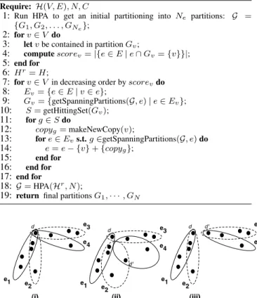
Replicating Important Nodes: Letdbe the node with the high-est value ofscoredamong all nodes. We now have to decide how
many copies ofd to create, and more importantly, which copies to assign to which hyperedge. Figure 3(ii) illustrates the problems with an arbitrary assignment. Here we replicate the nodedto get one more copyd0, and then we assign these two copies to the hyper-edgese1, e2, e3, e4 as shown (i.e., we modify some of the
hyper-edges to removedand addd0 instead). However, the assignment shown is not a good one for a somewhat subtle reason. Sincee1
ande3 (which are assigned the originald) do not share any other
nodes, it is likely that they will span different sets of partitions, and one of them is likely to still pay a penalty for noded. On the other hand, the assignment shown in Figure 3(iii) is better because here the copies are assigned in a way that would reduce the average query span.
We formalize this intuition in the following algorithm. For node
d, letEd={ed1, ed2,· · ·, edk}denote the set of hyperedges that
containd. For hyperedgeedi, letGdi denote the set of partitions
thatedispans. We then identify a set of partitions,S, such that each
Algorithm 3Pre-replication-based Algorithm (PRA)
Require: H(V, E), N, C
1: Run HPA to get an initial partitioning into Ne partitions: G = {G1, G2, . . . , GNe};
2: forv∈V do
3: letvbe contained in partitionGv;
4: computescorev=|{e∈E|e∩Gv={v}}|;
5: end for
6: Hr=H;
7: forv∈V in decreasing order byscorevdo
8: Ev={e∈E|v∈e}; 9: Gv={getSpanningPartitions(G, e)|e∈Ev}; 10: S=getHittingSet(Gv); 11: forg∈Sdo 12: copyg=makeNewCopy(v); 13: fore∈Evs.t.g∈getSpanningPartitions(G, e)do 14: e=e− {v}+{copyg}; 15: end for 16: end for 17: end for 18: G=HPA(Hr, N);
19: return final partitionsG1,· · ·, GN
d e1 e2 e3 e4 d e1 e2 e3 e4 d' d e1 e2 e3 e4 d'
(i) (ii) (iii)
Figure 3: When replicating a node, distribution of the copies to the hyperedges must be done carefully. Distribute the replica copies such that it results in entanglement of the incident hy-peredges.
φ). Such a set is called a “hitting set”. We then replicatedto make a total of|S|copies. Finally, we assign the copies to the hyperedges according to the hitting set, i.e., we uniquely associate the copies ofdwith the members ofS, and for a hyperedgeedi, we assign it
a copy such that the associated element fromSis contained inGdi
(if there are multiple such elements, we choose one arbitrarily). The problem of finding the smallest hitting set is NP-Hard. We use a simple greedy heuristic. We find the partition that is common to the maximum number of setsGdi, include it in the hitting set,
remove all sets that contain it, and repeat. Algorithm 3 depicts the pseudocode for this technique.
4.5
Local Move Based Replication (LMBR)
Finally, we consider algorithms based on local greedy decisions about what to replicate, starting with a partitioning returned by HPA. For simplicity and efficiency, we chose to employ moves in-volving two partitions. More specifically, at each step, we copy a small group of data items from one partition to another. The de-cisions are made greedily by finding the move that results in the highest decrease in the average query span (“benefit”) per data item copied (“cost”). For this purpose, at all times, we maintain a prior-ity queue containing the best moves frompartitionitopartitionj,for alli6=j. For two partitionspartitioni, partitionj, the best
group of data items to be copied frompartitioni topartitionj
is calculated as follows. LetEij = {eij1,· · ·, eijl}denote the
hyperedges that contain data items from both the partitions. We construct a hypergraphHi→j on the data items ofpartitionias
follows: for every edgeeijk, we add a hyperedge toHi→jon the
data items common toeijkandpartitioni. Figure 4 illustrates this
d1 d2 d3 d4 d5 d6 d7 d8 d9 d10 disk1 disk2 d1 d3 d4 d6 e'1 d5 e'2 e'3 e'6 e'4 e'5 H1➔2 Hyperedges spanning
both disk1 and disk2: e1 = {d1, d3, d7, d8, ..} e2 = {d1, d4, d5, d9, ..} e3 = {d5, d8, ..} e4 = {d4, d6, d7, d8, ..} e5 = {d3, d4, d6, d9, ..} e6 = {d6, d9, d10, ..}
Figure 4: Constructing H1→2: e.g., corresponding to hyper-edgee1that spans both partitions, we have a hyperedgee01over
d1andd3.
process with an example.
Now, if we were to copy a group of data itemsXfrompartitioni
topartitionj, the resulting decrease in total span (across all edges)
is exactly the number of hyperedges inHi→jthat are completely
contained inX. Thus, the problem of finding the best move from
partitioni topartitionj is similar to the problem of finding a
dense subgraph, with the main difference being that, we want to minimize the cost/benefit ratio and not maximize the benefit alone. Hence, we modify the algorithm for finding dense subgraph as fol-lows. We first compute the cost/benefit ratio for the entire group of nodes inHi→j. The cost is set to∞if the number of nodes to
be copied is more than the empty space inpartitionj. We then
remove the lowest degree node fromHi→j (and any incident
hy-peredges), and again compute the cost/benefit ratio. We pick the group of items that results in the lowest cost/benefit ratio.
After finding the best moves for every pair of partitions, we choose the overall best move, and copy the data items accordingly. We then recompute the best moves for those pairs which were af-fected by this move (i.e., the pairs containing the destination parti-tion), and recurse until all the partitions are full.
Improved LMBR:Although the above looks like a reasonable al-gorithm, it did not perform very well in our first set of experiments. As described above, the algorithm has a serious flaw. Going back to the example in Figure 4, say we chose to copy data itemd6from
partition1topartition2. In the next step, the same move would
still rank the highest. This is because the construction of hyper-graphH1→2is oblivious to the fact thatd6is also now present in
partition2. Further, it is also possible that, because of replication,
neither of the partitions is actually accessed at all when executing the queries corresponding toe4, e5ore6.
To handle these two issues, during the execution of the algo-rithm, we maintain the exact list of partitions that would be acti-vated for each query; this is calculated using the Set Cover algo-rithm described in Section 3. Now when we consider whether to copy a group of items frompartitionito partitionj, we make
sure that the benefit reflects the actual query span reduction given this mapping of queries to partitions. Pseudocodes for this algo-rithm is give in Algoalgo-rithm 4 and 5.
4.6
3-Way Replication Algorithms
As we have already discussed, many large-scale data manage-ment systems provide default 3-way replication. Here we briefly discuss how the algorithms described above can be modified to han-dle 3-way replication.
PRA-Based 3-Way Replication: We identify PRA the most suit-able algorithm to do this effectively, and modify PRA as follows.
Algorithm 4Improved LMBR
Require: H(V, E), N, C
1: Run HPA to get initial partitionsG = {G1, G2, . . . , GN}intoN
partitions;
2: Compute the set coverM Defor each querye;
3: Initialize PQ (priority queue) to empty; 4: forg=G1toGNdo 5: forg0=G1toGN, g6=g0do 6: PQ.insert(g→g0 ,maxGain(G, g, g0)); 7: end for 8: end for
9: whileall partitions are not fulldo
10: (gsrc→gdest) = PQ.bestMove();
11: copyappropriate items fromgsrctogdest;
12: forg=G1toGN,g6=gdestdo
13: PQ.update(g→gdest, maxGain(G,g, gdest));
14: PQ.update(gdest→g, maxGain(G,gdest, g));
15: end for
16: end while
17: return final partitionsG1,· · ·, GN;
Algorithm 5Improved LMBR maxGain Method
Require: G={G1,· · ·, GN},H(V, E), Gsrc∈ G, Gdest∈ G
1: Esrc={e∈E|getAccessedItems(G, e, Gsrc)6=φ};
2: Edest={e∈E|getAccessedItems(G, e, Gdest)6=φ};
3: E=Esrc∩Edest; 4: if|E| 6= 0then 5: V0=∪e∈EgetAccessedItems(G, e, Gsrc); 6: E0={getAccessedItems(G, e, G src)|e∈E}; 7: create hypergraphH0(V0, E0); 8: Cdest=C− |Gdest|; 9: ifCdest6= 0then 10: H0=pruneHypergraphToSize(H0, Cdest); 11: while|H0|>0do 12: computegain =|E0|/|V0|
13: removelowest degree node fromH0and incident edges;
14: end while
15: end if
16: end if
17: returnthe best value of gain found in the process and the correspond-ingV0;
Because we are interested in replicating all the nodes 3-way, we eliminate the step of finding important nodes from PRA and we replicate each node 3-way by using our “hitting set“ technique to decide which copy must be shared with what hyperedges. PRA ba-sically aims to separate the incident hyperedges in the hypergraph by distributing the copies of nodedsmartly to incident hyperedges.
Simple Distribution Algorithm:In this algorithm, for each node
din the hypergraph we find the set of incident hyperedgesEd. We
assign 3 copies ofdamong|Ed|edges randomly, by assigning
ev-ery|Ed|
3 hyperedges single copy ofd. Only difference between this
algorithm and PRA based 3-way replication algorithm is that PRA based algorithm makes best effort to distribute the copies of noded
among incident hyperedgesEd.
IHPA-Based Algorithm: In IHPA for 3-way replication we run HPA to get partitioning without replication. We remove all the hy-peredges with span 1 from the input graph, and run HPA again on the residual graph to get additional partitions. We repeat this pro-cess one more time to replicate each node exactly 3 times.
4.7
Discussion
We presented four heuristics for data placement with replication. There are clearly many other variations of these algorithms, some of which may work better for some inputs, that can be implemented
quickly and efficiently using our framework and the core operations that it supports (e.g., finding dense subgraphs). In practice, taking the best of the solutions produced by running several of these algo-rithms would guarantee good data placements.
Finally, while describing the algorithms, we assumed a homo-geneous setup where all partitions are identical and all data items have equal size. We have also extended the algorithms to the case of heterogeneous data items. The hMETIS package that we use and also other hypergraph partitioning packages, allow the nodes to have weights. For heterogeneous case the dense subgraph algo-rithm is modified to account for the weights, by removing the node with the lowest value of degree till we have nodes having total spec-ified weight (for both DS and LMBR). Similarly, PRA is modspec-ified by allowing the replication in the original hypergraph such that to-tal weight of replicated nodes is no greater than the sum of all extra available partition capacities. We omit the full details due to lack of space.
5.
EXPERIMENTAL EVALUATION
We are building a trace-driven simulator to experiment with dif-ferent data placement and scheduling policies. The simulator in-stantiates a number of partitions as needed by the experimental setup, uses a data placement algorithm for distributing the data among the partitions, and replays a query trace against it to measure the query span profiles.
We conducted an extensive experimental study to evaluate our algorithms, using several real and synthetic datasets. Specifically, we used the following three datasets:
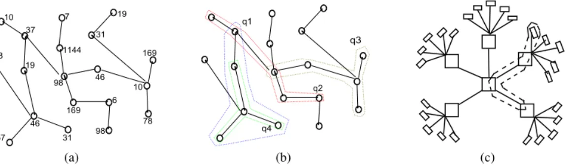
• Random: Instead of generating a query workload completely randomly, we use a different approach to better understand the structure of the problem. We first generate a randomdata item graph of a specified density (edges to nodes ratio). We then randomly generate queries such that the data items in the query form a connected subgraph in the data item graph. For low den-sity data item graphs, this induces significant structure in the query workload that good data placement algorithms can exploit for better performance. Figure 5(a) shows an example data ob-ject graph where the numbers indicate the data item sizes (in MB). Figure 5(b) shows several queries that may be generated using this data item graph – each of the queries forms a con-nected subgraph in the data item graph.
• Snowflake: This is a special case of the above where the data item graph is a tree. This workload attempts to mimic a stan-dard SQL query workload. An example data item graph corre-sponding to the Snowflake dataset is shown in Figure 5(c). Here the large squares indicate the first-level relations, and the small squares indicate the second-level relations. We treat each col-umn of each relation as a separate data item. An SQL query over such a schema that does not contain a Cartesian product corresponds to a connected subgraph in this graph.
• ISPD98 Benchmark Data Sets: In addition to the above synthetic datasets, we tested our algorithms on standard ISPD98 bench-marks [5]. ISPD98 circuit benchmark suite contains 18 circuits ranging from 12,752 to about 210,000 nodes. Hypergraph den-sity (hyperedges to nodes ratio) in all the ISPD98 circuit bench-marks is close to 1, i.e., these graphs are quite sparse. We show results for the first 10 circuit datasets, that contain 12,752 to 69,429 nodes.
We compare the performance of six algorithms: (1)Random, where the data is replicated and distributed randomly, (2)HPA, the base-line hypergraph partitioning algorithm, (3-6) the four algorithms
10 78 37 19 7 1144 19 31 46 98 57 46 31 169 6 98 10 169 78 (a) q1 q2 q3 q4 (b) (c)
Figure 5: (a) An example data item graph; (b) Queriesq1, q2, q3, q4are generated by choosing connected subgraphs of the data item graph; (c) The data item graph corresponding to a Snowflake schema.
hMETIS (HP A) Parameter Values
Parameters value
noP artitions Varies
U Bf actor 1 for almost balanced partitioning, else varies N runs 50 CT ype 2 RT ype 1 V Cycle 1 Reconst 1 dbglvl 0
Table 1:HP AParameter Values
that we propose,IHPA, PRA, DS,andLMBR(Section 4). We use the hMETIS hypergraph partitioning algorithm [24, 1] as our HPA algorithm. For reproducibility, we list the values of the remain-ing hMETIS parameters in Table 1. The experiments were run on a Intel Core2 Duo CPU 2.10GHz, 4GB RAM, Windows PC run-ning Windows 7. All plotted numbers (except the numbers for the ISPD98 benchmark) are averages over 10 random runs.
The key parameters of the dataset that we vary are: (1)|D|, the number of data items, (2-3)minQuerySizeandmaxQuerySize, the bounds on the query sizes that are generated, (4)NQ, the number of queries, (5)C, the partition capacity, (6)numPartitions (NPar), the number of partitions, and (7)densityof the data item graph (defined to be the ratio of the number of edges to the number of nodes). The default values were:|D|= 1000, minQuerySize = 3, maxQuerySize = 11, NQ = 4000, C = 50, NPar = 40, and density = 20.
In several of the plots, we also show the average number of data items per query, denotedADI.
5.1
Random Dataset
We begin with showing the results for the Random dataset with homogeneous data items.
Increasing Number of Partitions (N D): First, we run experiments with increasing the number of partitions. With the default parame-ters, a minimum of 20 partitions are needed to store the data items. We increase the number of partitions from 20 to 45, and compute the average query spans, and average execution times, for the six algorithms over 10 runs. Figures 6(a), and 6(b) show the results of the experiment. HPA does not do replication, and hence the corre-sponding plot is a straight line. The performance of the rest of the algorithms, including Random, improves as we allow for replica-tion. Among those, LMBR performs the best, with IHPA a close second. We saw this behavior consistently across almost all of our experiments (including the other datasets). LMBR’s performance
does come with a significantly higher execution times as shown in Figure 6(b). This is because LMBR tends to do a lot of small moves, whereas the other algorithms tend to have a small num-ber of steps (e.g., DS runs the densest subgraph algorithm a fixed number of times, whereas PRA only has three phases). Since data placement is a one-time offline operation, the high execution time of LMBR may be inconsequential compared to the reduction in query spanit guarantees.
Increasing Query Size (ADI): Second, we vary the number of data items per query from 2 to 10 (by setting minQuerySize = max-QuerySize), choosing the default values for the other parameters. As expected (Figure 6(c)), the average span increase rapidly as the query size increases. The relative performance of the different al-gorithms is largely unchanged, with LMBR and IHPA performing the best.
Increasing Number of Queries (N Q): Next, we vary the number of queries from 1,000 to 11,000, thus increasing the density of the hypergraph (Figure 6(d)). The average query span increases rapidly in the beginning and much more slowly beyond 5,000 queries. Once again the LMBR algorithm finds the best solution by a significant margin compared to the other algorithms.
Increasing Data Item Graph Density: Finally, we vary the data item graph density while from 2 (very sparse) to 20 (dense). The number of partitions was set to 40. As we can see in Figure 6(e), for low density graphs, the average span of the queries is quite low, and it increases rapidly as the density increases. Note that the average query size did not change, so the performance gap is entirely because of the structure of the query hypergraph for low density data item graphs. Further, we note that the curves flatten out as the density increases, and don’t change significantly beyond 10, indicating that the query workload essentially looks random to the algorithms beyond that point.
Overall, our experimental study indicates that LMBR, despite its high running time, should be the data placement algorithm used for minimizing query span/multi-site overheads and energy consump-tion in such scenarios (where we do not have any constraints on the number of replicas that must or can be created).
5.1.1
3-Way Replication
Figures 6(f), 6(g) and 6(h) show a set of experimental results comparing the 3-way replication algorithms that we have discussed in Section 4.6.
Increasing Number of Queries (N Q): Increasing the number of queries, thus increasing the density of the graph, we observe that PRA based 3-way replication algorithm performs the best. This
2.5 3 3.5 4 4.5 5 5.5 20 25 30 35 40 45
Avg Query Span
Number of Partitions |D|=1000, ADI=7, NQ=4000, C=50 HPA Random IHPA PRA DS LMBR (a) 0 100 200 300 400 500 600 20 25 30 35 40 45
Execution Time (seconds)
Number of Partitions |D|=1000, ADI=7, NQ=4000, C=50 HPA Random IHPA PRA DS LMBR (b) 1 2 3 4 5 6 2 3 4 5 6 7 8 9 10
Avg Query Span
Query Size ND=1000, NQ=4000, C=50 HPA Random IHPA PRA DS LMBR Max Query Span
(c) 1.5 2 2.5 3 3.5 4 4.5 5 5.5 0 2000 4000 6000 8000 10000 12000
Avg Query Span
No of Queries ND=1000, ADI=7, NQ=4000, C=50, maxSpan=7 HPA Random IHPA PRA DS LMBR (d) 1 1.5 2 2.5 3 3.5 4 4.5 5 5.5 0 2 4 6 8 10 12 14 16 18 20
Avg Span Per Query
Density |D|=1000, ADI=7, C=50, NPar=40 HPA Random IHPA PRA DS LMBR (e) 1.5 2 2.5 3 3.5 4 4.5 5 5.5 0 2000 4000 6000 8000 10000 12000
Avg Query Span
No of Queries ND=1000, ADI=7, NQ=4000, C=50, maxSpan=7, RF=3, NPar=60 HPA Random SDA PRA3Way (f) 1 2 3 4 5 6 1 2 3 4 5 6 7 8 9 10
Avg Query Span
Query Size ND=1000, NQ=4000, C=50, RF=3, NPar=60 HPA Random SDA PRA3Way (g) 1 1.5 2 2.5 3 3.5 4 4.5 5 5.5 0 2 4 6 8 10 12 14 16 18
Avg Span Per Query
Density |D|=1000, ADI=7, C=50, NPar=60, RF=3 HPA Random SDA PRA3Way (h)
Figure 6:(a)−(e)Results of the experiments on the Random dataset with homogeneous data items illustrate the benefits of intelligent data placement with replication; the LMBR algorithm produces the best data placement in almost all scenarios. Note that, for clarity, they-axes for several of the graphs do not start at 0.(f)−(h)3-way replication results with replication factor of each nodeRF = 3.
is in comparison with HPA (no replication), Random 3-way repli-cation and simple distribution algorithm (SDA). As the number of hyperedges increases in the graph average number of hyperedges incident per node also increases. This effects the SDA algorithm, because SDA tries to distribute the 3 copies of the node randomly to the number of hyperedges incident on it. So as average number of incident hyperedges per node increases, it is more likely for SDA to make bad decisions about distribution of replicas among inci-dent hyperedges, hence SDA’s average span increases with number of queries. On the other hand, PRA employshitting settechnique to do a more smarter replica distribution among the incident hy-peredges. Increase in number of queries doesn’t seem to effect the query span for PRA, which indicates the effectiveness of PRA ap-proach. Hence, PRA based technique performs consistently better than SDA in this experiment.
Increasing Query Size (ADI): Query span for all the algorithms increases with an increase in average data items per query. As we saw that density of the hypergraph affects PRA and SDA, where in-crease in density doesn’t affect PRA. In this experiment inin-crease in hyperedge size doesn’t affect the density of the hypergraph. Hence query span increases for SDA and PRA. PRA again performs con-sistently better than other algorithms.
Increasing Data Item Graph Density: PRA again performs the best compared to Random and SDA when density of the graph is varied. Analysis is similar to what we have discussed before in Section 5.1.
We do not compare with LMBR for this scenario due to its high running time, and because it cannot guarantee the replication con-straint of 3-way replication.
5.2
Snowflake Dataset
Figures 7(a) and 7(b) show a set of experimental results for the Snowflake dataset. Each of the plotted numbers corresponds to an average over 10 random query workloads. The data item graph itself was generated with the following parameters: the number of
levels in the graph was 3, the degree of each relation (the maximum number of tables it may join with) is set to 5, and the number of attributes per table is set to 15. The total number of data items was 2000, requiring a minimum of 20 partitions to store them. Note that we assume homogeneous data items in this case. We plot the average query spans, and the average execution times as the number of partitions increases from 20 to 45.
We also conducted a similar set of experiments with heteroge-neous data item sizes, where we generated TPC-H style queries with data item sizes adhering to the TPC-H benchmark. We chose the scale factor of 25, which means the highest data item size is 28GB and smallest data item size is 25KB. This results in a high skew among the table column sizes. Data item size is calculated as
Size(columnDatatype)∗noRows. The partition capacity was
fixed at 100GB, and we once again plot the average query spans and the average execution times as the number of partitions increases from 20 to 45. The results are shown in Figures 8(a) and 8(b).
Our results here corroborate the results on the Random dataset. We once again see that LMBR performs the best, finding signif-icantly better data layouts than the other algorithms. The perfor-mance differences are quite drastic with homogeneous data item sizes – with 45 partitions, LMBR is able to achieve an average query span of just 1.5, whereas the baseline HPA results in an av-erage span of 3.5. However, we observe that with heterogeneous data item sizes, the advantages of using smart data placement algo-rithms are lower. With an extreme skew among the data item sizes, the replication and data placement choices are very limited.
5.3
ISPD98 Benchmark Dataset
Finally, Figure 9 shows the comparative results for first ten of hy-pergraphs from the ISPD98 Benchmark Suite, commonly used in the hypergraph partitioning literature. The number of hyperedges in the datasets range from 14111 to 75196 and number of nodes range from 12752 to 69429. Here we set the partition capacity so that exactly 20 partitions are sufficient to store the data items, and we plot the results with number of partitions set to 35. The
1 2 3 4 5 20 25 30 35 40 45
Avg Query Span
Number of Disks |D|=2000, ADI=15, NQ=4000, C=100,
Levels=3, Degree=5, Attrs=15
HPA Random IHPA PRA LMBR DS (a) 0 100 200 300 400 500 600 700 20 25 30 35 40 45
Execution Time (seconds)
Number of Disks |D|=2000, ADI=15, NQ=4000, C=100,
Levels=3, Degree=5, Attrs=15 HPA Random IHPA PRA LMBR DS (b)
Figure 7: Results of the Experiments on the Snowflake Dataset
2 2.5 3 3.5 4 4.5 5 20 25 30 35 40 45
Avg Query Span
Number of Partitions |D|=1000, ADI=7, NQ=4000, DC=100GB, scaleFactor=25 HPA Random IHPA PRA LMBR DS (a) 0 50 100 150 200 250 300 350 400 20 25 30 35 40 45
Execution Time (seconds)
Number of Partitions |D|=1000, ADI=7, NQ=4000, DC=100GB, scaleFactor=25 HPA Random IHPA PRA LMBR DS (b)
Figure 8: Results of the Experiments on a TPC-H style Bench-mark with unequal data item sizes. The relation sizes were cal-culated assuming a scale factor of 25.
pergraphs in this dataset tend to have fairly low densities, resulting in low query spans. In fact, LMBR is able to achieve an average query span of close to the minimum possible (i.e., 1) with 35 parti-tions. Most of the other algorithms perform about 20 to 40% worse compared to LMBR.
These additional experiments further corroborate our claim that intelligent data placement with replication can significantly reduce the coordination overheads in data centers, and further that our LMBR algorithm outperforms rest of the algorithms significantly.
6.
CONCLUSIONS
In this paper, we solve the combined problem of data placement and replication, given a query workload, to minimize the total re-source consumption and by proxy, the total energy consumption, in very large distributed or multi-site read-only data stores. Directly optimizing for either of these metrics is likely infeasible in most practical scenarios because of the large number of factors involved. We instead identify query span, the number of machines involved in executing a query, as having a direct and significant impact on the total resource consumption, and focus on minimizing the av-erage query span for a given query workload. We formulated and analyzed the problems of data placement and replica selection for this metric, and drew connections to several well-studied graph the-oretic concepts. We used these connections to develop a series of algorithms to solve this problem, and our extensive experimental evaluation over several datasets demonstrated that our algorithms can result in drastic reductions in average query spans. We are planning to extend our work in several different directions. As we discussed earlier, we believe that temporal scheduling algorithms can be used to correct the load imbalance that may result from opti-mizing for query span alone; although analysis tasks are usually not
0 0.5 1 1.5 2 2.5 3 3.5 4 4.5
ibm01 ibm02 ibm03 ibm04 ibm05 ibm06 ibm07 ibm08 ibm09 ibm10
Avg Query Span
ISPD98 Benchmark numPartitions=35 ADI HPA Random IHPA PRA DS LMBR
Figure 9: Results of the experiments on the first 10
hy-pergraphs, ibm01, . . . , ibm10, from the ISPD98 Benchmark Dataset
latency sensitive, there are still often deadlines that need to be sat-isfied. We plan to study how to incorporate such deadlines into our framework. We are also planning to study how to efficiently track changes in the query workload nature online, and how to adapt the replication decisions online.
7.
ADDITIONAL AUTHORS
8.
REFERENCES
[1] hMETIS: A hypergraph partitioning package,
http://glaros.dtc.umn.edu/gkhome/metis/hmetis/overview. [2] MLPart,
http://vlsicad.ucsd.edu/gsrc/bookshelf/slots/partitioning/mlpart/. [3] A. Abouzeid, K. Bajda-Pawlikowski, D. Abadi, A. Silberschatz, and
A. Rasin. HadoopDB: an architectural hybrid of mapreduce and dbms technologies for analytical workloads.PVLDB, August 2009. [4] N. Alon, P. D. Seymour, and R. Thomas. A separator theorem for
graphs with an excluded minor and its applications. InSTOC, 1990. [5] C. J. Alpert. The ISPD98 circuit benchmark suite. InProc. of Intl.
Symposium on Physical Design, 1998.
[6] H. Amur, J. Cipar, V. Gupta, G. Ganger, M. Kozuch, and K. Schwan. Robust and flexible power-proportional storage. InSoCC, 2010. [7] Y. Asahiro, K. Iwama, H. Tamaki, and T. Tokuyama. Greedily
finding a dense subgraph. InSWAT, 1996.
[8] R. B. Boppana. Eigenvalues and graph bisection: An average-case analysis. InFOCS, 1987.
[9] A. E. Caldwell, A. B. Kahng, and I. L. Markov. Design and implementation of move-based heuristics for VLSI hypergraph partitioning.J. Exp. Algorithmics, 5:5, 2000.
[10] M. M. M. K. Chowdhury, M. Zaharia, J. Ma, M. I. Jordan, and I. Stoica. Managing data transfers in computer clusters with orchestra. InSIGCOMM, pages 98–109, 2011.
[11] D. Colarelli and D. Grunwald. Massive arrays of idle disks for storage archives. InSupercomputing, 2002.
[12] C. Curino, E. P. C. Jones, R. A. Popa, N. Malviya, E. Wu, S. Madden, H. Balakrishnan, and N. Zeldovich. Relational cloud: a database service for the cloud. InCIDR, pages 235–240, 2011. [13] C. Curino, Y. Zhang, E. P. C. Jones, and S. Madden. Schism: a
workload-driven approach to database replication and partitioning.
PVLDB, 3(1):48–57, 2010.
[14] J. Dittrich, J.-A. Quiané-Ruiz, A. Jindal, Y. Kargin, V. Setty, and J. Schad. Hadoop++: making a yellow elephant run like a cheetah (without it even noticing).PVLDB, 3:515–529, September 2010. [15] Z. Du, J. Hu, Y. Chen, Z. Cheng, and X. Wang. Optimized qos-aware
replica placement heuristics and applications in astronomy data grid.