UCLA
UCLA Electronic Theses and Dissertations
Title
Deep Generative Classifier with Short Run Inference Permalink https://escholarship.org/uc/item/8kx4z8qw Author Fischer, Eric Publication Date 2020 Peer reviewed|Thesis/dissertation
UNIVERSITY OF CALIFORNIA Los Angeles
Deep Generative Classifier with Short Run Inference
A thesis submitted in partial satisfaction of the requirements for the degree Master of Science in Computer Science
by
Eric Mercado Fischer
c
Copyright by Eric Mercado Fischer
ABSTRACT OF THE THESIS
Deep Generative Classifier with Short Run Inference
by
Eric Mercado Fischer
Master of Science in Computer Science University of California, Los Angeles, 2020
Professor Song-Chun Zhu, Chair
A deep generative classifier employs Short Run Markov Chain Monte Carlo inference with Langevin dynamics and backpropagation through time. In contrast to a convolutional neural network (ConvNet) with analogous architecture, the Short Run classifier approaches the same classification accuracy and (1) may synthesize data, (2) may learn unsupervised from additional unannotated data, and (3) exhibits robustness to adversarial attacks, due to the stochasticity of the Langevin equation and the top-down architecture of the generator network. The ConvNet classifier lacks the ability to perform (1) or (2) and possesses no defense against adversarial attacks, a critical concern for any deployed machine learning system. Meanwhile, the Short Run classifier demonstrates the capacity to improve in both classification accuracy and the quality of data synthesis, given additional unannotated data.
The thesis of Eric Mercado Fischer is approved.
Mark Stephen Handcock Demetri Terzopoulos
Song-Chun Zhu, Committee Chair
University of California, Los Angeles 2020
To my parents
TABLE OF CONTENTS
1 Introduction . . . 1
1.1 Convolutional Neural Network . . . 3
1.2 Generator Network . . . 4
1.3 Alternating Backpropagation . . . 6
1.4 Short Run MCMC . . . 7
2 Prior Art. . . 11
3 Deep Generative Classifier . . . 14
3.1 Model . . . 14
3.2 Learning . . . 15
3.3 Short Run Inference . . . 16
3.4 Learning with Short Run Inference . . . 18
3.5 Objective and Estimating Equation . . . 19
3.6 Backpropagation through Time . . . 19
3.7 Algorithm . . . 20 4 Experiments . . . 23 4.1 SVHN Dataset . . . 24 4.2 Qualitative Results . . . 25 4.3 Quantitative Results . . . 27 4.4 Classification . . . 28 4.5 Adversarial Robustness . . . 29
5 Conclusion . . . 33
A Appendix . . . 34
A.1 Model Architectures . . . 34
LIST OF FIGURES
4.1 Synthesized samples using 40,000, 80,000, and 120,000 training examples . . . 25
4.2 Reconstructed samples using 40,000, 80,000, and 120,000 training examples . . . 26
4.3 Reconstructed samples in which each row represents a digit . . . 27
4.4 Effect of adversarial attack on ConvNet and Short Run classifiers . . . 31
LIST OF TABLES
4.1 MSE and FID using 40,000, 80,000, and 120,000 training examples . . . 28
4.2 Classification accuracy using 40,000, 80,000, and 120,000 training examples . . . 29
A.1 Generator network structure . . . 34
A.2 Small classifier network structure . . . 35
ACKNOWLEDGMENTS
I would like to thank my advisors Dr. Song-Chun Zhu and Dr. Ying Nian Wu for their enthusiastic teaching and inspiration. They offer a wealth of knowledge, and I am fortunate and motivated to continue learning from them during my Statistics Ph.D. program.
I am thankful to Dr. Mark Handcock both for showing me the wonderful world of Monte Carlo methods and for serving as a member on my committee. I am thankful to Dr. Demetri Terzopoulos for introducing me firsthand to his monumental work in computer vision and for serving on my committee.
I am also grateful to the many Computer Science, Statistics, and Philosophy professors at UCLA from whom I have learned and will continue to learn in the next few years. I thank the faculty as well and Juliana Alvarez in particular for her terrific advising.
I could not have done this without Joanne, who helped me care for my basset hound Puppy this spring.
Last but certainly not least, I am exceptionally grateful to Erik Nijkamp, whose guidance and encouragement has far exceeded what anyone could expect from a fellow student. I only hope that I may have a similar impact for students seeking knowledge from me.
CHAPTER 1
Introduction
Introduced in this study is a deep generative classifier employing Short Run Markov Chain Monte Carlo (MCMC) inference with Langevin dynamics and backpropagation through time (BPTT). As the Short Run classifier uses a generator network and Short Run MCMC infer-ence based on the alternating backpropagation algorithm, the generator network is defined in Section 1.2, the alternating backpropagation algorithm in Section 1.3, and Short Run MCMC inference in Section 1.4.
The generator network is a top-down convolutional neural network (ConvNet, or CNN). ConvNets are introduced in Section 1.1, including a bottom-up ConvNet classifier used as a reference in this study. The network architectures of a generator network and small classifier that compose the Short Run classifier are given in Appendices A.1 and A.2, respectively. The network architecture of the ConvNet classifier is given in Appendix A.3.
The Short Run classifier components, i.e., the generator network and small classifier, with some minor modifications may be combined to form the ConvNet classifier. The four transpose convolutional layers of the generator network become convolutional layers in the ConvNet classifier, with the order of layers reversed. As shown in Appendix A, the generator network receives as input a 200-dimensional latent variable z and transforms the number of output feature maps, or channels, in the following order: 200, 128, 128, 64, and 3. The ConvNet classifier receives as input a 3-by-28-by-28 pixel imagexand transforms the number of output channels in the following order: 3, 64, 128, 128, and 200, i.e., the reverse. Excluding two max pooling layers and a flattening layer, the three remaining layers of the ConvNet
classifier are identical to the three layers of the small classifier.
With the analogous architectures of the Short Run and ConvNet classifiers, the Short Run classifier has a fair discriminative model with which it can be compared. As the models have roughly the same expressive capacity, any difference in learning outcomes can be at-tributed to the different learning algorithms. The Short Run classifier approaches the same classification accuracy and (1) may synthesize data, (2) may learn unsupervised from addi-tional unannotated, or unlabelled, data, and (3) exhibits robustness to adversarial attacks, due to the stochasticity of the Langevin equation and the top-down architecture of the gen-erator network. The ConvNet classifier lacks the ability to perform (1) or (2) and possesses no defense against adversarial attacks, a critical concern for any deployed machine learning system. Meanwhile, the Short Run classifier demonstrates the capacity to improve in both classification accuracy and the quality of data synthesis, given additional unannotated data. Inference methods related to Short Run MCMC are discussed in Chapter 2 on Prior Art. The Short Run deep generative classifier is defined in Chapter 3, beginning with the generative model and learning for a generative model defined in Sections 3.1 and 3.2, respectively. Short Run inference and an updated learning algorithm and maximization objective for Short Run inference are defined in Sections 3.3, 3.4, and 3.5, respectively. BPTT for the Langevin dynamics is defined in Section 3.6 before finally the full learning algorithm in Section 3.7.
Experimental results are presented in Chapter 4, beginning with a brief introduction to the Street View House Numbers (SVHN) dataset in Section 4.1. Qualitative and quanti-tative results for the generative model are displayed in Sections 4.2 and 4.3, respectively, before comparing the classification accuracies of the Short Run and ConvNet classifiers in Section 4.4.
The results in Section 4.5 demonstrate the robustness of the Short Run classifier to adversarial attacks. Namely, the Fast Gradient Sign Attack (FGSM) is performed on both classifiers and the Short Run classifier displays nearly 20% better classification accuracy in
response to adversarial perturbations. The conclusion in Chapter 5 summarizes this study.
1.1
Convolutional Neural Network
ConvNets [1, 2] were initially designed for discriminative, bottom-up networks, but input may propagate through a ConvNet architecture in a bottom-up or top-down direction. In the bottom-up direction, convolutional layers effectively perform feature extraction to transform an observed signalxinto an energy−fθ(x). Bottom-up ConvNets are used for discriminative models, such as the ConvNet classifier (A.3) in this study, and energy-based models (EBM), such as the DeepFRAME model [3] and other exponential family models.
An EBM [4, 5, 6, 7, 8, 9] is defined aspθ(x) = Z1(θ)exp(fθ(x)), in whichfθis parameterized by a bottom-up ConvNet and −fθ(x) is the energy function. An EBM may be regarded as the physical analog of a probability distribution. If fθ(x) is linear in θ, it reduces to the exponential family model in statistics or the Gibbs distribution in statistical physics. pθ(x) may be considered an evaluator, in which fθ assigns a value to x, and pθ(x) evaluates x according to a normalized probability distribution [10].
In the top-down direction of a generator network, such as the one (A.1) in this study, transpose convolutional layers transform a latent variable z into a synthesized signal ˆx = gθ(z). A latent variable z encodes, and is meant to explain, an observed signal x. Top-down ConvNets are used for generator networks and other latent variable models, such as independent component analysis and sparse coding [11].
Hence, the family of generative models can be divided into energy-based models, i.e., undirected graphical models, and latent variable models, i.e., directed graphical models, which consists of generator and inference models. [10] performs joint training of energy-based, generator, and inference models in a framework referred to as the divergence triangle. For the bottom-up ConvNet classifier in this study, the objective is to correctly predict a label y with a prediction ˆy, in which ˆy =fθ(x) is a nonlinear transformation of x. f is a
composition ofLlayers, in which each layer consists of a linear mapping and an element-wise nonlinear rectification. This is shown by
x→h(1) →h(l−1) →h(l) → · · · →h(L) →y,ˆ (1.1)
in which h(l) is a d(l)-dimensional vector defined recursively for l = 1, ..., L by
h(l) =f(l)(W(l)h(l−1)+b(l)). (1.2)
Here, h(0) = x and h(L+1) = ˆy, and θ = (W(l), b(l), l = 1, ..., L+ 1). W(l) is the weight matrix, and b(l) is the bias or intercept vector of layer l. f(l) is an element-wise nonlinear transformation, i.e., for v = (v1, ..., vd)>, f(l)(v) = (f(l)(v1), ..., f(l)(vd))>. A commonly used nonlinear rectification is the rectified linear unit (ReLU): f(l)(a) = max(0, a) [12].
A top-down ConvNet, here considered supervised with latent variables h known, trans-forms an initial latent variable h into a signal x, as shown by
h→h(L) →...→h(1) →x, (1.3)
in which h(l) is a d(l)-dimensional vector defined recursively for l =L+ 1, ...,1 by
h(l−1) =g(l)(W(l)h(l)+b(l)). (1.4)
Here, h(L+1) =h and h(0) =x. g(l) is an element-wise nonlinear rectification such as ReLU. The resulting top-down ConvNet may be defined as ˆx = gθ(h), in which θ = (W(l), b(l), l = 1, ..., L+ 1) [12]. Often z is used instead of h to refer to a latent variable; following this convention, the top-down ConvNet may be defined as ˆx=gθ(z).
The generator network uses a top-down ConvNet for unsupervised learning problems with latent variables unknown.
1.2
Generator Network
The generator network [13, 14] is a nonlinear generalization of factor analysis, a prototype model in unsupervised learning that maps latent variables to observed signals. It generalizes
the linear mapping in factor analysis to a nonlinear mapping defined by a top-down ConvNet. Factor analysis may also be generalized with regard to the prior model or prior assumption of the latent variables. This led to models such as independent component analysis, sparse coding, matrix factorization, and nonnegative matrix factorization [11].
The generator network is defined as
x=gθ(z) +,
z ∼ N(0, Id), ∼ N(0, σ2ID), d < D, (1.5)
in which x is a D-dimensional observed data vector such as an image, g is the generator network, θ are the model parameters, z = (zk, k = 1, ..., d) is a d-dimensional vector of con-tinuous latent variables, and is a D-dimensional vector of Gaussian white noise. The prior distribution p(z) is known, such as z ∼ N(0, Id), in which Id stands for the d-dimensional identity matrix. The generator network provides nonlinearity in comparison to the tradi-tional factor analysis model defined asx=W z+, in which W is aD×d matrix. It learns by minimizing the reconstruction error kx −gθ(z)k2 between an observed image x and a synthesized image gθ(z).
Recall the top-down ConvNet structure of the generator network, defined as
z(l−1) =g(l)(W(l)z(l)+b(l)), (1.6)
in which z(l) is the latent variable at layer l, g(l) is an element-wise nonlinearity at layer l, W(l) is the matrix of network weights at layerl,b(l) is the vector of bias terms at layerl, and θ = (W(l), b(l), l= 1, ..., L) are the model parameters at layerl. The top-down ConvNet may be considered a recursion of the original factor analysis model, in which the latent variables at layer l−1 are obtained by a linear superposition of the basis vectors, or functions, that are column vectors of W(l), with the latent variables at layer l serving as coefficients of the superposition [11].
For understanding, the top-down ConvNet (1.6) of the generator network may be imag-ined as a pyramid, in which the top layer, or top of the pyramid, is given a latent variable
z(L) = z, and the bottom layer, or bottom of the pyramid, outputs a synthesized example z(0) = gθ(z) = ˆx. From the top of the pyramid moving downward, the top-down ConvNet transforms a latent variable z into a synthesized example gθ(z) = ˆx.
The generator network has the following motivating properties, none of which can be attributed to the ConvNet classifier used as a reference in this study:
(1) Analysis: The model disentangles variations in observed signals into independent
variations in latent variables.
(2) Synthesis: The model can synthesize new signals by sampling latent variables from their known prior distribution and transforming them into a signal.
(3) Embedding: The model embeds the high-dimensional, non-Euclidean manifold formed by observed signals into a low-dimensional, Euclidean space of latent variables, such that linear interpolation in the latent variable space results in nonlinear interpolation in the data space [11].
In this study, the generator network is learned by Short Run MCMC inference, which is based on the alternating backpropagation algorithm.
1.3
Alternating Backpropagation
The alternating backpropagation algorithm [11] developed for the generator networkgθ(z) is a nonlinear generalization of the alternating regression scheme of the Ruben-Thayer Expec-tation Maximization (EM) algorithm [15, 16], used for learning the factor analysis model. It is a stochastic approximation algorithm that converges to the maximum likelihood esti-mate. The algorithm iterates between an inferential backpropagation step for inferring latent variables and a learning backpropagation step for updating model parameters:
(1) Inferential Backpropagation: For each training example, latent variables are inferred by Langevin dynamics or gradient descent.
(2) Learning Backpropagation: Given the inferred latent variables, model parameters are updated by gradient descent.
For every update of the model parameters in the learning step, an inner loop performs multiple updates of the latent variables with Langevin dynamics or gradient descent in the inferential step. In this step, Langevin dynamics [17] solves an `2-penalized nonlinear least-squares problem to guide the evolution of z over k Langevin steps, such that z may reconstruct x given the current W. Langevin dynamics may be considered a stochastic sampling counterpart of gradient descent [18]. Short Run MCMC inference also has an inner loop each learning iteration for the inference of latent variables.
The inference dynamics of alternating backpropagation create an explain-away inference process, in which the latent variables compete with each other to explain away, i.e., minimize, the current residual x−gθ(z). Both the inferential and learning steps are guided by the residualx−gθ(z), and as a result, the computation of their respective gradients share most of the same chain rule calculations. The updating of the model parameters θ in the learning step and the latent variable z in the inferential step collaborate to reduce the reconstruction error kx −gθ(z)k2 for an example x. Some key advantages of the explain-away inference dynamics of alternating backpropagation and Short Run MCMC inference include:
(1) The latent variables may follow sophisticated prior models, e.g., a dynamic model such as vector auto-regression for textured motions [19] or dynamic textures [20].
(2) The model may learn with incomplete or indirect training data. For example, training images may include occluded regions, and the latent variables can still be obtained and, moreover, used to reconstruct the occluded regions [11].
1.4
Short Run MCMC
Generator networks involve latent variables that follow some prior distribution, such that the marginal distribution of observed examples may be obtained by integrating out the latent
variables. But as this integral is analytically intractable, the learning of generator networks requires an inference method to sample from the posterior distribution of latent variables, pθ(z|x). For this inference, some form of MCMC posterior sampling such as Gibbs sampling [21], Langevin dynamics [17], or Hamiltonian Monte Carlo [22] is often used.
Short Run MCMC [23, 24, 25], employing Langevin dynamics, does not actually sample from the posteriorpθ(z|x) but rather an approximate posterior qθ(z|x). Initialized from the prior z ∼ N(0, Id) and guided by the negative log posterior,−logpθ(z|x), it is a finite-step Langevin flow that may serve as an approximate sampler of the posterior distribution of latent variables.
For each training example, Short Run MCMC initializes a nonconvergent, nonmixing, nonpersistent Markov chain from a prior such as the uniform noise distribution and performs a given number of stepsk, e.g., 20 or 100, of Langevin dynamics toward a target distribution. In this study, the target distribution is −logpθ(z|x), but it may also be an EBM such as in [23], which applies Short Run MCMC to learning the EBM. An EBM,pθ(x) = Z(1θ)exp(fθ(x)), directly specifies the marginal distribution of observed examples,pθ(x), and does not involve any latent variables.
The gradient-based dynamics of Short Run MCMC make it a k-step residual network or recurrent neural network (RNN), which transforms an initial distribution z0 into a learned approximate distribution q. Each learning iteration, a fixed number of Langevin steps k are taken toward the target distribution, such as the current EBM in [23], or the negative log posterior −logpθ(z|x) in this study, and the learned approximate distribution q is fur-ther refined through an update of the parameters θ of the generator network. The learned approximate distribution q is effectively kept across learning iterations, as opposed to the EBM, as in [23], or the true posterior pθ(z|x), as in this study, that only serves as the guide and is discarded.
The only purpose, then, of the target distribution, such as the EBM or −logpθ(z|x), at any given learning iteration is to guide the k-step Langevin dynamics. To update the
gen-erator parameters θ, the difference between synthesized examples, produced by the k-step Langevin flow, and observed examples is calculated to perform an update based on the maxi-mum likelihood learning gradient, as if the synthesized samples were true samples of the tar-get distribution, although again they are samples from an approximate distributionq. In the case of learning the posterior distribution of latent variables, pθ(z|x), the learning objective becomes both to minimize the Kullback-Leibler (KL) divergence between the approximate and posterior distributions, KL(qθ(z|x)kpθ(z|x)), and to maximize the data log-likelihood L(θ) = n1Pn
i=1logpθ(xi) as in usual maximum likelihood estimate (MLE) learning. With this objective, the synthesized examples eventually come to match the observed examples in terms of some statistical properties defined by the model [23].
Short Run MCMC, then, unlike traditional research in EBM and MCMC methods, does not adopt the traditional goal of learning an EBM with convergent MCMC. As a result of relinquishing this goal, it is liberated from the pursuit of traditionally sought-after MCMC properties, such as convergence, mixing, and persistence. Although typically undesirable, the nonconvergence, nonmixing, and nonpersistence exhibited by Short Run MCMC may actually be regarded as beneficial, as it allows for greatly reduced computational expense while not compromising learning integrity. It is easy to motivate the rationale of Short Run MCMC in giving up these MCMC properties:
(1) Convergence to an EBM using MCMC may be impractical, especially if the energy function is multimodal, as is the case with natural images.
(2) For a multimodal EBM, MCMC usually does not mix. MCMC chains from different starting points typically get trapped in different local modes, as opposed to traversing modes and mixing with each other to discover more of the landscape.
(3) Nonpersistent MCMC, by eschewing the requirement that Markov chains should have some nonzero probability of returning to a previous state, is less computationally expensive and more convenient [23].
In the alternating backpropagation algorithm, persistent MCMC chains are used, i.e., the Langevin dynamics is initialized from the values of the latent variables at the end of the previous learning iteration. Although inspired by alternating backpropagation, Short Run MCMC differs in this fundamental regard by design.
CHAPTER 2
Prior Art
A prominent alternative to MCMC posterior sampling for the inference of latent variables is variational inference, as is used in the variational autoencoder (VAE) [14]. Variational inference methods employ a simple factorized distribution to approximate the posterior dis-tribution of latent variables. These methods assume, for each observed example, an approx-imate posterior with variational parameters specific to the example. These parameters may be optimized by minimizing the Kullback-Leibler divergence between the approximate and true posterior distributions of the latent variables.
To perform inference, VAE uses an extra inference network that maps each input example to a mean vector and diagonal variance-covariance matrix of the approximate multivariate Gaussian posterior distribution of the latent variables. Despite its success, VAE has the following disadvantages:
(1) VAE does not perform explicit explain-away inference of the latent variables.
(2) To perform inference, VAE employs an extra inference network with a separate set of parameters, adding to both computational expense and model complexity.
(3) The design of the extra inference network is not automatic and may be difficult, especially if the corresponding generative model has multiple layers of latent variables.
In a deep generative model with one layer of latent variables at the top layer, such as the one in this study, designing the VAE inference network may be challenging but within reason. In a multi-layer generative model with multiple layers of bottom-up and top-down interactions, it may be exceedingly difficult. Short Run MCMC inference, on the other hand,
does not require the design of an extra inference network and is unchanged even for models with multiple layers of latent variables [25].
Another successful approach for training the generator network is the Generative Ad-versarial Network (GAN) [13], which also uses an extra network with a separate set of pa-rameters. In the GAN, a discriminator network plays an adversarial role in a game against the generator network as a means to train the generator. Compared to Short Run MCMC inference that performs explicit explain-away inference of the latent variables and VAE that infers the latent variables with the help of an assisting network, GAN uses this learning algorithm to avoid the inference of latent variables altogether.
In comparison to the VAE and GAN, Short Run MCMC inference is simpler and less computationally expensive. Taking the place of the inference network in VAE is only a noise-initialized, finite-step Langevin flow that adds no extra parameters to the model other than the few required for tuning the Short Run inference dynamics [25]. The explain-away inference of alternating backpropagation also lead to better learning from incomplete or indirect data, which may be difficult or inconvenient for VAE and GAN [11]. Short Run MCMC inference, furthermore, outperforms the VAE with regard to data reconstruction and synthesis [25].
As mentioned, Short Run MCMC introduced by Nijkamp, Hill, et al. [23] is unique amongst research in EBM and MCMC by not adopting the traditional goal of learning an EBM with convergent MCMC. Although Short Run MCMC is not a valid sampler of the EBM, it is indeed a valid model for the data in terms of matching statistics of the data distribution, and arguments can be found in [23]. Grenander [26] referred to maximum likelihood learning of the EBM as an “analysis by synthesis” scheme. Various works that parameterize the energy function of the EBM with a ConvNet, including works using Short Run MCMC, have shown that the “analysis by synthesis” scheme generates highly realistic images [23, 27, 28].
[29], in which MCMC samples are initialized from observed data. Data initialization meth-ods such as CD are often called “looking-forward” methmeth-ods, as samples are initialized from the latent space to which they are intended to converge. There are also persistent initializa-tion methods, often called “falling-behind” methods, in which the the MCMC samples are initialized from the values of the latent variables at the end of the previous learning iteration. Persistent CD [30] was then introduced as a generalization of CD.
All CD frameworks seek to learn the EBM, whereas Short Run MCMC does not retain a learned EBM but only a learned approximate distribution. In contrast to Persistent CD, Short Run MCMC is less computationally expensive and more convenient due to MCMC nonpersistence [23]. In contrast to MCMC methods that use persistent initialization in general, Short Run MCMC differs in this fundamental regard by design. Short Run MCMC has also been used to investigate the anatomy of MCMC-based maximum likelihood learning of the EBM in [24] and to learn deep generative models with one or more layers of latent variables organized in top-down architectures in [25].
As of yet, there is no prior art using Short Run MCMC for a deep generative classifier, or with backpropagation through time. However, the alternating backpropagation algorithm has indeed been used to perform BPTT in [20], which uses a dynamic generator model for spatial-temporal processes such as dynamic textures and action sequences.
CHAPTER 3
Deep Generative Classifier
A deep generative model [31, 32, 33] consists of one or more layers of latent variables orga-nized in a top-down architecture (1.6). Learning such a model requires, for each example x, the inference of a latent variable z based on the posterior distribution of latent variables, pθ(z|x), for which MCMC posterior sampling is often used.
Short Run MCMC sampling does not sample from the posterior pθ(z|x) but rather an approximate posterior qθ(z|x), in a Short Run learning algorithm discussed in greater detail beginning in Section 3.4. First, the generative model, learning, and Short Run inference are introduced.
3.1
Model
Let x be an observed example, such as an image, and let z be the corresponding latent variable.
(1) The joint distribution of (x, z) is pθ(x, z), in which θ are model parameters. (2) The marginal distribution ofx is pθ(x) =R pθ(x, z)dz.
(3) Givenx, z may be inferred based onposteriordistribution pθ(z|x) = pθ(x, z)/pθ(x). Recall the generator network gθ(z), a top-down ConvNet, used in this study:
x=gθ(z) +,
in which x is a D-dimensional observed data vector such as an image, g is the generator network, θ are the model parameters, z = (zk, k = 1, ..., d) is a d-dimensional vector of con-tinuous latent variables, and is a D-dimensional vector of Gaussian white noise. The prior distribution p(z) is known, such as z ∼ N(0, Id), in which Id stands for the d-dimensional identity matrix.
For the generator network, pθ(x, z) is such that [x|z]∼ N(gθ(z), σ2ID), in whichD is the dimensionality of x. Hence, the log-joint distribution of the model is defined as
logpθ(x, z) = log[p(z)pθ(x|z)] (3.1) = −1
2[kzk 2
+kx−gθ(z)k2/σ2] +c, (3.2)
in which cis a constant independent of θ.
Intuitively, with this distribution, (1) the generator parameters θ may be learned such that the reconstruction error kx−gθ(z)k2 is minimized, and (2) z may be regularized, i.e., learned such that kzk2 is minimized.
Learning and inference may be accomplished by maximizing the complete-data log-likelihood logpθ(x, z), but it is more rigorous to maximize the observed-data log-likelihood L(θ) = n1 Pn
i=1logpθ(xi) = n1
Pn
i=1log
R
pθ(xi, zi)dzi (3.3), which takes into account uncer-tainties in inferring z.
3.2
Learning
Let pdata(x) be the data distribution that generates the observed example x. The learn-ing of the parameters θ of pθ(x) may be based on minθKL(pdata(x)kpθ(x)). KL(pkq) = Ep[log(p(x)/q(x))] is the KL divergence from p toq.
may be approximated by maximizing the observed-data log-likelihood, L(θ) = 1 n n X i=1 logpθ(xi), (3.3)
which lends the maximum likelihood estimate (MLE).
Thegradient of the log-likelihood,L0(θ), may be computed according to the following identity that underlies the EM algorithm:
∂ ∂θlogpθ(x) = 1 pθ(x) ∂ ∂θpθ(x) (3.4) = 1 pθ(x) ∂ ∂θ Z pθ(x, z)dz (3.5) = Z ∂ ∂θlogpθ(x, z) pθ(x, z) pθ(x) dz (3.6) = Epθ(z|x) ∂ ∂θlogpθ(x, z) . (3.7)
This identity links the gradient of the observed-data log-likelihood logpθ(x) to the gradient of the complete-data log-likelihood logpθ(x, z). For the generator network, ∂θ∂ logpθ(x, z) is in closed form. The above expectation (3.7) may be approximated by MCMC samples from pθ(z|x), but again, Short Run learning (3.4) samples from an approximate posteriorqθ(z|x). MLE learning may be accomplished by gradient descent. Each learning iteration, the MLE update of the parameters θ is
θt+1 =θt+ηt 1 n n X i=1 Epθt(zi|xi) ∂ ∂θ logpθ(xi, zi)|θ=θt , (3.8)
in which ηt is the learning rate. Similarly, the above expectation (3.8) may be approxi-mated by MCMC samples from pθt(zi|xi), but Short Run learning (3.4) samples from an
approximate posterior qθt(zi|xi) [25].
3.3
Short Run Inference
To infer a latent variable z, recall that Short Run MCMC, for each training example x, initializes a nonconvergent, nonmixing, nonpersistent Markov chain from a prior such as
the uniform noise distribution and performs a given number of steps k, e.g., 20 or 100, of Langevin dynamics toward a target distribution, in this study the negative log posterior distribution of the latent variables, −logpθ(z|x).
To sample from the posterior pθ(z|x) at each step k, Langevin dynamics [17] iterates
zk+1 =zk+s ∂
∂z logpθ(zk|x) +
√
2sk, (3.9)
in which k indexes the time step, s is the step size, and k ∼ N(0, I). The white noise diffusion term √2sk in Langevin dynamics creates randomness for sampling from the pos-terior pθ(z|x). If the posterior pθ(z|x) is of low entropy or temperature, the gradient term s∂z∂ logpθ(zk|x) dominates the diffusion noise term
√
2sk, and Langevin dynamics behaves like gradient descent.
The step sizesplays the role of annealing or tempering. Ifsis very large,pθ(z|x) remains more similar to the flat, uniform prior z ∼ N(0, Id), which exhibits the maximum amount of noise, or entropy. If s is very small, pθ(z|x) may become multimodal, but the evolving energy landscape of pθ(z|x) alleviates to some degree the trapping of local modes [23].
Initialized from the prior p(z) ∼ N(0, Id), k Langevin steps with step size s are guided by the negative log posterior −logpθ(z|x). This amounts to gradient descent on kzk2/2 +
kx− gθ(z)k2/2σ2, the penalized reconstruction error. The Langevin dynamics create an explain-away inference process, in which the latent variables compete to explain away, i.e., minimize, the current residual x−gθ(z). As a result of the k-step Langevin, zk is taken to be an approximate sample from pθ(z|x).
For a small step size s, the marginal distribution of zk converges to pθ(z|x) as k → ∞, regardless of the initial distribution of z0. That is, if qk(z) is the marginal distribution of the latent variables zk, then KL(qk(z)kpθ(z|x)) → 0 monotonically. In this respect, Short Run MCMC is consistent with variational approximation, as both seek to minimize KL(q(z)kpθ(z|x))→0 over the marginal distribution q within a certain class [25].
3.4
Learning with Short Run Inference
Each learning iteration, the Short Run MLE update of the parameters θ is
θt+1 =θt+ηt 1 n n X i=1 Eqθt(zi|xi) ∂ ∂θlogpθ(xi, zi)|θ=θt , (3.10)
in whichηtis the learning rate. The above expectation (3.10) may be approximated by sam-pling from qθt(zi|xi) using noise-initialized, k-step Langevin dynamics. The only difference
between this and a standard MLE update (3.8) for a generative model is that Short Run learning replaces the posterior pθ(z|x) with the approximate posterior qθ(z|x), from which MCMC samples may be obtained exactly.
Given θt, the noise-initialized, k-step Langevin dynamics seeks to maximize
Q(θ) = 1 n n X i=1 Eqθt(zi|xi)[logpθ(xi, zi)] (3.11)
by a single gradient ascent step inθ. Notably, in an approximate Monte Carlo EM algorithm such as this,Q(θ) may actually be maximized with multiple gradient ascent steps [25]. Q(θ) is an approximation to the complete-data log-likelihood in the EM algorithm [15, 16].
Thus, instead of the usual log-likelihood function (3.3) used in MLE learning, L(θ) = 1
n
Pn
i=1logpθ(x), we have a Short Runmaximization objective:
Q(θ) = L(θ) + 1 n n X i=1 Eqθt(zi|xi)[logpθ(zi|xi)] (3.12) = L(θ)− 1 n n X i=1 KL(qθt(zi|xi)kpθ(zi|xi)) (3.13) + 1 n n X i=1 Eqθt(zi|xi)[logqθ(zi|xi)]. (3.14)
Since θ may be factored out of the last term, maximizing Q(θ) is equivalent to maximizing L(θ)− 1
n
Pn
3.5
Objective and Estimating Equation
The objective −Q(θ) is equivalent toKL(pdata(x)qθt(z|x)kp(z)pθ(x|z)), (3.15)
up to a constant independent of θ.
The Short Run learning algorithm (3.10), a Robbins-Monro EM algorithm for stochastic approximation [34], solves the following estimating equation:
1 n n X i=1 Eqθt(zi|xi) ∂ ∂θ logpθ(xi, zi) = 0. (3.16)
For a fixed Langevin step size s, as in this study, the convergence of the algorithm follows from regular conditions of Robbins-Monro. Unlike original MLE learning (3.8), qθ(z|x) may be sampled exactly so that Robbins-Monro theory applies [25].
The bias of the learned θ based on Short Run inference dynamics relative to the MLE depends on the gap betweenqθ(z|x) and pθ(z|x).
3.6
Backpropagation through Time
Backpropagation through time [20, 35, 36] is a gradient-based technique for training certain types of recurrent neural networks. In this study, the gradient-based dynamics of Short Run MCMC ultimately make it a k-step residual network or RNN, for which BPTT may be performed. Short Run BPTT consists of backpropagation through the k-step Langevin dynamics of the MCMC inference of z. A differentiable form of Short Run inference is employed in the third stage of Short Run classifier learning (3.7) to accommodate BPTT.
The data for the k-step RNN Langevin dynamics may be written as an ordered sequence of k input-ouput pairs of latent variables, {(z0, z1), . . . ,(zk−2, zk−1)}. All the Langevin time steps share the same network parameters θ, making BPTT necessary in the first place.
Recall the log-joint distribution (3.2): logpθ(x, z) = − 1 2[kzk 2+kx−g θ(z)k2/σ2] +c. (3.17)
Up to an additive constant and assuming σ2 = 1, the log-joint may be written as
L(θ, z) = −1 2 T X t=1 [kztk2+kxt−gθ(zt)k2], (3.18)
in which t indexes the time step of the Langevin dynamics. The log-joint logpθ(x, z) may be used, as opposed to the log-posterior logpθ(z|x) term found in the Langevin dynamics equation (3.9), as ∂z∂ logpθ(z|x) = ∂z∂ logpθ(x, z).
The derivative of the log-joint with respect to θ is ∂L ∂θ = T X t=1 (xt−gθ(zt)) ∂gθ(zt) ∂θ . (3.19)
To infer z for any fixed Langevin time step t0, ∂L ∂zt0 = T X t=t0+1 (xt−gθ(zt)) ∂gθ(zt) ∂zt ∂zt ∂zt0 −zt0, (3.20) in which ∂zt
∂zt0 can be computed recursively.
BPTT backpropagates loss across the entire unfolded k-step network to find, for each Langevin time step t, the derivative of the log-joint L(θ, z) (3.18) with respect to the latent variable zt0 for that time step, i.e., ∂z∂Lt
0 . ∂L
∂zt0 at each time stept depends not only on the inputzk−1 but also on the gradients ∂L ∂zt0 of previous steps. As such, the BPTT gradient calculation for the entire Langevin dynamics is an accumulated gradient over all the T Langevin steps,PT−1
t=0 ∂L ∂zt0 [20].
3.7
Algorithm
Let (X, Y) be the training data with observed example x and labely. Let z be the inferred latent variable for x. The three stages of learning include:
(1) Generative: The generator network learns withx using Short Run inference. (2) Discriminative: The small classifier learns with (z, y), in which z is generated by the generator network using Short Run inference.
(3) Backpropagation through Time: The generator network and small classifier both learn, as backpropagation occurs through the inference ofz.
In the first stage, the generator network (A.1), facilitated by Short Run inference based on the alternating backpropagation algorithm, learns to infer a latent variablez for an example x. This stage learns based on generative loss.
In the second stage, the generator network is only employed for evaluation, generating z using Short Run inference so the small classifier (A.2) may learn to classify with (z, y). This stage learns based on discriminative loss, and only the small classifier parameters are updated.
In the third stage, the generator network and small classifier both learn. As in the second stage, the generator network produceszusing Short Run inference so the small classifier may learn with (z, y), but in this stage, Short Run BPTT backpropagates through the inference of z to further improve classification accuracy. Overall, the third stage is fully supervised with (x, y, z), consisting of backpropagation through the generator network, as in the first stage, backpropagation through the small classifier, as in the second stage, and backpropa-gation through the inference of z. As in the second stage, the third stage learns based on discriminative loss.
Algorithm 1: 3-Stage Learning of Deep Generative Classifier
input: Generative learning iterations Tgen, discriminative learning iterations Tdis, BPTT learning iterations Tbptt, generatorg, classifier f, classifier loss functionLdis, initial generator weights θgen0, initial classifier weightsθdis0, observed examples {xi, yi}ni=1, batch size m, learning rate η, BPTT learning rate α, number of Langevin stepsk, Langevin step size s
output: Weights θgent+1 and θdist+1 for t= 0 :Tgen do
1. Draw observed examples {xi}mi=1. 2. Draw latent vectors {zi,0 ∼p(z)}mi=1.
3. Infer {zi,k}mi=1 using {xi}mi=1 byk steps of Langevin dynamics (3.9). 4. Update θgen according to (3.10).
end
for t= 0 :Tdis do
1. Draw observed examples {xi, yi}mi=1. 2. Draw latent vectors {zi,0 ∼p(z)}mi=1.
3. Infer {zi,k}mi=1 using {xi}mi=1 byk steps of Langevin dynamics (3.9). 4. Get {yˆi}mi=1 by{f(zi)}mi=1.
5. Update θdis according toLdis({yˆi}mi=1,{yi}mi=1). end
for t= 0 :TBPTT do
1. Draw observed examples {xi, yi}mi=1. 2. Draw latent vectors {zi,0 ∼p(z)}mi=1.
3. Infer {zi,k}mi=1 using {xi}mi=1 byk steps of a differentiable form of Langevin dynamics (3.9).
4. Get {ˆyi}m
i=1 by{f(zi)}mi=1.
5. Update θgen and θdis according toLdis({yˆi}mi=1,{yi}mi=1), effectively performing BPTT (3.20).
CHAPTER 4
Experiments
In this section are results demonstrating (1) data synthesis, (2) faithful reconstruction of observed examples, (3) comparable classification accuracy to the ConvNet classifier, (4) the capacity to improve in both accuracy and the quality of data synthesis given additional unannotated data, and (5) robustness of the Short Run classifier to adversarial attacks.
The SVHN image datasets are resized to 28-by-28 pixels and scaled to [−1,1]. The number of Langevin steps k = 20, and the Langevin step size s = 0.015. σ = 6.4. The learning rate for the first two stages of learning is η= 0.0005, and the learning rate for the third stage with BPTT is α= 0.0001.
Model updates for the generator network and small classifier are optimized by Ranger [37], and the activation function is Mish [38]. Cosine annealing is applied after 75% of the training epochs, as recommended by [37], for classification stages of learning. Batch normalization, dropout, and other optimization techniques are not used.
Ranger is a synergistic optimizer combining Rectified Adam (RAdam) [39], the Looka-head Optimizer [40], and Gradient Centralization [41]. RAdam uses a warmup heuristic to improve variance calculations in early epochs to more effectively adjust the adaptive mo-mentum of Adam. The Lookahead Optimizer chooses a search direction by “looking ahead” at a set of fast weights generated by another optimizer, which, in the case of Ranger, is the RAdam optimizer. RAdam explores the landscape, while the Lookahead weights “stay behind” to provide stability and a facilitate a potential backtracking of the RAdam weights. Gradient centralization is similar in spirit to batch normalization, as it exploits first and
sec-ond order statistics, i.e., mean and variance, but as opposed to operating on activations, it operates directly on the gradient by centralizing gradient vectors to have zero mean. Gradi-ent cGradi-entralization may be viewed as a projected gradiGradi-ent descGradi-ent method with a constrained loss function [41, 42, 43].
Mish is the best activation function thus far for the Ranger optimizer [37]. A modified gated form of the softplus activation function f(x) = ln(1 +ex), Mish is defined as
f(x) =xtanh(ln(1 +ex)). (4.1)
Mish is non-monotonic with a range [≈ −0.31,∞]. Its slight allowance for negative values allows for improved gradient flows in comparison to ReLU [38]. It is smooth and has a distinct concavity on the negative side of thex-axis and almost a linear graph on the positive side.
4.1
SVHN Dataset
The Street House Views Number dataset [44] provides photographs of house addresses from a street-level perspective, originally taken for Google Street View. Recognizing characters in natural scenes is a significantly harder problem than handwritten digit recognition, a chal-lenge provided by the often-used MNIST dataset [45]. The characters in SVHN images vary in style and font and may also be corrupted by natural phenomena such as blur, distortion, and illumination effects. Good performance on the SVHN dataset can be expected to carry over to realistic applications [44].
The Cropped Digits format of the dataset is used, in which each 32-by-32 pixel red-green-blue (RGB) image is meant to represent one digit and has a label from zero to nine, for a total of 10 classes. The images are resized to 28-by-28 pixels and scaled to [−1,1]. Many images have distracting digits, but the digit of interest is most centrally featured [44].
For both the ConvNet classifier and the classification stages (second and third) of the Short Run classifier, 1,000 annotated, or labelled, images per class are randomly sampled
during training, and 100 annotated images per class are randomly sampled during testing. Hence, both classifiers during training are given 10,000 annotated images.
The generative learning stage of the Short Run classifier is trained with 40,000, 80,000, and 120,000 training examples to demonstrate that additional unannotated data may be given to the Short Run classifier to improve in both classification accuracy and the quality of data synthesis.
4.2
Qualitative Results
The learned generative model gθ(z) may be evaluated by the fidelity of its synthesized and reconstructed samples. In contrast to conventional MCMC posterior sampling with persistent chains, Short Run MCMC uses the same dynamics for evaluation.
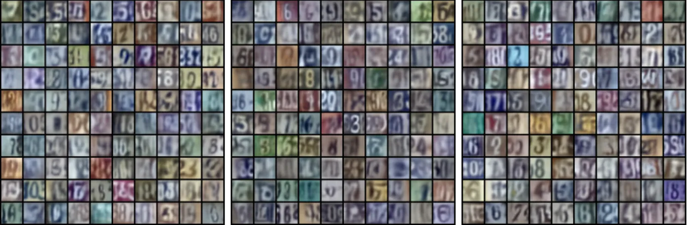
Figure 4.1 shows synthesized samples for each amount of unannotated training data given to the generative model: 40,000, 80,000, and 120,000 examples. These synthesized samples were obtained from the generator network and associated hyperparameters that ultimately produced the best classification accuracy.
Figure 4.1: Synthesized samples using 40,000, 80,000, and 120,000 training examples
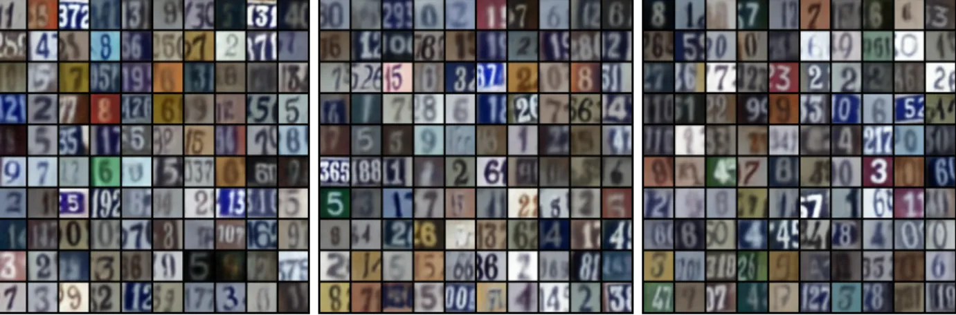
given to the generative model: 40,000, 80,000, and 120,000 examples. An observed image x is reconstructed simply by running gradient descent on the least-squares loss function L(z) = kx−gθ(z)k2. The Langevin dynamics is initialized from z0 ∼ p0(z) and iterates zt+1 = zt− ηtL0(zt). The inferred z and the learned θ weights of the generative model collaborate to reconstruct the observed example x.
Figure 4.2: Reconstructed samples using 40,000, 80,000, and 120,000 training examples
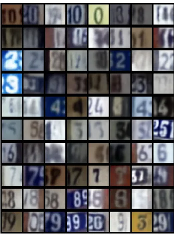
Figure 4.3: Reconstructed samples in which each row represents a digit
4.3
Quantitative Results
The mean-squared error (MSE) of reconstructed samples and the Fr´echet Inception Distance (FID) [46] score of synthesized samples are used to quantitatively evaluate the learning of the generative model.
The MSE is calculated between training examples and their reconstructions. The FID evaluation metric uses the Inception v3 classifier [47]. The FID is a calculation of the distance between the Inception v3 classifier activations for observed and synthesized examples; a lower FID score corresponds to higher-fidelity synthesized samples.
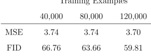
Table 4.1 displays the MSE and FID values obtained for each amount of unannotated training data given to the generative model: 40,000, 80,000, and 120,000 examples.
Training Examples 40,000 80,000 120,000
MSE 3.74 3.74 3.70
FID 66.76 63.66 59.81
Table 4.1: MSE and FID using 40,000, 80,000, and 120,000 training examples
4.4
Classification
During evaluation, the Short Run classifier may generate multiple latent variables {zi, i = 1, . . . , n}for one test examplex, as a means to improve classification accuracy. This form of inference is made reasonable by the stochasticity of the Langevin equation. z is a random variable. With multiplezsampled for onex, it becomes feasible to take advantage of various accuracy methods:
(1) Multiple z may be averaged to then give to the classifier to obtain a prediction ˆy. (2) Multiple z may be given to the classifier to then average over the logits output by the classifier, i.e., the output of the last layer before it is fed to an activation function.
(3) Multiple z may be given to the classifier to then obtain multiple predictions ˆy for which to find the mode, which is the final predicted label.
Table 4.2 displays the classification accuracy of the Short Run classifier given each amount of unannotated training data given to the generative model: 40,000, 80,000, and 120,000 training examples. The ConvNet classifier achieved 86.5% accuracy in comparison. However, the improvements in accuracy given additional unannotated data suggest the accuracy of the Short Run classifier could surpass that of the ConvNet classifier.
Training Examples 40,000 80,000 120,000 Accuracy (%) 79.0 80.0 80.8
Table 4.2: Classification accuracy using 40,000, 80,000, and 120,000 training examples
4.5
Adversarial Robustness
The vulnerability of neural networks to adversarial attacks is a fundamental problem in deep learning today. Neural network sensitivity may be exploited to create adversarial signals that cause trained networks to produce defective results, undermining model robustness. In many cases, only small perturbations, hardly perceptible to a human, are necessary to induce a misclassification.
Szegedy et al. [48] was the first to point out that several machine learning models, includ-ing state-of-the-art neural networks, are vulnerable to adversarial examples. Interestinclud-ingly, models of different architectures or trained on different subsets of training data often all misclassify the same adversarial example [49].
Currently, the most successful defense method is adversarial training, in which a classifier is trained with adversarial examples created during learning. Another approach is adversar-ial purification, in which an input image is purified to remove adversaradversar-ial signals before it is classified. [50] uses MCMC sampling with an EBM for adversarial purification. The mem-oryless behavior of long-run MCMC sampling removes adversarial signals, while metastable behavior preserves consistent appearance of the MCMC samples after many steps, allowing for accurate long-run prediction. It is the first use of an EBM as an effective adversarial defense against white-box attacks, for naturally trained image classifiers [50].
[49] introduces the Fast Gradient Sign Attack, which is a remarkably powerful and yet intuitive adversarial attack. FGSM attacks neural networks by leveraging the way they learn,
i.e., their gradients. Instead of minimizing loss by updating parameters based on backprop-agated gradients, typical of neural networks, FGSM perturbs input data to maximize loss. FGSM is a white-box adversarial attack, in which it is assumed the adversary has full knowl-edge of the classifier, including the architecture, inputs, outputs, weights, and in particular, gradients. White-box attacks are the strongest attacks against the majority of adversarial defenses [50].
Letθbe the parameters of the classifier under attack, in this case the Short Run classifier or the ConvNet classifier. Let x be an observed example, y the associated label for x, and Ldis(θ, x, y) the discriminative loss function used to train the classifier. The loss function may be linearized around the current value ofθ to obtain an optimal, max-norm constrained perturbation of
η=sign( ∂
∂xLdis(θ, x, y)). (4.2)
The FGSM attack backpropagates the gradient back to the input data to calculate ∂
∂xLdis(θ, x, y). Then, it adjusts the input data by a small step in the direction that maximizes loss, i.e., sign∂x∂Ldis(θ, x, y) [49].
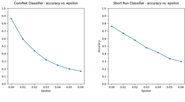
Figure 4.4 shows the effect of the FGSM adversarial attack on the ConvNet and Short Run classifiers. The parameter controls the degree of perturbation added to the images. Increasing the value offurther degrades model accuracy as more perturbation is introduced. With even a small amount of adversarial perturbation added, i.e.,= 0.01, the Short Run classifier (68.4%) already achieves better classification accuracy than the ConvNet classifier (59.5%). At = 0.03, the difference between the Short Run classifier (48.4%) and the ConvNet classifier (30.6%) is nearly 20%.
The Short Run classifier exhibits robustness due to (1) the stochasticity of the Langevin equation, which adds randomness to the process used to form classification prediction ˆy, and (2) the top-down architecture of the generator network, which adds a layer of indirection, i.e. x→z →yˆ, to the process used to form ˆy, in comparison to the ConvNet processx→yˆ.
Figure 4.4: Effect of adversarial attack on ConvNet and Short Run classifiers
Figure 4.5 shows an example of misclassified training examples due to the FGSM adver-sarial perturbations. The first row shows original images with no perturbation. The title of each image has an arrow pointing from the original prediction to the adversarial prediction. Note how the perturbations start to become evident at = 0.4 and are quite evident at = 0.6. However, in almost all cases humans are capable of identifying the correct class for the digit despite the added perturbation, implying that an ideal machine learning model should do the same.
CHAPTER 5
Conclusion
Introduced in this study is a deep generative classifier employing Short Run MCMC infer-ence with Langevin dynamics and backpropagation through time. Based on the alternating backpropagation algorithm, the Short Run classifier performs explicit explain-away inference of latent variables, and without the need for an extra inference network. The top-down ar-chitecture of the generator network allows for data analysis, synthesis, and embedding and helps to counteract the effect of adversarial perturbations. The non-convergent, non-mixing, non-persistent nature of Short Run MCMC lends an efficient inference method for the gen-erator network, with the Langevin dynamics acting as a k-step residual network, or RNN, for which backpropagation through time may occur.
In contrast to a ConvNet classifier with analogous architecture, the Short Run classifier (1) may synthesize data, (2) may learn unsupervised from additional unannotated data, and (3) exhibits robustness to adversarial attacks, due to the stochasticity of the Langevin equation and the top-down architecture of the generator network. The ConvNet classifier lacks the ability to perform (1) or (2) and possesses no defense against adversarial attacks, a critical concern for any deployed machine learning system. Furthermore, improvements in accuracy given additional unannotated data suggest the accuracy of the Short Run classifier could surpass that of the ConvNet classifier.
APPENDIX A
Appendix
A.1
Model Architectures
In the following, nf denotes the number of output feature maps and nf ∈ {64,128}. ConvT(nf) denotes a transposed convolutional operation with nf output feature maps and corresponding bias terms.
Generator
Layers Output Size Stride Padding
Input 200 3 x 3 ConvT(nf2), Mish (nf2 x 3 x 3) 1 0 4 x 4 ConvT(nf2), Mish (nf2 x 7 x 7) 2 1 4 x 4 ConvT(nf1), Mish (nf1 x 14 x 14) 2 1 4 x 4 ConvT(3), Mish (3 x 28 x 28) 2 1 Sigmoid (3 x 28 x 28)
Table A.1: Generator network structure
In the following, Conv(nf) denotes a convolutional operation with nf output feature maps and corresponding bias terms.
Small Classifier
Layers Output Size
Input 200
Linear, Mish 140
Linear, Mish 80
Linear, Mish 10
Table A.2: Small classifier network structure
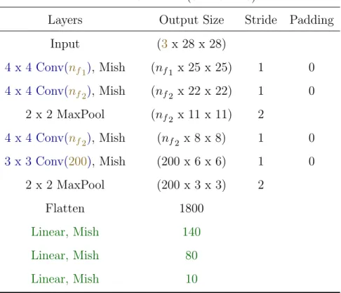
ConvNet Classifier (3 x 28 x 28)
Layers Output Size Stride Padding Input (3 x 28 x 28) 4 x 4 Conv(nf1), Mish (nf1 x 25 x 25) 1 0 4 x 4 Conv(nf2), Mish (nf2 x 22 x 22) 1 0 2 x 2 MaxPool (nf2 x 11 x 11) 2 4 x 4 Conv(nf2), Mish (nf2 x 8 x 8) 1 0 3 x 3 Conv(200), Mish (200 x 6 x 6) 1 0 2 x 2 MaxPool (200 x 3 x 3) 2 Flatten 1800 Linear, Mish 140 Linear, Mish 80 Linear, Mish 10
REFERENCES
[1] Alex Krizhevsky, Ilya Sutskever, and Geoffrey E Hinton. Imagenet classification with deep convolutional neural networks. In F. Pereira, C. J. C. Burges, L. Bottou, and K. Q. Weinberger, editors, Advances in Neural Information Processing Systems 25, pages 1097–1105. Curran Associates, Inc., 2012.
[2] Yoshua Bengio, Yann Lecun, and Yann Lecun. Convolutional networks for images, speech, and time-series, 1995.
[3] Song Zhu, Yingnian Wu, and David Mumford. Filter, random field and maximum entropy. Neural Computation - NECO, 01 1997.
[4] Mitch Hill, Erik Nijkamp, and Song-Chun Zhu. Building a telescope to look into high-dimensional image spaces, 2018.
[5] Ruslan Salakhutdinov and Geoffrey Hinton. Deep boltzmann machines. In David van Dyk and Max Welling, editors, Proceedings of the Twelth International Conference on Artificial Intelligence and Statistics, volume 5 of Proceedings of Machine Learning Re-search, pages 448–455, Hilton Clearwater Beach Resort, Clearwater Beach, Florida USA, 16–18 Apr 2009. PMLR.
[6] Ruiqi Gao, Yang Lu, Junpei Zhou, Song-Chun Zhu, and Ying Nian Wu. Learning generative convnets via multi-grid modeling and sampling, 2017.
[7] Ruiqi Gao, Erik Nijkamp, Diederik P. Kingma, Zhen Xu, Andrew M. Dai, and Ying Nian Wu. Flow contrastive estimation of energy-based models, 2019.
[8] Jianwen Xie, Ruiqi Gao, Erik Nijkamp, Song-Chun Zhu, and Ying Nian Wu. Represen-tation learning: A statistical perspective, 2019.
[9] Junbo Zhao, Michael Mathieu, and Yann LeCun. Energy-based generative adversarial network, 2016.
[10] Tian Han, Erik Nijkamp, Xiaolin Fang, Mitch Hill, Song-Chun Zhu, and Ying Nian Wu. Divergence triangle for joint training of generator model, energy-based model, and inference model, 2018.
[11] Tian Han, Yang Lu, Song-Chun Zhu, and Ying Nian Wu. Alternating back-propagation for generator network, 2016.
[12] Ying Nian Wu, Ruiqi Gao, Tian Han, and Song-Chun Zhu. A tale of three probabilistic families: Discriminative, descriptive and generative models, 2018.
[13] Ian Goodfellow, Jean Pouget-Abadie, Mehdi Mirza, Bing Xu, David Warde-Farley, Sherjil Ozair, Aaron Courville, and Yoshua Bengio. Generative adversarial nets. In Z. Ghahramani, M. Welling, C. Cortes, N. D. Lawrence, and K. Q. Weinberger, edi-tors, Advances in Neural Information Processing Systems 27, pages 2672–2680. Curran Associates, Inc., 2014.
[14] Diederik P Kingma and Max Welling. Auto-encoding variational bayes, 2013.
[15] Donald B. Rubin and Dorothy T. Thayer. Em algorithms for ml factor analysis. Psy-chometrika, 47(1), March 1982.
[16] A. P. Dempster, N. M. Laird, and D. B. Rubin. Maximum likelihood from incomplete data via the em algorithm. Journal of the Royal Statistical Society. Series B (Method-ological), 39(1):1–38, 1977.
[17] Don Lemons and Anthony Gythiel. Paul langevin’s 1908 paper “on the theory of brow-nian motion”. American Journal of Physics - AMER J PHYS, 65:1079–1081, 01 1997. [18] Adrian Barbu and Song-Chun Zhu. Monte Carlo Methods. Springer, 2020.
[19] Yizhou Wang and Zhu. Modeling textured motion : particle, wave and sketch. In
Proceedings Ninth IEEE International Conference on Computer Vision, pages 213–220 vol.1, 2003.
[20] Jianwen Xie, Ruiqi Gao, Zilong Zheng, Song-Chun Zhu, and Ying Nian Wu. Learning dynamic generator model by alternating back-propagation through time, 2018.
[21] S. Geman and D. Geman. Stochastic relaxation, gibbs distributions, and the bayesian restoration of images. IEEE Transactions on Pattern Analysis and Machine Intelli-gence, PAMI-6(6):721–741, 1984.
[22] Radford M. Neal. Mcmc using hamiltonian dynamics, 2012.
[23] Erik Nijkamp, Mitch Hill, Song-Chun Zhu, and Ying Nian Wu. Learning non-convergent non-persistent short-run mcmc toward energy-based model, 2019.
[24] Erik Nijkamp, Mitch Hill, Tian Han, Song-Chun Zhu, and Ying Nian Wu. On the anatomy of mcmc-based maximum likelihood learning of energy-based models, 2019. [25] Erik Nijkamp, Bo Pang, Tian Han, Linqi Zhou, Song-Chun Zhu, and Ying Nian Wu.
Learning deep generative models with short run inference dynamics, 2019.
[26] Ulf Grenander and Michael Miller. Pattern Theory: From Representation to Inference. Oxford University Press, Inc., USA, 2007.
[27] Jianwen Xie, Yang Lu, Song-Chun Zhu, and Ying Nian Wu. A theory of generative convnet, 2016.
[28] Long Jin, Justin Lazarow, and Zhuowen Tu. Introspective classification with convolu-tional nets, 2017.
[29] M. Carreira-Perpinan and G. Hinton. On contrastive divergence learning. 01 2005. [30] Tijmen Tieleman. Training restricted boltzmann machines using approximations to the
likelihood gradient. pages 1064–1071, 01 2008.
[31] Jiquan Ngiam, Zhenghao Chen, Pang Wei Koh, and Andrew Y. Ng. Learning deep energy models. In ICML, pages 1105–1112, 2011.
[32] Dandan Zhu, Tian Han, Linqi Zhou, Xiaokang Yang, and Ying Nian Wu. Deep unsu-pervised clustering with clustered generator model, 2019.
[33] Ian Goodfellow, Yoshua Bengio, and Aaron Courville. Deep Learning. MIT Press, 2016.
http://www.deeplearningbook.org.
[34] Herbert Robbins and Sutton Monro. A stochastic approximation method. The Annals of Mathematical Statistics, 22(3):400–407, 1951.
[35] P. J. Werbos. Backpropagation through time: what it does and how to do it. Proceedings of the IEEE, 78(10):1550–1560, 1990.
[36] Timothy Lillicrap and Adam Santoro. Backpropagation through time and the brain.
Current Opinion in Neurobiology, 55:82–89, 04 2019.
[37] Less Wright. Ranger deep learning optimizer. https://github.com/lessw2020/ Ranger-Deep-Learning-Optimizer, 2019.
[38] Diganta Misra. Mish: A self regularized non-monotonic neural activation function, 2019.
[39] Liyuan Liu, Haoming Jiang, Pengcheng He, Weizhu Chen, Xiaodong Liu, Jianfeng Gao, and Jiawei Han. On the variance of the adaptive learning rate and beyond, 2019. [40] Michael R. Zhang, James Lucas, Geoffrey Hinton, and Jimmy Ba. Lookahead optimizer:
k steps forward, 1 step back, 2019.
[41] Hongwei Yong, Jianqiang Huang, Xiansheng Hua, and Lei Zhang. Gradient centraliza-tion: A new optimization technique for deep neural networks, 2020.
[42] Yurii Nesterov. Lectures on Convex Optimization. Springer Publishing Company, In-corporated, 2nd edition, 2018.
[43] Amir Beck. First-Order Methods in Optimization. Society for Industrial and Applied Mathematics, Philadelphia, PA, 2017.
[44] Yuval Netzer, Tao Wang, Adam Coates, Alessandro Bissacco, Bo Wu, and Andrew Ng. Reading digits in natural images with unsupervised feature learning. NIPS, 01 2011. [45] Yann Lecun, L´eon Bottou, Yoshua Bengio, and Patrick Haffner. Gradient-based learning
applied to document recognition. InProceedings of the IEEE, pages 2278–2324, 1998. [46] Martin Heusel, Hubert Ramsauer, Thomas Unterthiner, Bernhard Nessler, and Sepp
Hochreiter. Gans trained by a two time-scale update rule converge to a local nash equilibrium, 2017.
[47] Christian Szegedy, Vincent Vanhoucke, Sergey Ioffe, Jon Shlens, and ZB Wojna. Re-thinking the inception architecture for computer vision. 06 2016.
[48] Christian Szegedy, Wojciech Zaremba, Ilya Sutskever, Joan Bruna, Dumitru Erhan, Ian Goodfellow, and Rob Fergus. Intriguing properties of neural networks, 2013.
[49] Ian J. Goodfellow, Jonathon Shlens, and Christian Szegedy. Explaining and harnessing adversarial examples, 2014.
[50] Mitch Hill, Jonathan Mitchell, and Song-Chun Zhu. Stochastic security: Adversarial defense using long-run dynamics of energy-based models, 2020.