Forecasting mortgage securitization risk under systemic risk and parameter uncertainty

(1)

Research Working Paper Series

Forecasting Mortgage Securitization Risk under Systemic

Risk and Parameter Uncertainty

Professor Dr Daniel Rosch

Department of Statistics

Faculty of Business, Economics and Business Information Systems

University of Regensburg, Germany

Associate Professor Harald Scheule

Finance Discipline Group

UTS Business School

University of Technology, Sydney

WORKING PAPER NO. 009/2014 MARCH 2014

www.cifr.edu.au

This research was supported by the Centre for International Finance and Regulation (project number E001) which is funded

(2)

The contents of this paper reflect the views of the author and do not represent the official views or policies of the Centre for International Finance and Regulation or any of their Consortium members. Information may be incomplete and may not be relied upon without seeking prior professional advice. The Centre for International Finance and Regulation and the Consortium partners exclude all liability arising directly or indirectly from use or reliance on the information contained in this publication.

(3)

Forecasting Mortgage Securitization Risk

under Systematic Risk and Parameter

Uncertainty

Daniel R¨

osch

a

Harald Scheule

b

a_{Department of Statistics, Faculty of Business, Economics and Business}

Information Systems, University of Regensburg, 93040 Regensburg, Germany, Phone: +49-941-943-2570, Fax : +49-941-943-4936,

mailto:[email protected]

b_{Finance Discipline Group, UTS Business School, University of Technology,}

Sydney, PO Box 123, Broadway NSW 2007, Australia, Phone: +61-2-9514-7724, Fax: +61-2-9514-7722, mailto: [email protected]

(4)

Forecasting Mortgage Securitization Risk

under Systematic Risk and Parameter

Uncertainty

Abstract

The Global Financial Crisis exposed financial institutions to severe unexpected

losses in relation to mortgage securitizations and derivatives. This paper finds that

risk models such as ratings are exposed to a large degree of systematic risk and

parameter uncertainty. An out-of-sample forecasting exercise of the financial crisis

shows that a simple approach addressing both issues is able to produce ranges for

risk measures consistent with realized losses. This explains how financial markets

were taken by surprise in relation to realized losses.

JEL classification:G20; G28; C51

Keywords: Economic Capital; Global Financial Crisis; Home Equity Loan

Security; Mortgage-backed Security; Parameter Uncertainty; Rating;

(5)

1 Introduction

Securitization ratings applied by credit rating agencies (CRAs) were identified as a source of the Global Financial Crisis (GFC) (compare Hull, 2009). Financial markets, which rely on credit ratings were surprised by the high levels of impairment rates and large number of downgrades of seemingly high quality (e.g., AAA-rated) mortgage-backed securities from 2007 to 2009.

Table 1 supports this point by comparing the impairment rates for Baa-rated mortgage-backed securities (MBSs) with Baa-rated home equity loan securities (HELs). Both MBSs and HELs are securitizations of real-estate collateralized loan portfolios.1 Impairment rates for MBSs and HELs were well below 10 basis points before the GFC and peaked at 20.7% (MBSs) and 28.2% (HELs), respectively, during the GFC.

[insert Table 1 here]

Investors relied on CRA ratings and expected impairment rates similar to the historic expe-rience for such ratings. Credit ratings reflect expectations about future impairment risk.

Our paper has two main objectives. Firstly, we theoretically and empirically analyze the magnitudes of deviations of realized impairments of securitizations from their expectations implied by credit ratings, that is, the exposure of securitizations to systematic risk. Sec-ondly, we show that measuring systematic risk with an econometric model is subject to a large amount of parameter uncertainty. These two issues are highly related as histories of credit data are generally limited in relation to the time-series, which leads to an increase in parameter uncertainty as well as underestimation of systematic risk if the empirical experi-ence is limited to periods of economic expansion. Our study shows that this was the case for

1 _{MBSs are collateralized by prime mortgages and HEL securities are mostly collateralized by}

(6)

mortgage securitization prior to the GFC.

This paper’s research question is most closely related to the following literature: Heitfield (2010) who argues that credit ratings do not include information on systematic risk and uncertainty and Coval et al. (2009) who show that variations of the pool default correlation may have a substantial impact on the risk of the tranches. Time series information for parameter estimation is limited for securitization data due to the recent origination of these financial instruments and parameter uncertainty is thus particularly pronounced for time-varying explanatory variables. With regard to systematic risk, Loeffler (2004) finds that the power of ratings to predict default for corporate bonds is low due to the ‘though-the-cycle’ nature of CRA rating systems, which implies that CRAs aim to rate by considering borrower-specific information and not macroeconomic information. Parameter instability and uncertainty has been addressed by Jorion (1996) and Escanciano and Olmo (2010) for market risk and more recently by Tarashev and Zhu (2008) for credit risk.

This paper’s technical framework is based on work by Heitfield (2009) who shows the impact of estimation errors in pool correlations on the risk measures and ratings of tranches in a sim-ulation study. This paper extends Heitfield (2010) by introducing a pool-specific risk factor following Gordy and Howells (2006), Pykhtin and Dev (2002) and Gordy and Jones (2003) to reflect correlation between loans in a portfolio underlying a securitization.2 _{In extension}

to previous literature our paper provides an empirical parameter estimation approach for these models and applies it to a comprehensive dataset of securitizations.

The paper is also related to several other streams in the literature. One stream measures the inherent actuarial credit risk (also known as physical risk) of the asset portfolio underlying a securitization transaction. The main aim in this field of research is to develop approaches for modeling and forecasting the distribution of future credit losses based on individual risk

2 _{Related literature looks at market prices of credit derivatives and develops risk-neutral pricing}

models. Credit derivatives are structurally similar to securitizations. Prominent approaches are due to Li (2000), Hull and White (2004) and Longstaff and Rajan (2008).

(7)

parameters, such as the default probability. The parameters are aggregated to a portfolio risk distribution. Important approaches which address the default probability are due to Merton (1974), Leland (1994), Jarrow and Turnbull (1995), Longstaff and Schwartz (1995), Madan and Unal (1995), Leland and Toft (1996), Jarrow et al. (1997), Duffie and Singleton (1999), Shumway (2001), Carey and Hrycay (2001), Crouhy et al. (2001), Koopman et al. (2005), McNeil and Wendin (2007) and Duffie et al. (2007). In addition, Dietsch and Petey (2004) and McNeil and Wendin (2007) model the correlations between default events. Carey (1998), Acharya et al. (2007), Pan and Singleton (2008), Qi and Yang (2009), Grunert and Weber (2009) and Bruche and Gonz´alez-Aguado (2010) develop economically motivated empirical models for recoveries using explanatory co-variables. Altman et al. (2005) model correlations between default events and loss rates given default.

A second stream of literature deals with rating issues before and during the GFC. Benmelech and Dlugosz (2009) show empirically that rating inflation was an issue in the GFC and they argue that one of the causes of the crisis was overconfidence in statistical models. The authors use rating migration statistics and analyze up- and downgrades during the crisis. Ashcraft et al. (2010) find that CRA ratings for mortgage-backed securities provide useful information for investors, show significant time variation and become less conservative prior to the GFC. Griffin and Tang (2012) compare CRA model methodologies with CRA ratings for collateralized debt obligations and find that rating models are more accurate than the actual ratings. Black et al. (2011) find considerable differences in loan performance across originator types of Commercial Mortgage Backed Securities (CMBS) after controlling for credit characteristics, which suggests presence of moral hazard. R¨osch and Scheule (2012) compare capital adequacy regulations with risk characteristics of securitizations and find capital arbitrage opportunities. L¨utzenkirchen et al. (2013) analyze whether current ratings-based rules for regulatory capital of securitizations reflect the exposure to systematic risk. Harrington (2009) analyzes the causes of the GFC and the consequences on the US insurer AIG.

(8)

The main contribution of this paper is to provide an empirical analysis of systematic risk and parameter uncertainty for securitizations with data before and during the financial crisis. The paper shows the magnitude of systematic risk exposure and parameter uncertainty. An out-of-sample forecasting analysis of the financial crisis shows that a simple approach addressing both issues may have been able to anticipate the magnitude of losses realized during the GFC. Systematic risk and parameter uncertainty may not have been included in impairment risk measures prior to the GFC. If they had been, the high impairment rates would not have been as ‘surprising’ as the observation of the reactions of financial markets, institutions and instruments suggested.

Please note that the present paper does not address the time-series correlation of systematic risk. We have chosen to follow this path as (i) credit ratings change very infrequently (in the 13 years of observations only 6.6% of MBS ratings (10.5% of HEL ratings) are downgraded and only 1.5% are upgraded (0.7% of HEL ratings) and (ii) investors often rely on these credit ratings to make investment decisions. The paper analyzes the additional portfolio risk (measured by value-at-risk) under this approach. Duffie, Eckner, Horel and Saita (2009) and Koopman et al. (2011) have shown that systematic risk is serially correlated. In the future, credit rating methodologies may change to include such an approach.

The paper progresses as follows: Section 2 provides the model framework based on the ex-isting literature. Section 3 describes the data, estimates ratings-based models and analyzes out-of-sample point and distribution forecasts for the value-at-risk (VaR). Section 4 summa-rizes the findings.

2 Model Framework

This paper’s technical framework is based on work by Heitfield (2009) who shows the impact of estimation errors in pool correlations on the risk measures and ratings of tranches in a

(9)

simulation study. For modeling the asset pool risk and the impairment risk of securitized tranches, this paper follows Vasicek (1987, 1991); Gordy (2000, 2003) and Li (2000) who develop a latent factor credit risk model, which is consistent with Merton (1974). The model assumes that a single borrower k exhibits a credit default in time period t if the return Rkt

on his assets crosses some threshold ct (k = 1, ..., K;t = 1, ..., T). In the Gaussian model

variant the asset return is assumed to be normally distributed.3 LetRkt be standardized to

have mean of zero and standard deviation of one and be driven by a common time-specific systematic risk factor Xt and an idiosyncratic (i.e., diversifiable) factor Ukt, both being

standard normally distributed and independent from each other, with standardized weights

ρt and √ 1−ρt, that is Rkt= √ ρtXt+ q 1−ρtUkt (1)

If many borrowers are pooled the default ratePt of the pool which measures the ratio of the

number of defaulting borrowers and the total number of borrowers within the pool converges in probability against the conditional default probability (see e.g., Kupiec, 2009):

Pt= PK k=11{Rkt<ct} K p → Φ ct− √ ρtXt √ 1−ρt ! asK → ∞ (2)

where 1{Rkt<ct} is an indicator variable which equals one if Rkt < ct and zero otherwise.

The right hand side of Equation (2) is the asymptotic default rate of a pool. Introducing the subscript i for a pool (or deal), the asymptotic default rate of pool i in time period t

(i= 1, ..., I;t= 1, ..., T) is then modeled as

3 _{Please note that a non-linear transformation ensures that distributions of risk measures such as}

probability of default, default rate or loss rate are highly skewed. In other words the propensity of large losses is higher than a normal distribution would suggest.

(10)

Pit = Φ cit− √ ρitXit √ 1−ρit ! (3)

whereXit is a time-specific systematic risk factor which affects all assets in the pool jointly.

√

ρit is the exposure of the asset returns in the pool to this factor. cit = Φ−1(πit) is the

default threshold, where πit is the probability of default (PD) and Φ−1(·) is the inverse of

the standard normal CDF.

The CDFF(·) of the default rate Pit in pooli are then given by

F(pit) = Φ √ 1−ρitΦ−1(pit)−Φ−1(πit) √ ρit ! (4)

Impairment of a tranchej occurs if the pool default rate is higher than the attachment level

ALijt of the tranche, i.e., Pit > ALijt. The tranche impairment probability is then given as

P({Pit > ALijt}) = 1−Φ √ 1−ρitΦ−1(ALijt)−Φ−1(πit) √ ρit ! = Φ Φ −1₍_π it)− √ 1−ρitΦ−1(ALijt) √ ρit ! = Φ (ηijt) (5)

Following Gordy and Howells (2006) and Pykhtin and Dev (2002), this paper introduces an economy-wide ‘super’-factor which affects all pools in the economy jointly to reflect cor-relation between pools of securitizations. Therefore, the pool-specific factor is decomposed into

(11)

Xit=

q

δit·Xt∗+

q

1−δit·Uit (6)

where X_t∗ is a univariate standard normally distributed ‘super’-factor measuring the state of the economy. Uit is a standard normally distributed pool-specific factor. δit measures the

strength of dependence across pools. This paper assumes δit = δ for all pools for efficiency.

The conditional tranche impairment probability can thus be stated as a function of the systematic factor by P({Pit> ALijt}|Xt∗) = Φ Φ−1₍_π it)− √ 1−ρitΦ−1(ALijt)− √ ρit √ δX_t∗ √ ρit √ 1−δ ! = Φηijt/ √ 1−δ+b·X_t∗ (7)

where b=−√δ/√1−δ is the transformed exposure to the ‘super-factor’. The expressionηijt/

√

1−δ may be modeled by observable tranche characteristics such that

ηijt/

√

1−δ=β0xijt, wherexijtare observable variables and βis a vector of parameters. The

model can then be stated in terms of a mixed effects probit regression with fixed effects xijt

and random effects X_t∗ or ‘frailty’ model (see Duffie, Eckner, Horel and Saita, 2009) as

P ({Pit> ALijt}|Xt∗) = Φ (β

0

xijt+b·Xt∗) (8)

In the empirical analysis xijt will be the intercept per rating and securitization category.

It is obvious that the higher the degree to which tranches are exposed to the common economy-wide factor, the higher the dispersion (here standard deviation)b is and the higher the expected deviations of the realized tranche impairment probability from the expected probability of Equation (5) are.

(12)

The dispersion parameter b of the random effect model can be interpreted after reparame-terization in a similar fashion as an ‘asset correlation’:

P ({Pit > ALijt}|Xt∗) = Φ e β0xijt+ √ δ·X_t∗ √ 1−δ ! (9) where δ= ₁₊b2_b2 and βe=β· √ 1−δ.

The probability of observing a pattern of tranche impairments in period t, conditional on the super-factor x∗_t in Equation (8) is then

ϕ(x∗_t) =P(1{P1t>AL1jt}, ...,1{PIt>ALIjt}|x

∗ t) = I Y i=1 Φ (β0xijt+b·x∗t) 1{_Pit>ALijt} (1−Φ (β0xijt+b·x∗t)) 1−1{_Pit>ALijt} (10)

wherej is the tranche with the given credit rating in the respective pool. This results in the likelihood L= Z · · · Z T Y t=1 ϕ(x∗_t)f(x∗₁)· · ·f(x∗_T) dx∗₁dx∗_T (11)

The estimators exist asymptotically, are consistent and converge to normality, (see Davidson and MacKinnon, 1993). The consistency of parameter estimates were confirmed in a Monte-Carlo simulation study.

(13)

3 Empirical Analysis

3.1 The Data

The paper analyzes a unique and extensive panel data set of US mortgage securitization (MBSs and HELs) during the years 1997 to 2009.4 _{The data contains 281,035 annual}

ob-servations for MBSs (177,493) and HELs (103,542) securitizations and 19,291 impairment events (MBSs: 9,277, HELs: 10,014). Loss events are traditionally called impairment events for securitizations and cover principal and interest payment shortfalls as well as downgrades to Ca/C.

The data covers Moody’s credit ratings for the tranches. Please note that the only information this paper uses, which is uniquely generated by Moody’s, is the credit rating. Moody’s credit ratings are very similar to the ones published by other rating agencies such as Standard & Poor’s and Fitch: we have hand-collected from the Bloomberg database ratings at origination for Fitch, Moody’s and Standard & Poor’s. The Spearman correlation coefficient is in excess of 97% for all pairwise combinations of rating agencies. This analysis suggests that credit ratings are similar for the three rating agencies as the correlation coefficients are very high and is consistent with interviews with financial analysts of the three CRAs as well as the literature in relation to bond ratings.5

Table 1 shows the number of observations and impairment rate per rating category for mortgage-backed securities (Panel A) and home equity loan securitizations (Panel B). HELs include to a large extent sub-prime mortgage loans. The number of observed tranches in-creases over time, which reflects the growth of these financial instruments over recent years.

4 _{Securitizations have also become important for managing insurable risks, see Cummins and}

Trainar (2009), and Chen and Cox (2009) for mortality securitizations in particular. As US mort-gage securitizations have been made responsible for the GFC, we focus on these classes only.

(14)

The impairment rate increases during the GFC (2008 and 2009) and more generally from rating grades Aaa-A (Aaa, Aa and A) to Baa to Ba to B to Caa.6

3.2 Empirical Models for Systematic Risk

Table 2 shows the estimation results of the mixed effects probit models for MBS and HEL securitizations divided by rating grade for the following sample periods:

• All: whole sample period 1997-2009;

• Pre-2009: restricted sample period 1997-2008;

• Pre-2006: restricted sample period 1997-2005.

We analyze two types of models: one efficient but simple model which aggregates over all securitizations (i.e., Model 1), and one model which controls for credit ratings (i.e., Model 2).7 We proceed with Model 2 as the model allows a joint estimation of rating-implied impairment probabilities and the dispersion parameter. Model 2 may be slightly less efficient than Model 1 and standard errors for the dispersion parameter are comparable for the two models. The different time periods with data before and during the financial crisis are analyzed in order to (i) check how the parameter estimates change due to the high number of impairments during the crisis, and (ii) to conduct an out-of-sample forecasting exercise where we use data up to yeart (i.e., before the crisis) for parameter estimation and forecast risk figures for year t+ 1 (i.e., the crisis).

[Table 2 about here.]

6 _{Note that the impairment rate for all data is calculated as the average of the annual impairment}

rate.

(15)

The coefficients for the ratings (i.e., the intercepts) increase with a decrease in rating qual-ity.8 This is in line with our expectation as well as the descriptive analysis as a lower credit quality, which is indicated by the credit rating, should imply a higher impairment probability. The coefficients for the unobservable systematic effect are statistically significantly different from zero in most models. This shows that there is a significant systematic effect, which leads to deviations of the impairment rate realizations from their expectations. Moreover, the estimates for b for the whole sample period are larger than for the pre-crisis periods (until 2009 and pre-2008). This suggests that the data from the crisis adds new information and, thus, the crisis might have been difficult to forecast with data before the crisis. The exposure of the systematic factor varies between MBS and HEL. Note that the estimated standard errors are high for the systematic risk exposures. This reflects the high degree of parameter estimation uncertainty, which is due to the relatively short time series. Note also that the standard errors increase from 1997-2005 to 1997-2009 due to the GFC despite a slightly longer time series.

The paper differentiates between MBS (prime mortgage portfolio) and HEL (sub-prime mortgage portfolio) secutitizations. The concern may be raised that the chosen data sets are heterogeneous in nature. In particular, HEL securitizations may include a wider range of securities backed by subprime mortgage loans, home improvement loans, high loan to value loans, home equity lines of credit, and closed-end second-lien loans, as well as net interest margin securitizations (compare Moody’s Investors Service, 2009). In other words, the parameter estimates may differ for subsets of the portfolio. In order to test the im-pact of sub-samples on the parameter estimates, Model (2) (all data) from Table 2 (MBS)

8 _{For MBS, in the models pre-2007 and pre-2006 the coefficient for grade Caa-C could not be}

estimated due to a small number of observations in that grade and the estimate for b resulted in the corner solution of zero.

(16)

and Table 3 (HEL) was scrutinized by a bootstrap analysis.9 _{Random samples of 50% of}

the data were drawn in 200 iterations and summarized by the moments of their empirical distributions in Table 4. Note that the presented models involve computational intensive estimation processes. Panel A reports the results for MBS securitizations and Panel B for HEL securitizations.

The results suggest that the empirical estimates for the complete data set lie well in between the upper and lower moments (i.e., minimum, 25th percentile, 75th percentile and maximum) of the distribution resulting from the bootstrap analysis. This suggests that the sample does not include larger heterogeneous groups. In future extensions, the risk characteristics of such heterogeneous groups could be extended to accommodate information on the loan portfolios, structure and the economy, which ratings do not capture.10 _{Examples for loan variables}

are FICO score, debt to income ratio, loan-to-value ratio, documentation type, mortgage type, property type, or lien position. Examples for structure variables are attachment level, tranche thickness or credit enhancement. Examples for the economic variables are interest rates, unemployment rate or house prices.

3.3 Predictions Using Point Estimates for the Parameters

The model enables the out-of-time prediction of the impairment probability associated with each rating grade after the parameter estimatesbb for the systematic risk exposure and βb for

the intercept of the rating grade are obtained.

The realization of the systematic risk factor is unknown ex ante and we arrive at a distribution

9 _{We thank an anonymous referee for suggesting this analysis.}

10_{Please note that this is the focus of a vibrant literature and references can be found in Section}

(17)

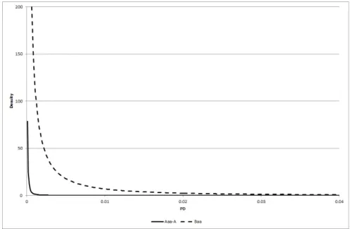
of potential impairment rates, given the point estimates for the parameters. For instance, given the parameter estimates of Model 2 (MBS, pre-2009, see Table 2), the impairment rate densities for the various rating grades of MBS securitizations in 2009 are shown in Figure 1 and Figure 2. The figure shows that a considerable dispersion is introduced by the exposure to the systematic risk factor.

[Figure 1 about here.]

The predicted distribution function is given by

b

F(pijt) =Pb(P_ijt< p_ijt) = Φ    q 1−δbΦ−1(p_ijt)−βbe 0 xijt q b δ    (12)

where _βb_e _and _δ_b_{are given as in Equation (9). The} _α_{-percentile can be calculated as}

b qα = Φ    b_e β 0 xijt+ q b δΦ−1(α) q 1−δb    (13)

Theα-percentile can be interpreted as the value-at-risk. For Model 2 (pre-2006 to pre-2009), the realized pool impairment rate in the subsequent year (i.e., out-of sample) under the respective model is analyzed. For example, the parameters of the models using data up to 2005 (pre-2006) are estimated and a value-at-risk forecast is calculated by Equation (13) and can ex-post be compared with the subsequent impairment realization. This paper proceeds analogously for the other models. This methodology provides an assessment of how well the model performs out-of-sample using rating data prior to the GFC.

(18)

In other words, we look at an investor who (i) analyzes the impairment rates of HELs and MBSs given the information up to a certain period respectively and (ii) calculates the distribution of the potential future impairment rates using historical information based on the point estimates of the parameters. Such an investor acknowledges that systematic risk is present after assessing the risk given credit ratings. This may affect the asset pool tranches via systematic factor realizations. In order to assess extreme events in case of unexpected shocks, the investor calculates an extreme percentile of the distribution (i.e., the value-at-risk) according to Equation (13). A confidence level of 99.97% is exemplarily used.11

The realized impairment rate exceeds the VaR in 2007 and 2008 for most rating grades. The value-at-risk levels are increasing over time as the impairment rates increase. As a result, in 2009, the value-at-risk levels have reached levels which exceed the realized impairment rates. This implies that leveraged investors12 applying the prediction model to determine the minimum capital via the value-at-risk did not have a sufficient level of capital to cover future losses in 2007 and 2008. Taking systematic risk into account is therefore a first and important step in predicting distributions for future impairments or risk figures derived thereof, such as a value-at-risk. However, the challenge is that the accurate estimation of the data generating systematic risk exposure requires a large number of representative realizations.

3.4 Parameter Uncertainty

In the previous subsection the paper uses the Maximum-Likelihoodpoint estimates for fore-casting. However, Table 2 and 3 show that the standard errors for the estimates are

substan-11_{This level is based on industry practice. For example, Deutsche Bank uses 99.98% (compare also}

Hull, 2010, who offers a confidence level of 99.97% as a reference value which banks often use for internal economic capital calculations).

(19)

tial. This is particularly true for the random effect parameter. For example, for Model 2 (all data) and MBS securitizations, the coefficient estimate is 1.1297 and its standard deviation estimate is 0.2368 which is approximately 21% of the coefficient estimate. This implies that an investor who estimates coefficients (e.g., with regard to the systematic exposure) for a securitized tranche, can not be certain that the estimate of the coefficient is correct. This problem is particularly pronounced for short time series (see e.g., Gordy and Heitfield, 2010).

In the following, the impairment probability density associated with each rating grade is predicted taking parameter uncertainty into account. Estimation errors have been addressed in the area of credit risk by Loeffler (2003), Hamerle and R¨osch (2005), Tarashev and Zhu (2008) and Heitfield (2009) by Monte-Carlo simulation studies in a similar manner to Jorion (1996). This paper follows these approaches and simulates distributions for the value-at-risk based on the risk model as well as parameter uncertainty.

The estimated covariance of the parameter estimates is defined as

d

Covψb

=Σb (14)

where ψb is the vector containing all parameter estimates. We randomly draw sample

real-izations for the parameter estimates using this covariance matrix according to

b_b

ψ =ψb+Σb00.5· (15)

is a standard normally distributed random variable, andΣb0.5is the Cholesky Decomposition

such that Σb00.5·Σb0.5 =Σ.b

(20)

is calculated given each sample of random realizations for the parameter estimates according to b_b q_α = Φ     b b_e β 0 xijt+ q b_b δΦ−1₍_α₎ q 1−b_δ_b     (16)

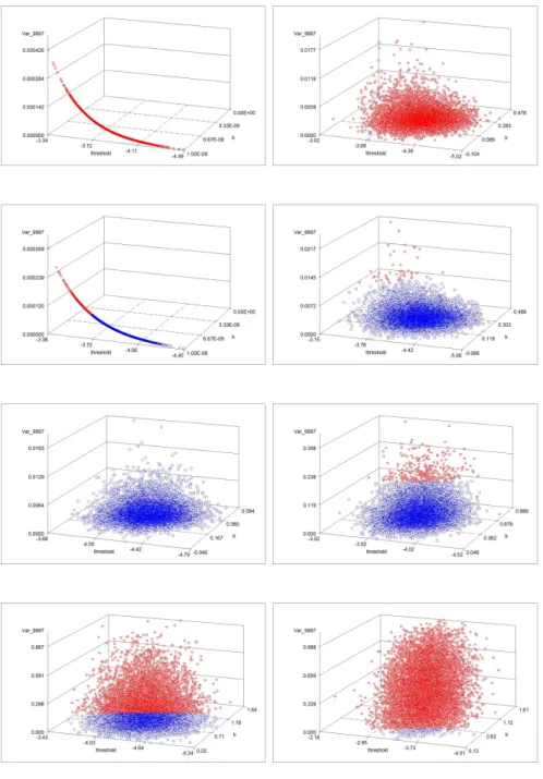
10,000 random iterations are drawn for each rating grade and asset pool which results in a distribution of the 99.97%-economic capital for HELs and MBSs under parameter uncertainty for each rating grade. Figure 3 shows the VaRs (z-axis) for each of the 10,000 randomly simulated settings for the two parameters (intercept on the x-axis, and b on the y-axis) for the years 2006 to 2009 respectively.

Note that the figure focuses on the Aaa-A rating class as this class is most important in terms of securitization volume and counts. The figure shows that the empirical parameter uncer-tainty of the economic capital is very high. The result holds for all analyzed risk segments and asset pool types. The red (blue) dots in the figures show the simulated VaRs which are higher (lower) than the subsequent impairment rate and thus indicate those simulated VaRs which would have (not) covered the realized losses.13

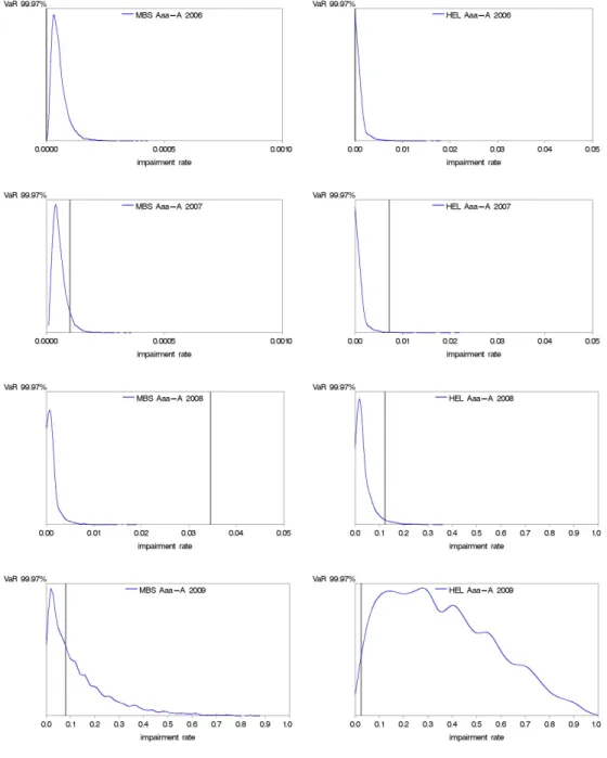
Figure 4 summarizes the economic capital scatters in frequency distributions of the value-at-risk for the Aaa-A rating class. Note that the distribution would collapse to a single point if parameter uncertainty were omitted as in the previous section. The vertical grey lines show the actual impairment rates in that segment in the respective year. As can be seen from

13_{Note that the estimate for the dispersion parameter converged to the corner solution of zero}

for MBS in pre-2006 and pre-2007. Thus, parameter uncertainty is introduced only due to the parameter estimate for the rating coefficient.

(21)

these charts, many of the simulated VaRs are much higher than the ones calculated using point estimates.

These results are confirmed by Table 6 where the VaR derived from point estimates is compared to the 90th and 99th percentiles of the distribution of the VaRs under uncertainty. For example, the 90th percentile of the VaR distribution under uncertainty for Aaa-A rated MBS for 2008 is 0.24% compared to 0.08% which is 3.17 times as high. This ratio can be interpreted as a multiplier or potential add-on factor for VaR due to uncertainty. If the 99th percentile of the VaR distribution is used, the VaR would be 0.60%, which equals a multiplier or add-on factor for VaR of 7.93. This multiplier is different for different ratings and years (due to the different parameter uncertainty) and always greater than or equal to one. It is evident that the largest multipliers are in the Aaa-A rating class, which comprises 82% of all observations. Interestingly, investors were most surprised by the magnitude of losses during the GFC in this low risk class.

Using these extreme VaRs under uncertainty therefore leads to risk figures which are either not exceeded by the realized losses or are exceeded by much less than VaRs which ignore parameter uncertainty. This paper therefore advocates that VaRs should be calculated under parameter uncertainty taking adverse scenarios for the parameters into account which may be very different to measures based on point estimates. Such adverse VaRs dominate in ex-plaining realized losses. Financial market participants, who had been aware of the high degree of systematic risk and parameter uncertaintybefore the financial crisis, would have therefore calculated VaRs, which would have better covered the ‘surprisingly’ high impairment rates of securitizations and implied losses.

(22)

4 Summary

We identify and empirically assess two related issues associated with the measurement of risk in relation to securitizations: systematic risk and parameter uncertainty. Our main findings are as follows.

Firstly, our empirical analysis supports the theoretical results by Coval et al. (2009), Heitfield (2009) and Heitfield (2010), who argue that correlation and parameter uncertainty may have a substantial impact on the risk of the tranches.

Secondly, we measure the systematic risk, which leads to deviations of the realized impair-ment rates from the expectations which are generally measured by credit ratings. This issue is very pronounced for highly rated tranches (Aaa-A). These tranches are the largest cate-gory in terms of tranche counts and volumes and the predominant asset class for investments by insurance firms, pension funds and others. As a result, securitized tranches may experi-ence higher impairment rates in an economic downturn such as the GFC than suggested by ratings.

Thirdly, given the systematic risk exposure, we acknowledge consistent with prior literature, that the exposures to systematic risk are affected by high parameter uncertainty due to small sample sizes. We therefore predict out-of-sample rating-implied impairment rates and value-at-risk levels taking parameter uncertainty into account. We find that the high empirical impairment rates of the rated tranches during the financial crisis are consistent with ranges generated by adverse scenarios for the unknown parameters.

This finding implies that model properties such as securitization-induced systematic risk and parameter uncertainty may complement the information provided by credit ratings. Taking systematic risk and parameter uncertainty into account implies broad intervals for risk mea-sures such as the value-at-risk or economic capital. Given this knowledge, high impairment

(23)

rates would not have been as unexpected as they were for many market participants during the financial crisis.

In the future, rating agencies may consider updating their methodologies to reflect systematic risk (or parts thereof, such as serial correlation) and uncertainty. In response, this may require investors to update their interpretation of credit ratings in relation to systematic risk and uncertainty.

(24)

References

Acharya, V. V., Bharath, S. T. and Srinivasan, A. (2007), ‘Does industry-wide distress affect defaulted firms? - Evidence from creditor recoveries’, Journal of Financial Economics

85, 787–821.

Altman, E., Brady, B., Resti, A. and Sironi, A. (2005), ‘The link between default and recovery rates: Theory, empirical evidence and implications’,Journal of Business 78, 2203–2227. Ashcraft, A., Goldsmith-Pinkham, P. and Vickery, J. (2010), ‘MBS ratings and the mortgage

credit boom’,Working Paper, Federal Reserve Bank of New York and Harvard University

.

Benmelech, E. and Dlugosz, J. (2009), ‘The alchemy of CDO credit ratings’, Journal of

Monetary Economics 56, 615–634.

Black, L., Chu, C., Cohen, A. and Nichols, J. (2011), ‘Differences across originators in CMBS loan underwriting’,Working Paper, Finance and Economics Discussion Series Divisions of Research and Statistics and Monetary Affairs, Federal Reserve Board, Washington, D.C., presented at the Conference on Convergence, Interconnectedness, and Crises: Insurance

and Banking, December 2011, Temple University.

Bruche, M. and Gonz´alez-Aguado, C. (2010), ‘Recovery rates, default probabilities, and the credit cycle’,Journal of Banking and Finance 34, 713–723.

Carey, M. (1998), ‘Credit risk in private debt portfolios’,Journal of Finance 53, 1363–1387. Carey, M. and Hrycay, M. (2001), ‘Parameterizing credit risk models with rating data’,

Journal of Banking and Finance25, 197–270.

Chen, H. and Cox, S. (2009), ‘Modeling mortality with jumps: Applications to mortality securitization’, Journal of Risk and Insurance 76, 727–751.

Coval, J., Jurek, J. and Stafford, E. (2009), ‘The economics of structured finance’, Journal

of Economic Perspectives23, 3–25.

Crouhy, M., Galai, D. and Mark, R. (2001), ‘Prototype risk rating system’,Journal of

(25)

Cummins, J. and Trainar, P. (2009), ‘Securitization, insurance, and reinsurance’,Journal of

Risk and Insurance 76, 463–492.

Davidson, R. and MacKinnon, J. (1993), Estimation and Inference in Econometrics, Oxford University Press, New York.

Dietsch, M. and Petey, J. (2004), ‘Should SME exposures be treated as retail or corporate exposures? A comparative analysis of default probabilities and asset correlations in French and German SMEs’,Journal of Banking and Finance 28, 773–788.

Duffie, D., Eckner, A., Horel, G. and Saita, L. (2009), ‘Frailty correlated default’,The Journal

of Finance 64(5), 2089–2123.

Duffie, D., Saita, L. and Wang, K. (2007), ‘Multi-period corporate default prediction with stochastic covariates’, Journal of Financial Economics83, 635–665.

Duffie, D. and Singleton, K. (1999), ‘Modeling term structures of defaultable bonds’,Review

of Financial Studies12, 687–720.

Escanciano, J. and Olmo, J. (2010), ‘Backtesting parametric value-at-risk with estimation risk’,Journal of Business and Economic Statistics28, 36–51.

Gordy, M. (2000), ‘A comparative anatomy of credit risk models’, Journal of Banking and

Finance24, 119–149.

Gordy, M. (2003), ‘A risk-factor model foundation for ratings-based bank capital rules’,

Journal of Financial Intermediation12, 199–232.

Gordy, M. B. and Heitfield, E. A. (2010), ‘Small sample estimation of models of portfolio credit risk’, Recent Advances in Financial Engineering by Kijima, Masaaki, Chiaki Hara,

Kenichi Tanaka and Yukio Muromachi (eds.) .

Gordy, M. B. and Jones, D. (2003), ‘Random tranches’,Risk 16(3), 78–83.

Gordy, M. and Howells, B. (2006), ‘Procyclicality in Basel II: Can we treat the disease without killing the patient?’,Journal of Financial Intermediation 15, 395–417.

Griffin, J. M. and Tang, D. Y. (2012), ‘Did subjectivity play a role in CDO credit ratings?’,

(26)

Grunert, J. and Weber, M. (2009), ‘Recovery rates of commercial lending: Empirical evidence for German companies’, Journal of Banking and Finance33, 505–513.

Guettler, A. and Wahrenburg, M. (2007), ‘The adjustment of credit ratings in advance of defaults’,Journal of Banking and Finance 31, 751–767.

Hamerle, A. and R¨osch, D. (2005), ‘Misspecified copulas in credit risk models: How good is Gaussian?’,Journal of Risk 8, 41–58.

Harrington, S. (2009), ‘The financial crisis, systemic risk, and the future of insurance regu-lation’,Journal of Risk and Insurance 76, 785–819.

Heitfield, E. (2009), ‘Parameter uncertainty and the credit risk of collateralized debt obliga-tions’,Working Paper, Federal Reserve Board .

Heitfield, E. (2010), ‘Lessons from the crisis in mortgage-backed structured securities: Where did credit ratings go wrong’, Rethinking Risk Measurement and Reporting: Volume II. by

Klaus Bocker (ed.).

Hull, J. (2009), ‘The credit crunch of 2007: What Went Wrong? Why? What Lessons Can Be Learned?’,Journal of Credit Risk 5, 3–18.

Hull, J. (2010), Risk Management and Financial Institutions, 2nd edition, Pearson Prentice-Hall, Upper Saddle River, New Jersey.

Hull, J. and White, A. (2004), ‘Valuation of a CDO and nth to default CDS without Monte Carlo simulation’, Journal of Derivatives12, 8–23.

Jarrow, R., Lando, D. and Turnbull, S. (1997), ‘A Markov model for the term structure of credit risk spreads’,Review of Financial Studies 10, 481–523.

Jarrow, R. and Turnbull, S. (1995), ‘Pricing derivatives on financial securities subject to credit risk’, Journal of Finance 50, 53–85.

Jorion, P. (1996), ‘Risk2_{: Measuring the risk in value at risk’,} _{Financial Analysts Journal}

pp. 47–56.

Koopman, S., Lucas, A. and B.Schwab (2011), ‘Modeling frailty-correlated defaults using many macroeconomic covariates’, Journal of Econometrics 162, 312–325.

(27)

Koopman, S., Lucas, A. and Klaassen, P. (2005), ‘Empirical credit cycles and capital buffer formation’, Journal of Banking and Finance 29, 3159–3179.

Kupiec, P. (2009), ‘How well does the Vasicek-Basel AIRB model fit the data?’,FDIC

Work-ing Paper.

Leland, H. (1994), ‘Corporate debt value, bond covenants and optimal capital structure’,

Journal of Finance49, 1213–1252.

Leland, H. and Toft, K. (1996), ‘Optimal capital structure, endogeneous bankruptcy, and the term structure of credit spreads’,Journal of Finance 51, 987–1019.

Li, D. X. (2000), ‘On default correlation: A copula function approach’, Journal of Fixed

Income 9, 43–54.

Livingston, M., Wei, J. and Zhou, L. (2010), ‘Moodys and S&P ratings: Are they equivalent? conservative ratings and split rated bond yields’, Journal of Money, Credit and Banking

42, 1267–1293.

Loeffler, G. (2003), ‘The effect of estimation risk on measures of portfolio credit risk’,Journal

of Banking and Finance 27, 1427–1453.

Loeffler, G. (2004), ‘An anatomy of rating through the cycle’,Journal of Banking and Finance

28, 695–720.

Longstaff, F. and Rajan, A. (2008), ‘An empirical analysis of the pricing of collateralized debt obligations’,Journal of Finance 63, 529–563.

Longstaff, F. and Schwartz, E. (1995), ‘A simple approach to valuing risky fixed and floating rate debt’,Journal of Finance 50, 789–819.

L¨utzenkirchen, K., R¨osch, D. and Scheule, H. (2013), ‘Ratings based capital adequacy for securitizations’, Journal of Banking & Finance.

Madan, D. and Unal, H. (1995), ‘Pricing the risk of recovery in default with APR violation’,

McNeil, A. and Wendin, J. (2007), ‘Bayesian inference for generalized linear mixed models of portfolio credit risk’,Journal of Empirical Finance 14, 131–149.

(28)

Merton, R. C. (1974), ‘On the pricing of corporate debt: The risk structure of interest rates’,

Journal of Finance29, 449–470.

Moody’s Investors Service (2009), ‘Default & loss rates of structured finance securities: 1993-2008’.

Pan, J. and Singleton, K. (2008), ‘Default and recovery implicit in the term structure of sovereign cds spreads’,Journal of Finance 68, 2345–2384.

Pykhtin, M. and Dev, A. (2002), ‘Credit riks in asset secutitisations: An analytical model’,

Risk15, S16–S20.

Qi, M. and Yang, X. (2009), ‘Loss given default of high loan-to-value residential mortgages’,

R¨osch, D. and Scheule, H. (2012), ‘Capital incentives and capital adequacy for securitiza-tions’,Journal of Banking and Finance 36, 733–748.

Shumway, T. (2001), ‘Forecasting bankruptcy more accurately: A simple hazard-rate model’,

Journal of Business74, 101–124.

Tarashev, N. and Zhu, H. (2008), ‘Specification and calibration errors in measures of port-folio credit risk: The case of the ASRF model’, International Journal of Central Banking

pp. 129–173.

Vasicek, O. (1987), Probability of loss on loan portfolio, Working paper, KMV Corporation. Vasicek, O. (1991), Limiting loan loss probability distribution, Working paper, KMV

(29)

(30)

Table 1

Total number of observations and impairment rates, MBSs and HELs, 1997-2009

This table shows the number of observations (NO) and impairment rate (IR) per rating category for mortgage-backed securities (MBSs, Panel A) and home equity loan securitizations (HELs, Panel B) from 1997 to 2009. The number of observed tranches increases over time which reflects the growth of these financial instruments during recent years. The impairment rate increases during the GFC (2008 and 2009) and more generally from rating grades Aaa-A (Aaa, Aa and A) to Baa to Ba to B to Caa. HELs include to a large degree sub-prime mortgage loans and the impairment risk increased to a larger degree than the one of MBSs.

Panel A: MBS

Year All Grades Aaa-A Baa Ba B Caa-C

NO IR NO IR NO IR NO IR NO IR NO IR 1997 7,938 0.0003 7,405 0.0000 312 0.0032 160 0.0000 61 0.0164 1998 8,078 0.0002 7,507 0.0000 335 0.0000 158 0.0063 74 0.0135 4 0.0000 1999 7,398 0.0000 6,814 0.0000 347 0.0000 159 0.0000 78 0.0000 2000 6,801 0.0006 6,238 0.0000 334 0.0060 147 0.0068 81 0.0123 1 0.0000 2001 6,707 0.0006 6,183 0.0000 303 0.0066 140 0.0000 75 0.0267 6 0.0000 2002 7,612 0.0004 6,982 0.0000 373 0.0054 160 0.0063 92 0.0000 5 0.0000 2003 8,851 0.0003 7,952 0.0000 533 0.0000 222 0.0090 139 0.0072 5 0.0000 2004 8,242 0.0008 7,260 0.0004 554 0.0018 254 0.0039 167 0.0120 7 0.0000 2005 10,422 0.0008 9,179 0.0000 722 0.0028 319 0.0125 195 0.0103 7 0.0000 2006 18,164 0.0004 16,036 0.0000 1,377 0.0007 479 0.0021 264 0.0152 8 0.1250 2007 26,456 0.0039 23,367 0.0001 2,169 0.0235 650 0.0492 260 0.0500 10 0.4000 2008 32,065 0.0990 27,931 0.0346 2,435 0.4427 971 0.6056 581 0.6902 147 0.9592 2009 28,759 0.2072 21,853 0.0800 2,366 0.3352 1,722 0.5064 2,038 0.8837 780 0.9551 All 177,493 0.0242 154,707 0.0089 12,160 0.0637 5,541 0.0929 4,105 0.1336 980 0.2218 Panel B: HEL

Year All Grades Aaa-A Baa Ba B Caa-C

NO IR NO IR NO IR NO IR NO IR NO IR 1997 1,102 0.0000 1,098 0.0000 2 0.0000 1 0.0000 1 0.0000 1998 1,748 0.0000 1,685 0.0000 51 0.0000 8 0.0000 4 0.0000 1999 2,310 0.0009 2,170 0.0000 105 0.0095 24 0.0000 11 0.0909 2000 2,699 0.0026 2,498 0.0000 152 0.0066 31 0.0645 15 0.0667 3 1.0000 2001 3,079 0.0026 2,816 0.0004 205 0.0098 40 0.0250 17 0.2353 1 0.0000 2002 3,507 0.0029 3,113 0.0000 310 0.0065 63 0.0159 15 0.1333 6 0.8333 2003 4,279 0.0051 3,647 0.0000 545 0.0128 71 0.1127 13 0.3846 3 0.6667 2004 5,666 0.0018 4,539 0.0000 1,024 0.0049 84 0.0476 16 0.0000 3 0.3333 2005 8,997 0.0017 6,808 0.0000 1,939 0.0010 221 0.0226 27 0.2593 2 0.5000 2006 14,411 0.0016 10,493 0.0000 3,225 0.0019 658 0.0106 30 0.2333 5 0.6000 2007 20,217 0.0538 14,357 0.0072 4,530 0.1000 1,225 0.3820 80 0.4875 25 0.9600 2008 21,147 0.2815 14,389 0.1234 3,605 0.4366 1,535 0.7440 1,156 0.8815 462 0.9589 2009 14,380 0.2001 8,349 0.0247 2,524 0.1830 1,274 0.4498 1,155 0.6450 1,078 0.8265 All 103,542 0.0426 75,962 0.0120 18,217 0.0594 5,235 0.1442 2,540 0.2629 1,588 0.6679

(31)

T able 2 P arameter estimates of random effects mo dels, MBS This table sho ws parameter estimates from the random effects probit mo dels. Standard errors are in paren theses. The significance is indicated as fo llo ws: ***: significan t at 1%, **: si g nific a n t at 5%, *: significan t at 10%. n. a .: the co efficien t for the rating grade could not b e estimated due to a small n um b er of observ ations within the grade; the co efficien t for b resulted in the corner solution of zero. AIC is the Ak aik e Inf ormation Criterion. The co efficien ts for the unobserv able macro economic effect are statistically significan tl y differen t from zero in most mo dels. The differences b et w een e stimates for the whole sample p erio d and the pre-crisis p erio ds are large. The estimated standa rd errors are large for the macro economic exp osures. MBS All Data pre-2 009 pre-2008 pre-2007 pre-2006 P arameter Mo del (1) M o del (2) Mo del (1) Mo del (2) Mo del (1) Mo de l (2) Mo del (1) Mo del (2) Mo del (1) M o del (2) In tercept -3.0012*** -4.0084*** -3.1671*** -4.32 99*** -3.2918*** -4.2341*** -3.326 3*** -3.8954*** -3.3250*** -3.9119 *** (0.2593) (0.3213) (0.1978) (0.2607) (0.09 26) (0.1514) (0.0485) (0.1212) (0.0591) (0.1394) Baa 1.3441* ** 1.6781*** 1.4848*** 1.0356*** 1.1203* ** (0.0200) (0.0279) (0 .1 152) (0.1543) (0.1728) Ba 1.6922*** 2.0645*** 1.7851*** 1.3199** * 1.3889*** (0.0250) (0.0387) (0 .1 231) (0.1597) (0.1781) B 2.4663*** 2 .2 709*** 1.9389*** 1.6193*** 1.5867*** (0.0290) (0.0485) (0 .1 345) (0.1580) (0.1827) Caa-C 3.1909*** 3.3426*** 2.7012*** n.a. n.a. (0.0685) (0.1353) (0 .2 767) n.a. n.a. b 0.9140* ** 1.12 97*** 0.6606*** 0.8684*** 0.2635*** 0.3061*** 0.0371 n.a. 0.0714 n.a. (0.1913) (0.2368) (0.1460) (0.1909) (0.06 97) (0.0807) (0.1377) n.a. (0.0908) n.a. Obs 177493 177493 148734 148 734 116669 116669 902 13 90213 72049 72049 AIC 52166 35179 22801 15339 2066.2 1480.1 701.6 546.4 577.2 4 49.6

(32)

T able 3 P arameter estimates of random effects mo dels, HEL This table sho ws parameter estimates from the random effects probit mo dels. Standard errors are in paren theses. The significance is indicated as follo w s: ***: significan t at 1%, **: significan t at 5%, *: significan t at 10%. AIC is the Ak aik e Information Criterion. The co efficien ts for the unobserv able macro economic effect are statistically significan tly differen t from zero in most mo dels. The differences b et w een estimates for the whole sample p erio d and the pre-crisis p erio ds are large. The estimated standard errors ar e large for the macro economic exp osures. HEL All Data pre-2 009 pre-2008 pre-2007 pre-2006 P arameter Mo del (1) M o del (2) Mo del (1) Mo del (2) Mo del (1) Mo de l (2) Mo del (1) Mo del (2) Mo del (1) M o del (2) In tercept -2.5820*** -3.2999*** -2.7166*** -3.42 28*** -2.8551*** -3.7734*** -2.899 1*** -4.1110*** -2.8989*** -4.0434 *** (0.2818) (0.2669) (0.2587) (0.2662) (0.16 11) (0.1784) (0.0650) (0.2548) (0.0787) (0.2562) Baa 1.0398* ** 1.0316*** 1.1825*** 1.4529*** 1.4401* ** (0.0186) (0.0208) (0 .0 423) (0.2521) (0.2569) Ba 1.8936*** 1.9145*** 2.1275*** 2.2013** * 2.2798*** (0.0238) (0.0282) (0 .0 485) (0.2580) (0.2647) B 2.3752*** 2 .4 058*** 2.7385*** 3.2139*** 3.0766*** (0.0318) (0.0454) (0 .1 046) (0.2710) (0.2807) Caa-C 2.9656*** 3.1697*** 4.2602*** 4.50 81*** 4.4540*** (0.0444) (0.1044) (0 .2 406) (0.3642) (0.3937) b 0.9810* ** 0.91 48*** 0.8585*** 0.8688*** 0.4956*** 0.5167*** 0.1481** 0.2216** 0.1686* 0.1987** (0.2190) (0.2018) (0.2019) (0.2004) (0.12 85) (0.1272) (0.0637) (0.0737) (0.0773) (0.0774) Obs 103542 103542 89162 89162 68015 68015 47798 47798 33 387 33387 AIC 49448 33872 35042 25266 9884 6753.2 1393.4 802.4 1049.1 589

(33)

Table 4

Bootstrap results

This table shows moments of the distribution for the parameter estimates from the random effects Probit model for Model (2) (all data) from Table 2 (MBS) and Table 3 (HEL). Panel A reports the results for MBS securitizations and Panel B for HEL securitizations. 50% of the tranche observations were randomly selected in 200 iterations and the models re-estimated for these sub-samples.

Panel A: MBS

Parameter Mean StDev Min P25 Median P75 Max Intercept -4.0721 0.1002 -4.4866 -4.1291 -4.0485 -3.9978 -3.8996 Baa 1.3424 0.0206 1.2834 1.3295 1.3425 1.3561 1.3949 Ba 1.6913 0.0256 1.6268 1.6742 1.6913 1.7111 1.7550 B 2.4640 0.0306 2.3865 2.4453 2.4638 2.4836 2.5430 Caa-C 3.2011 0.0628 3.0357 3.1581 3.1976 3.2501 3.3361 b 1.2074 0.0882 1.0772 1.1387 1.1888 1.2542 1.6038 Panel B: HEL

Parameter Mean StDev Min P25 Median P75 Max Intercept -3.2984 0.0527 -3.4621 -3.3316 -3.2923 -3.2602 -3.2022 Baa 1.0408 0.0187 0.9933 1.0283 1.0416 1.0538 1.0885 Ba 1.8936 0.0246 1.8214 1.8760 1.8948 1.9123 1.9630 B 2.3758 0.0347 2.2919 2.3522 2.3743 2.3955 2.4817 Caa-C 2.9697 0.0465 2.8579 2.9336 2.9736 2.9997 3.0805 b 0.9257 0.0411 0.8564 0.8973 0.9162 0.9498 1.0898

(34)

Table 5

Model out-of-sample performance using point estimates for VaRs, per rating category

This table contains the point estimates for the probability of default or impairment (PD) based on Model 2, the 99.97 value-at-risk (VaR) given the model parameter estimates for the rating grade specific exposures (i.e., models shown in Table 2), as well as the realized impairment rate for the subsequent year (2006, 2007, 2008 and 2009). The realized impairment rate exceeds the economic capital for most rating grades in 2007 and 2008 both for MBSs and HELs.

2006

MBS HEL

PD Point estimate Impairment Rate 99.97 VaR PD Point estimate Impairment Rate 99.97 VaR

Aaa-A 0.0000 0.0000 0.0000 0.0000 0.0000 0.0004

Baa 0.0026 0.0007 0.0026 0.0053 0.0019 0.0273

Ba 0.0058 0.0021 0.0058 0.0418 0.0106 0.1397

B 0.0100 0.0152 0.0100 0.1715 0.2333 0.3879

Caa-C n.a. 0.1250 n.a. 0.6564 0.6000 0.8627

2007

MBS HEL

Aaa-A 0.0000 0.0001 0.0000 0.0000 0.0072 0.0004

Baa 0.0021 0.0235 0.0021 0.0047 0.1000 0.0289

Ba 0.0050 0.0492 0.0050 0.0311 0.3820 0.1252

B 0.0114 0.0500 0.0114 0.1905 0.4875 0.4456

Caa-C n.a. 0.4000 n.a. 0.6509 0.9600 0.8764

2008

MBS HEL

Aaa-A 0.0000 0.0346 0.0008 0.0004 0.1234 0.0227 Baa 0.0043 0.4427 0.0459 0.0107 0.4366 0.2067 Ba 0.0097 0.6056 0.0830 0.0718 0.7440 0.5506 B 0.0142 0.6902 0.1090 0.1790 0.8815 0.7698 Caa-C 0.0716 0.9592 0.3194 0.6673 0.9589 0.9881 2009 MBS HEL

Aaa-A 0.0014 0.0800 0.2352 0.0049 0.0247 0.3294

Baa 0.0338 0.3352 0.8305 0.0355 0.1830 0.7225

Ba 0.0592 0.5064 0.9103 0.1274 0.4498 0.9296

B 0.0779 0.8837 0.9393 0.2213 0.6450 0.9753

(35)

T able 6 Mo del out-of-sample p erformance, c ompar is on of p oin t V aR and V aRs und e r estimation uncertain ty , p er rati ng category This table compares the v alue-at-risk deriv ed fr om th e p oin t estimates without including estimation uncertain ty (V aR w/o) with the 90th and 99th p ercen tile of the distribution of the V aR under estimation uncertain ty (90th p ercen tile and 99th p ercen tile). The m ultiplier is the add-on factor for the V aR p oin t estimate compared with the V aR under estimation uncertain ty , i.e. V aR per centile V aR . T hi s m ulti p lier is particularly high for Aaa -A ratings for y ears 2006, 2007 and 2008 and MBS and HEL and the V aR exceedances using p ercen tiles of the V aR distribution un de r uncertain ty are m uc h smaller that using the V aR w/o estimation uncertain ty . Instances where the impairmen t rate is higher that the V aR under estimation uncertain ty (99%) a re in b old (HEL Aaa-A and MBS Baa-B in 2007, MBS all grades in 2008). 2006 MBS HEL 99.97 V aR 99.97 V aR 99.97 V aR Impairmen t 99.97 V aR 99.97 V aR 99.97 V aR Impairmen t Rating (w/o) (90% p ercen tile) Multi plier (99% p ercen tile) Multiplier Rate (w/o) (90% p ercen tile) Multiplier (99% p ercen tile) Multiplier Rate Aaa-A 0.0000 0.0001 2.10 0.0002 3.81 0. 0000 0.0004 0.0017 4.49 0.0053 13.71 0.0000 Baa 0.0026 0.0039 1.49 0.0053 2.02 0.0007 0.0273 0.0580 2.12 0.0996 3.64 0.0019 Ba 0.0058 0.0088 1.51 0.0118 2.02 0.0021 0.1397 0.2363 1.69 0.3415 2. 44 0.0106 B 0.0100 0.0149 1.48 0.0201 2.00 0.0152 0.3879 0.5392 1.39 0. 6576 1.70 0.2333 Caa-C n.a. n .a. n.a. n.a. n. a. 0.1250 0. 8627 0.9464 1.10 0.9774 1.13 0.6000 2007 MBS HEL 99.97 V aR 99.97 V aR 99.97 V aR Impairmen t 99.97 V aR 99.97 V aR 99.97 V aR Impairmen t Rating (w/o) (90% p ercen tile) Multi plier (99% p ercen tile) Multiplier Rate (w/o) (90% p ercen tile) Multiplier (99% p ercen tile) Multiplier Rate Aaa-A 0.0000 0.0001 1.88 0.0001 3.03 0. 0001 0.0004 0.0018 4.50 0.0053 13.23 0.0072 Baa 0.0021 0.0031 1.45 0.0042 1.96 0.0235 0.0289 0.0597 2.07 0.1018 3.53 0.1000 Ba 0.0050 0.0074 1.47 0.0098 1.96 0.0492 0.1252 0.2136 1.71 0.3109 2.48 0.3820 B 0.0114 0.0158 1.39 0.0204 1.79 0.0500 0.4456 0.5882 1.32 0.7044 1.58 0.4875 Caa-C n.a. n.a. n.a. n.a. n. a. 0.4000 0. 8764 0.9493 1.08 0.9795 1.12 0.9600 2008 MBS HEL 99.97 V aR 99.97 V aR 99.97 V aR Impairmen t 99.97 V aR 99.97 V aR 99.97 V aR Impairmen t Rating (w/o) (90% p ercen tile) Multi plier (99% p ercen tile) Multiplier Rate (w/o) (90% p ercen tile) Multiplier (99% p ercen tile) Multiplier Rate Aaa-A 0.0008 0.0024 3.17 0.0060 7.93 0.0346 0.0227 0.0762 3.35 0.1701 7.48 0.1234 Baa 0.0459 0.0897 1.95 0.1467 3.19 0.4427 0.2067 0.4014 1.94 0.5918 2.86 0.4366 Ba 0.0830 0.1498 1.81 0.2275 2.74 0.6056 0.5506 0.7571 1.38 0.8795 1.60 0.7440 B 0.1090 0.1912 1.75 0.2820 2.59 0.6902 0.7698 0.9071 1.18 0.9670 1.26 0.8815 Caa-C 0.3194 0.4978 1.56 0.6561 2.05 0.9592 0.9881 0.9981 1.01 0.9997 1.01 0.9589 2009 MBS HEL 99.97 V aR 99.97 V aR 99.97 V aR Impairmen t 99.97 V aR 99.97 V aR 99.97 V aR Impairmen t Rating (w/o) (90% p ercen tile) Multi plier (99% p ercen tile) Multiplier Rate (w/o) (90% p ercen tile) Multiplier (99% p ercen tile) Multiplier Rate Aaa-A 0.2352 0.3112 1.32 0.5951 2.53 0. 0800 0.3294 0.6764 2.05 0.8889 2.70 0.0247 Baa 0.8305 0.8820 1.06 0.9722 1.17 0.3352 0.7225 0.9312 1.29 0.9876 1.37 0.1830 Ba 0.9103 0.9426 1.04 0.9894 1.09 0.5064 0.9296 0.9911 1.07 0.9991 1. 07 0.4498 B 0.9393 0.9628 1.03 0.9939 1.06 0.8837 0.9979 0.9979 1.00 0. 9999 1.00 0.6450 Caa-C 0.9956 0.9979 1.00 0.9998 1.00 0.9551 0.9999 1. 0000 1.00 1.0000 1.00 0.8265

(36)

(37)

Fig. 1. PD predictions MBSs 2009, rating classes Aaa-A and Baa

This figure shows the densities given the parameter estimates of Model (2) (pre-2009) for the rating classes Aaa-A and Baa.

Fig. 2. PD predictions MBSs 2009, rating classes Ba to Caa

(38)

Fig. 3. VaR Scatterplots for Aaa-A

This figure shows the 99.97%-economic capital (z-axis) for each of the 10,000 randomly simulated settings for the two parameters (intercept on the x-axis, andbon the y-axis) for rating grade Aaa-A. The left column refers to MBSs and the right column to HELs. The first row refers to 2006, the second row to 2007, the third row to 2008, and the fourth row to 2009. Instances where the estimated VaR is higher than the realized impairment rate are marked in red color (and blue color otherwise).

(39)

Fig. 4. VaR Distributions (99.97% Value-at-Risk)

This figure summarizes the value-at-risk scatters into frequency distributions for rating grade Aaa-A. The vertical grey lines show the actual impairment rates in the respective segment and year. The left column refers to MBSs and the right column to HELs. The first row refers to 2006, the second row to 2007, the third row to 2008, and the fourth row to 2009.