2018
Distributed optimization for control and learning
Zhanhong Jiang
Iowa State University
Follow this and additional works at:
https://lib.dr.iastate.edu/etd
Part of the
Mechanical Engineering Commons
This Dissertation is brought to you for free and open access by the Iowa State University Capstones, Theses and Dissertations at Iowa State University Digital Repository. It has been accepted for inclusion in Graduate Theses and Dissertations by an authorized administrator of Iowa State University Digital Repository. For more information, please [email protected].
Recommended Citation
Jiang, Zhanhong, "Distributed optimization for control and learning" (2018).Graduate Theses and Dissertations. 16598. https://lib.dr.iastate.edu/etd/16598
by
Zhanhong Jiang
A dissertation submitted to the graduate faculty in partial fulfillment of the requirements for the degree of
DOCTOR OF PHILOSOPHY
Major: Mechanical Engineering
Program of Study Committee: Soumik Sarkar, Major Professor
Atul Kelkar Sourabh Bhattacharya
Nicola Elia Umesh Vaidya
The student author, whose presentation of the scholarship herein was approved by the program of study committee, is solely responsible for the content of this dissertation. The Graduate College will ensure this dissertation is globally accessible and will not permit alterations after a degree is
conferred.
Iowa State University Ames, Iowa
2018
DEDICATION
I would like to dedicate this dissertation to my major professor, Dr. Soumik Sarkar. Without his constant support, patience, and expert guidance throughout my graduate study, I would never have been able to complete this work and become more skilled in this field. I would also like to dedicate this dissertation to my parents (Qizhong Jiang & Peixia Huang) for their unconditional love and the Shahs family (Sanjay Shah, Lori Shah, Nikhil Shah, Dylan Shah, Jonah Shah) for their friendship and support when completing this work.
TABLE OF CONTENTS
LIST OF TABLES . . . vii
LIST OF FIGURES . . . viii
ACKNOWLEDGEMENTS . . . xiii
ABSTRACT . . . xiv
CHAPTER 1. INTRODUCTION . . . 1
1.1 Motivation . . . 1
1.2 Project Goals . . . 2
1.2.1 Large-scale Building Energy Systems . . . 3
1.2.2 Deep Learning Models . . . 4
1.3 Aims and Objectives . . . 5
1.4 Related Work . . . 5
1.4.1 Distributed Optimization in Controls . . . 6
1.4.2 Applications to Large-scale Building Energy Systems . . . 8
1.4.3 Distributed Optimization in Deep Learning . . . 10
1.4.4 Trade-offs Between Consensus and Optimality . . . 11
1.5 Summary . . . 12
CHAPTER 2. GENERALIZED GOSSIP-BASED SUBGRADIENT METHOD . . . 13
2.1 Spectral Graph Theory . . . 13
2.2 Problem Formulation for Constrained Distributed Optimization . . . 14
2.2.1 Preliminary Background . . . 14
2.2.2 Generalized Gossip Algorithm . . . 15
2.3 Generalized Gossip-based Subgradient Algorithm . . . 17
2.4.1 First Order Convergence Analysis . . . 19
2.4.2 Second Order Convergence Analysis . . . 26
2.5 Effect of Noise on Convergence . . . 31
2.6 Numerical Results . . . 38
2.7 Summary . . . 43
CHAPTER 3. SUPERVISORY CONTROL AND DISTRIBUTED OPTIMIZATION OF BUILDING ENERGY SYSTEMS . . . 44
3.1 Problem Formulation . . . 44
3.1.1 Air-side HVAC System . . . 44
3.1.2 Energy Optimization Model . . . 45
3.1.3 Optimization Algorithm Overview . . . 49
3.2 Results and Discussion for a Case Study . . . 50
3.3 VOLTTRONTM based Deployment and Validation . . . 54
3.3.1 Deployment with VOLTTRONTM . . . 54
3.3.2 Experimental Results and Discussion . . . 57
3.4 Summary . . . 61
CHAPTER 4. CONSENSUS AND DISAGREEMENT TRADE-OFFS IN DISTRIBUTED STRONGLY CONVEX OPTIMIZATION . . . 62
4.1 Introduction . . . 62 4.2 Problem Setup . . . 63 4.2.1 Illustrative Example . . . 63 4.2.2 Problem Setup . . . 64 4.3 Proposed Algorithm . . . 66 4.4 Main Results . . . 68 4.5 Numerical Example . . . 72 4.6 Summary . . . 75
CHAPTER 5. CONSENSUS-BASED DISTRIBUTED STOCHASTIC GRADIENT DESCENT
(CDSGD) . . . 79
5.1 Formulation for Unconstrained Distributed Optimization . . . 79
5.2 Consensus-based Distributed Stochastic Gradient Descent (CDSGD) . . . 81
5.2.1 Algorithmic Framework . . . 81
5.2.2 Tools for Convergence Analysis . . . 82
5.3 Convergence Analysis with Fixed Step Size . . . 87
5.4 Convergence Analysis with Diminishing Step Size . . . 90
5.5 Experimental Results . . . 96
5.5.1 Performance Comparison with Benchmark Methods . . . 96
5.5.2 Effect of Network Size and Topology . . . 97
5.5.3 Comparison of the Loss for Benchmark Methods . . . 98
5.5.4 Results on CIFAR-100 Dataset . . . 99
5.5.5 Results on MNIST Dataset . . . 99
5.5.6 Effect of the Decaying Step Size . . . 101
5.5.7 Effect of Step Size . . . 101
5.6 Summary . . . 103
CHAPTER 6. CONSENSUS-OPTIMALITY TRADE-OFFS IN COLLABORATIVE DEEP LEARNING . . . 104
6.1 Formulation for Unconstrained Distributed Optimization . . . 105
6.2 Proposed Algorithms . . . 108
6.2.1 Increasing Consensus . . . 109
6.2.2 Tools for Convergence Analysis . . . 109
6.3 Convergence Analysis with Fixed Step Size . . . 115
6.3.1 Convergence Analysis for i-CDSGD and g-CDSGD . . . 116
6.3.2 Convergence Analysis for Momentum Variants . . . 123
6.4 Experimental Results . . . 127
CHAPTER 7. SUMMARY, CONCLUSIONS AND FUTURE WORK . . . 135
7.1 Conclusions . . . 135
7.2 Contributions of the Dissertation . . . 135
7.3 Future Research Directions . . . 136
LIST OF TABLES
Table 3.1 Nomenclature . . . 45
Table 3.2 Comparisons of energy consumption between Systems A and B . . . 57
Table 5.1 Comparisons between different optimization approaches . . . 83
LIST OF FIGURES
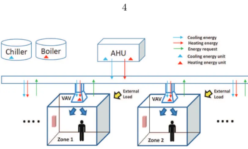
Figure 1.1 Schematic diagram of building energy systems: air handling unit
(AHU) and local zones . . . 4
Figure 2.1 Upper bounds of second order moment ratio as a function of θ and Π and lower bounds of second order moment ratio as a function ofθ . . . . 31
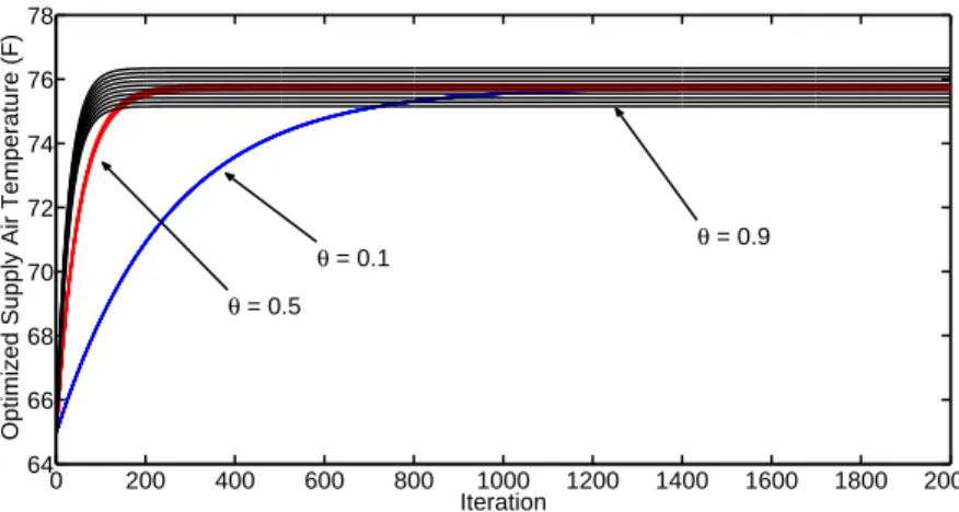
Figure 2.2 Supply air temperature convergence plots with iteration number us-ing different values of control parameterθ; Optimal value 75.8◦F . . . 38
Figure 2.3 Convergence with different values of control parameter . . . 39
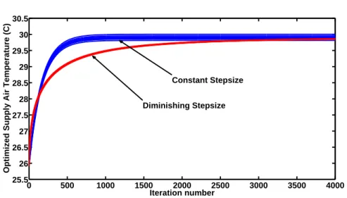
Figure 2.4 Supply air temperature optimization performance with constant step size and diminishing step size . . . 40
Figure 2.5 A partially connected graph consisting of 10 agents (divided into 3 groups); the dashed line indicates weaker connectivity between agents . . . . 40
Figure 2.6 Supply air temperature convergence plots with partially connected graph with constant (left) and diminishing (right) step sizes corresponding toθ= 0.5 . . . 41
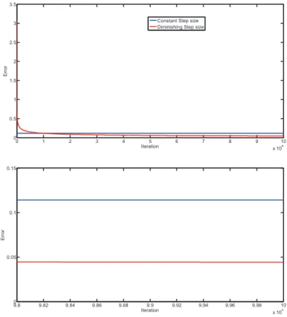
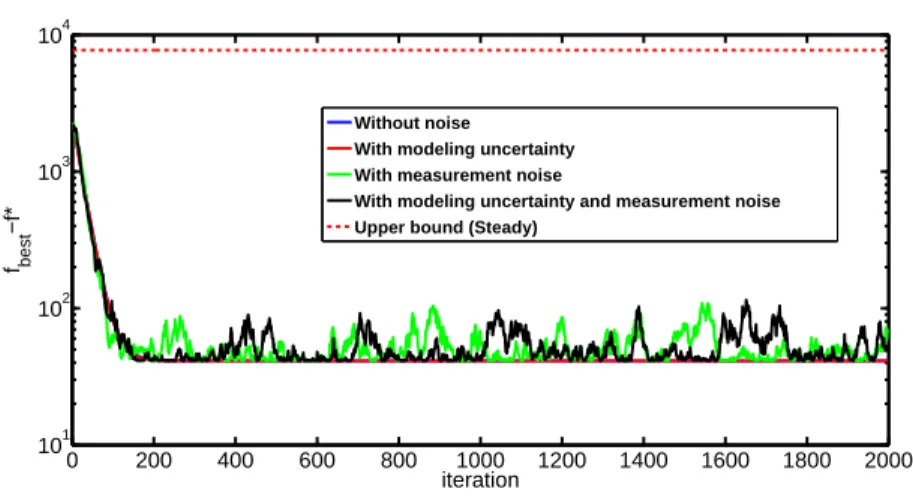
Figure 2.7 Supply air temperature convergence error plots with partially con-nected graph with constant and diminishing step sizes corresponding toθ= 0.5 41 Figure 2.8 Convergence with or without noise . . . 43
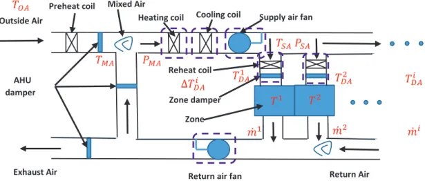
Figure 3.1 Typical layout of an AHU-VAV HVAC system . . . 46
Figure 3.2 Workflow of the proposed supervisory control framework . . . 49
Figure 3.3 Real test bed configuration in Iowa Energy Center . . . 51
Figure 3.4 AHU supply air temperature under supervisory control and baseline control with different outside air temperatures . . . 51
Figure 3.5 Zone temperatures with different outside air temperatures under su-pervisory control . . . 52
Figure 3.6 Total energy consumption in 28 test days in winter . . . 53
Figure 3.7 Energy consumption by cooling/heating coils in AHU, reheat coils at VAVs and power by return/supply fans under supervisory control and baseline control . . . 53
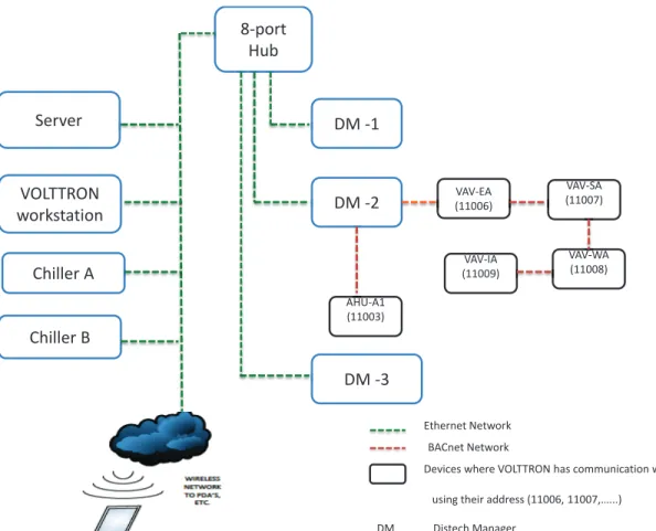
Figure 3.8 Configuration of VOLTTRONTM: there are two networks, i.e., Eth-ernet network and BACnet network; in the EthEth-ernet network, server, VOLT-TRON workstation, chiller A, chiller B, and Distech managers are connected; in the BACnet network, AHU and VAVs are connected . . . 55
Figure 3.9 Software architecture of VOLTTRONTM based implementation: in VOLTTRON, the BACnet Proxy Agent connects the BACnet devices (AHU and VAVs); through the master driver agent, they can publish information to the message bus; other agents can subscribed those published information; the weather agent can also publish and subscribe to the information on the message bus; data from the message bus can also be stored via historian agent 56
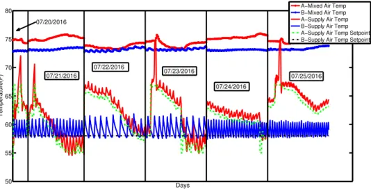
Figure 3.10 Mixed Air Temperature, Supply Air Temperature and Supply Air Temperature Set Point comparison between Systems A and B from 07/20-07/25/2016 . . . 58
Figure 3.11 Mixed Air Temperature, Supply Air Temperature and Supply Air Temperature Set Point comparison between Systems A and B from 07/29-07/31/2016 . . . 58
Figure 3.12 Supply Air Volumetric Flow Rate comparison between Systems A and B from 07/20-07/25/2016 . . . 59
Figure 3.13 Supply Air Volumetric Flow Rate comparison between Systems A and B from 07/29-07/31/2016 . . . 59
Figure 3.14 East Zone Temperature comparison between Systems A and B . . . . 60
Figure 4.2 Fully connected graph, strongly convex case:(a) Convergence rates with differentθwhen α= 0.01 (b) Convergence rates with different θwhen step size is diminishing . . . 73
Figure 4.3 Fully connected graph, strongly convex case: optimization solutions with different θ . . . 74
Figure 4.4 Non-fully connected graph with 3 clusters . . . 74
Figure 4.5 Non-fully connected graph, strongly convex case:(a) Convergence rates with different θ when α = 0.007 (b) Convergence rates with different θwhen step size is diminishing . . . 76
Figure 4.6 Non-fully connected graph, strongly convex case:(a) optimization solutions when α = 0.3, θ = 0.01 (b) optimization solutions when α = 0.3, θ= 0.1 . . . 77
Figure 4.7 Comparison of performance between DGCG and momentum variant of DGCG . . . 78
Figure 5.1 Average training (solid lines) and validation (dash lines) accuracy for (a) comparison of CDSGD with centralized SGD and (b) CDMSGD with Federated average method . . . 97
Figure 5.2 Average training (solid lines) and validation (dash lines) accuracy along with accuracy variance over agents for CDMSGD algorithm with (a) varying network size and (b) varying network topology . . . 98
Figure 5.3 Average training (solid lines) and validation (dash lines) loss for (a) CDSGD algorithm with SGD algorithm and (b) CDMSGD with Federated averaging method . . . 99
Figure 5.4 Average training (solid lines) and validation (dash lines) (a) loss and (b) accuracy for SGD, CDSGD, CDMSGD and Federated averaging method for the CIFAR-100 dataset (c) loss and (d) accuracy for SGD, CDSGD, CDMSGD and Federated averaging method for the MNIST dataset . . . 100
Figure 5.5 Average training (solid lines) and validation (dash lines) (a) loss and (b) accuracy for SGD, MSGD and CDMSGD method for the MNIST dataset for decaying step size. (c) loss and (d) accuracy for CDMSGD for the MNIST data with different learning rates . . . 102
Figure 6.1 A closer look at the optimization updates in distributed deep learn-ing: Blue dots represent the current states (i.e., learned model parameters) of the agents; green dots represent the individual local optima (θi∗), that agents converge to without sufficient consensus; the purple dot (θ∗) repre-sents the ideal optimal point for the entire agent population; another purple dot ˆθrepresents a possible consensus point for the agents which is far from optimal; blue and red curves signify the convergence trajectories with differ-ent step sizes; the green dashed circles indicate the neighborhoods ofθ∗ and ˆ
θ, respectively; d2 represents the consensus bound/error and d1 represents the optimality bound/error; ideally, both of these bounds should be small . 107
Figure 6.2 Performance of different algorithms with unbalanced sample distri-bution among agents. (Dashed lines represent test accuracy & solid lines represent training accuracy.) . . . 127
Figure 6.3 Performance of g-CDMSGD for different ω values. (Dashed lines represent test accuracy & solid lines represent training accuracy.) . . . 128
Figure 6.4 The accuracy percentage difference between the best and the worst agents for different algorithms with unbalanced and balanced sample distri-bution among agents. . . 128
Figure 6.5 The accuracy percentage difference between the best and the worst agents with balanced sample distribution for CDMSGD, i-CDMSGD and g-CDMSGD (varyingω.) . . . 129
Figure 6.6 Performance of different algorithms on balanced and uniformly dis-tributed data among agents. (Dashed lines represent test accuracy & solid lines represent training accuracy.) . . . 130
Figure 6.7 Performance of different non-momentum versions of the algorithms. (Dashed lines represent test accuracy & solid lines represent training accuracy.)131
Figure 6.8 Performance of g-CDMSGD algorithm with different ω values with an unbalanced and non-uniform distribution of data (20% non uniformity). . 131
Figure 6.9 Performance of g-CDMSGD algorithm with different ω values with an unbalanced and non-uniform distribution of data (40% non uniformity). . 132
Figure 6.10 Performance of g-CDMSGD algorithm with different ω values with an unbalanced and non-uniform distribution of data (60% non uniformity). . 132
Figure 6.11 Performance of different algorithms with a balanced data distribution on MNIST dataset . . . 133
ACKNOWLEDGEMENTS
I would like to take this opportunity to express my thanks to everyone who has inspired me and helped me with various aspects in completing this work. First and foremost, I would like to express my sincerest gratitude and appreciation to Dr. Soumik Sarkar for his immeasurable amount of guidance, patience and support throughout my graduate study and research. His insights and words of encouragement are truly a blessing to me and have often inspired me to become an excellent, well-rounded practitioner of science. He is certainly a great advisor, a thoughtful friend, and a role model. I would also like to thank my committee members, Dr. Sourabh Bhattacharya, Dr. Atul Kelkar, Dr. Nicola Elia and Dr. Umesh Vaidya for providing insightful advice, efforts and contributions to this work. I am especially grateful to my family and the Shahs family for constantly offering emotional support while enrolled in the graduate program. I would also like to thank my friends, especially my labmates (they are Kin Gwn Lore, Chao Liu, Adedotun Akintayo, Linjiang Wu, Aaron Havens, Aditya Balu, Sambuddha Ghosal, Venkatesh Chinde, Homagni Saha, Sambit Gadhai, Tryambak Gangopadhyay, Luis G. Riera, Koushik Nagasubramanian, Apurva Kokate, Sin Yong Tan, Lee Xian Yeow, Kai Liang Tan), who have been my close friends to get help from, share the joys of successful achievements and the griefs of having papers rejected for publication. Thank you all for being there with me during both good and bad times, and for making my time as a graduate student extremely delightful and memorable. I would like to thank all of my collaborators, especially Dr. Chinmay Hegde and Dr. Kushal Mukherjee. Without their invaluable opinions and expertise, I would never have produced tangible results from my research efforts. Finally, I would also like to thank my best friend, Dylan Shah, whom I have shared a lot happiness and unhappiness with. Without him, I cannot go “deep”. The work has been supported in part by Iowa Energy Center under Grant No.OG-15-005, National Science Foundation under Grant No.CNS-1464279, USDA-NIFA under Award No.2017-67021-25965.
ABSTRACT
Large scale multi-agent networked systems are becoming increasingly popular in industry and academia as they can be applied to represent systems in diverse application areas, such as intelligent surveillance and reconnaissance, mobile robotics, transportation networks and complex buildings. In such systems, issues related to control and learning have been significant technical challenges to affect system performance and overall cost. While centralized optimization approaches have been widely used by the engineering and computer science community, advanced and effective distributed optimization techniques have not been explored sufficiently and thoroughly in this regard. This study explores various categories of centralized and distributed optimization methods that have been applied or may be applicable for diverse engineering and science problems. The performance of centralized or distributed optimization schemes significantly depends on various factors includ-ing the types of objective functions, constraints, step sizes, and communication networks, etc. In this context, the focus of this dissertation is towards developing novel distributed optimization algorithms in order to solve challenging control and learning problems in various domains such as large-scale building energy systems and robotic networks. Specifically, we develop a general-ized gossip-based subgradient method for solving distributed optimization problems in large-scale networked systems, e.g., larger-scale commercial building energy systems. Different from previous work, a user-defined control parameter is introduced to control a spectrum from globally optimal solution to suboptimal solutions and the trade-off between the solution accuracy and temporal convergence. We test and validate our proposed algorithm on a real testbed involving multiple zones incorporating a distributed control and sensing platform. In addition, we extend the dis-tributed optimization to the deep learning area for solving an emerging topic, i.e., disdis-tributed deep learning, in fixed topology networks. While some previous work exists on this topic, the data par-allelism and distributed computation are still not sufficiently explored. Therefore, we propose a
class of distributed deep learning methods to tackle such issues by combining the consensus pro-tocol and stochastic gradient descent approach. Moreover, to address the consensus-optimality trade-offs in distributed convex and nonconvex optimization, especially in deep learning when the training datasets for agents are non-balanced (non-iid), we propose and develop new approaches in this research, namely, incremental consensus-based distributed stochastic gradient descent and generalized consensus-based distributed (stochastic) gradient descent approach.
CHAPTER 1. INTRODUCTION
Optimization has proved to be an absolutely critical aspect for diverse engineering and science such as control (Boyd and Vandenberghe, 2004), machine learning Sra et al. (2012); Bottou (2010), operation research Rardin and Rardin (1998); Heyman and Sobel (1982), social sciences Borodin et al. (2010) and neural sciences Cochocki and Unbehauen (1993), etc. In both academia and industry, a large variety of optimization methodologies have been proposed and developed to solve numerous real-life problems including but not limited to energy efficiency, economic cost, path planning, optimal control, pattern recognitions, signal processing, etc. Networked systems have attracted considerable attentions recently due to the scales of systems growing significantly. For example, in a large-scale smart building Agarwal et al. (2010), typically there are many zones that have different energy consumption and thermal comfort requirements as well as complicated interactions among them. Moreover, massive amount of available system data that are accessible to customers and researchers are generated and collected every day. Under this situation, con-ventional centralized optimization techniques may not necessarily satisfy the need of networked systems. Therefore, decentralized Raffard et al. (2004) or distributed optimization Boyd et al. (2011) methodologies should be proposed and realized. In distributed optimization, each individ-ual agent state is computed by the combination of its own state and the states from other agents in its neighborhood. This chapter aims at presenting a general introduction and the state-of-the-art on centralized optimization and distributed optimization techniques as well as the objectives of this study.
1.1 Motivation
Many control and machine learning problems can be cast as optimization problems in which some variables of interest are optimized to minimize some cost such as energy cost, time cost, or economic cost (in controls) and error between ground truth and inference results (in machine
learning). For instance, in a large-scale commercial building, improving the energy efficiency in the heating, ventilation, and air-conditioning system, and maintaining the different zone comfort requirements would require reducing the energy consumption and minimizing the difference be-tween actual zone temperature and reference temperature (or temperature set point), respectively. Moreover, in predictive modeling Kuhn and Johnson (2013), finding a hypothesis or model that can establish the relationship between the input and the output typically requires minimizing the mean-square errors between actual and predicted outputs. In summary, optimization techniques are critically important in controls and machine learning and can affect the performance of relevant models. Among several possible engineering or science applications, this study focuses on propos-ing and developpropos-ing novel distributed optimization algorithms for control problems (i.e., large-scale smart building energy systems for improving energy efficiency and maintaining thermal comfort requirements) and machine learning problems (i.e., deep neural networks for improving leaning ability). While these problems come from different areas, this study will aim to show the effec-tiveness of similar distributed optimization algorithms in order to obtain state-of-the-art results in their respective disciplines. The main elements of the hypothesis that this study will focus on are described by the following general questions. What distributed optimization problems are consid-ered? How can these distributed optimization problems be extended? What algorithms should be considered in terms of different problems? How do these algorithms perform? What improvement can be made on the algorithm performance? Questions of these kinds are almost always quite difficult to answer because they depend largely on the problem at hand.
1.2 Project Goals
The distributed algorithms for tackling these kind of problems are generally non-trivial. How-ever, the appeal for them are due to their scalability and robustness in different applications. For example, in large scale building energy systems, most problems of these kinds are complex and would require optimal set points to improve energy efficiency as now most of such systems do not take into account the optimal energy consumption, but only considering the thermal comfort re-quirements. Also, centralized control or optimization for building energy systems cannot satisfy
the requirements by large-scale building energy systems since it may be significantly difficult to effectively establish a large-scale model and then solve the problem. For most of the deep learning problems, centralized techniques are still popular due to the complexity (e.g., nonlinearity and nonconvexity) of problems. However, as the sizes of model and data grow exponentially, paral-lel or distributed approaches of deep learning have received considerable attention and should be developed accordingly. Therefore, the entire pipeline requires efficient distributed optimization al-gorithms to extend the existing centralized techniques and solve the problem itself effectively. This is the main motivation of the present research work where the goal is to develop distributed opti-mization algorithms for large-scale building energy systems and parallel deep learning models for intelligent decision-making and inference processes. This study will show different methodologies that have been developed for controls and machine learning, as well as their shortcomings and im-provements made. Some of specific applications in large-scale building energy systems and machine learning problems investigated in this study are described in the following subsections.
1.2.1 Large-scale Building Energy Systems
The scale of modern commercial buildings is significantly large with many local zones requiring various thermal comfort requirements. The general layout of the air-side HVAC system in buildings is shown in Figure 1.1. In such a system, due to the different requirements from local zones, the supply air temperature is typically set constant and low, which may waste a large amount of energy. Previous work has also been done using distributed model predictive control (DMPC) Camponogara et al. (2002), which may require the complex physical models for the thermal dynamics of each local zone. In this study, to deal with the issue of local thermal dynamics, we seek to use data-driven methods to avoid establishing the complex physical relations among different variables. A distributed optimization algorithm is proposed and developed to minimize the total energy consumption and to maintain the thermal comfort requirements from local zones between a pre-specified temperature band.
Figure 1.1: Schematic diagram of building energy systems: air handling unit (AHU) and local zones 1.2.2 Deep Learning Models
As a branch of machine learning, deep learning has been gradually becoming a standard tech-nique to solve numerous problems, including computer vision LeCun et al. (2015), natural language processing Collobert and Weston (2008), finance Heaton et al. (2017), physics Baldi et al. (2014); Lore et al. (2018); Stoecklein et al. (2017); Akintayo et al. (2016), and transportation Ma et al. (2015); Chakraborty et al. (2018). As the sizes of data and model become massive, distributed deep learning approaches ) that have been investigated for improving the computational efficiency should be developed for larger scales of problems. However, most existing methods impose strong assumptions on objective functions which limit the applications of those proposed algorithms. Also, the proposed schemes typically introduce a center variable which plays a critical role as a param-eter server. In practice, central paramparam-eter server may be failed or unavailable resulting in the failure of the proposed algorithms. The data distribution is another critical issue that can affect the performance of models. In the existing work, one generic assumption that is made for most of algorithms is that the sampling data is independently identical and distributed (iid), which is not necessarily the case in most of real-world problems. In this work, we propose a class of distributed algorithms that can be applied to any deep learning models and do not rely on the center parameter server. Such methods are also shown to handle non-iidness in data better than other traditional approaches.
1.3 Aims and Objectives
The objective of this research is to develop the distributed optimization algorithmic frameworks for improving energy efficiency and maintaining thermal comfort requirements in large-scale build-ings by determining the optimal temperature set points, realization of distributed deep learning under data parallelization setting without the center parameter server, and addressing the issue. The first application is a control and optimization problem for building energy systems to reduce the energy consumption and satisfy the comfort requirements. This will help building tenants or managers make intelligent decisions. The second application is in the field of deep learning - par-allelize the existing deep learning models in networked systems with data parallelization to aid in solving large-scale deep learning problems. In addition to these applications, the overarching aim is to explore the performance (e.g., convergence rate and accuracy) of proposed algorithms.
The aims and significant contributions of the study are outlined as follows:
1. to propose and develop novel distributed optimization algorithms and establish the algorith-mic frameworks
2. to provide rigorous theoretical analysis on different distributed optimization algorithms pro-posed in this study
3. to compare the proposed algorithms with state-of-the-art methods for validation
4. to apply the proposed algorithms to specific controls and leaning problems in large-scale networked systems
5. to analyze and discuss the results obtained from applications of the algorithms to real-world problems
1.4 Related Work
In this section, the available wealth of knowledge that builds up to developing the technique are summarized. The basic concepts of optimization and deep learning and literature on the centralized optimization are kept in the background.
1.4.1 Distributed Optimization in Controls
Large scale multi-agent networked systems are popular in industry and academia as they can be applied to various areas, such as intelligent surveillance and reconnaissance, mobile robotics, transportation networks and complex buildings (Jadbabaie et al., 2006; Patterson et al., 2010; Saber et al., 2007). These networked systems consist of a large number of sensors and actuators that can be regarded as interacting agents, which communicate and exchange information with other agents such that a global perspective of phenomenon is observed. In distributed optimization problems for multi-agent networked systems, autonomously optimizing the behaviors of agents or allocating resources within such sensor and actuator networks without consuming large amount of computational and economic cost remains a technical challenge. The current state-of-the-art techniques to overcome such a challenge is to apply cooperative and non-cooperative (Altman et al., 2007) distributed optimization (Tsitsiklis et al., 1986) to the best agent behavior or resource allocation. These methods yield a global decision that is shared by all agents in order to prevent local minima (Borkar and Varaiya, 1982).
Subgradient methods (Boyd et al., 2003; Nedic and Ozdaglar, 2009; Nedic and Bertsekas, 2008; Yuan et al., 2011; Long et al., 2015; Nedic and Ozdaglar, 2008) have been broadly used to iter-atively refine the estimates of the shared decision for each agent in a distributed manner. The difference between gradient and subgradient is that subgradient methods can be extendedly ap-plied to optimization problems with nondifferentiable cost functions. Furthermore, the necessary conditions for subgradient methods are relaxed compared to the gradient methods. In (Johansson et al., 2008), a scheme combining consensus algorithm with subgradient method was presented for solving the convex optimization problems. In (Saber et al., 2007), a theoretical framework was established for consensus and cooperation in networked multi-agent systems, and in (Nedic and Ozdaglar, 2009) the distributed subgradeint methods were developed for multi-agent optimization. Moreover, in (Nedic and Ozdaglar, 2008) the authors also provided the analysis of estimates for convergence rate that the function value converged to the primal optimal value within an error at a rateO(1/k) in the number of subgradient iterationsk. Some other methods such as approximated subgradient (Kiwiel, 2004), incremental subgradient (Nedic and Bertsekas, 2001b), and stochastic
subgradient methods (Ram et al., 2008) were also proposed and developed for large-scale distributed optimization problems.
“Agreement” or “consensus” is one of the most widely used concept in the area of multi-agent systems for information fusion, decision-making, information propagation and distributed opti-mization. Among various protocols, gossip-based consensus algorithms (Franceschelli et al., 2010) are quite popular due to their simple nature yet powerful properties as well as strong analytical results (Shah, 2008; Salehi Tahbaz and Jadbabaie, 2010). Recently, gossip algorithms (Ram et al., 2009; Lu et al., 2010) were extended to generalized gossip algorithms (Sarkar et al., 2013) such that the entire spectrum from “complete consensus” to “complete disagreement” can be obtained. In (Sarkar et al., 2013) a tradeoff was characterized to vary the dissemination of agent beliefs throughout the network between the decision propagation radius (i.e., how far a decision spreads from its source) and localization of information. Compared with pure consensus algorithms, gener-alized gossip algorithms aim at describing the observed phenomenon at more ‘local’ level in sensor and actuator networks as the proximal agents are more likely to share similar beliefs while the consensus of the belief state of agents is not guaranteed. This paper explores the effects of such a generalized time-synchronous gossip protocol on subgradient based distributed optimization. The optimal solution is derived from performing a more ‘local’ consensus of behavior or allocation of resources. With a user-defined generalizing parameter in the agent interaction policy, the trade-off between propagation radius and localization gradient may be controlled to yield a spectrum of optimal solutions ranging from globally optimal solution (complete consensus) to greedy locally op-timal solution (no compromise). The generalized gossip-based subgradient optimization algorithm is applicable to networks with multiple (possibly non-collocated) resources and consumption enti-ties. Examples of such networks include power grid, transportation networks and building energy distribution networks (Atzeni et al., 2013).
This study also takes into account the noise in a networked system in which subgradient es-timates and agent communication may be noisy such that the global optimal solution cannot be accurately reached. In the literature, Nedic et al (Nedic and Bertsekas, 2008) considered the ef-fect of deterministic and bounded noise in subgradient methods by the introduction of noise of
subgradients and function values. Srivastava et al (Srivastava et al., 2010; Srivastava and Nedic, 2011) provided a distributed algorithm for the case when there was communication noise present in networks, and furthermore established sufficient conditions for the convergence. In (Nedic and Lee, 2014) the authors proposed a stochastic subgradient mirror-descent method with weighted iterate-averaging and analyzed its covergence rate. The authors in (Cavalcante and Stanczak, 2013) devised and analyzed a novel distributed online algorithm for dynamic optimization prob-lems in noisy communication environments. Noisy links have been taken into account as well over networks in other related works (Touri and Nedic, 2009; Kar and Moura, 2009) where asymptotic convergence results were established. Motivated by the previously related work, this paper assumes that there are mainly two kinds of noise existing in a networked system. They are the modeling uncertainty associated with subgradient estimations and the measurement noise associated with agents. This paper presents the effects of such noise types on the function value error bounds.
1.4.2 Applications to Large-scale Building Energy Systems
Today, the building sector accounts for approximately 40% of the total energy usage in the U.S. (residential 22%, commercial 18%) E08 (2008). Therefore, energy-efficient building technology is significantly critical for large-scale buildings. The performance of heating, ventilation, and air-conditioning (HVAC) systems have a significant impact on the building energy consumption. In order to address this issue, a vast number of different control and optimization techniques have been developed to minimize energy consumption while maintaining zone comfort requirements.
Model predictive control (MPC) and its variants have been commonly used to minimize the energy consumption. Scherer et al Scherer et al. (2014) proposed a distributed model predictive control (DMPC) scheme for the efficient management of energy distribution in buildings. Razmara et al Razmara et al. (2015) provided an exergy model using MPC technique and the simulation results showed the advantage of XMPC over conventional energy-based MPC. Liang et al Liang et al. (2015) combined the auto-regressive moving average exogenous model (ARMAX) with MPC technique to minimize the energy consumption in air handling unit (AHU). Evolutionary algorithms such as genetic algorithms were employed for optimizing building energy consumption Yang et al.
(2014); Wright et al. (2002); Evins (2015); Magnier and Haghighat (2010). Accurately capturing the thermal dynamics associated with building zones is significantly challenging and time-consuming as they are exposed to disturbances and uncertainties, such as occupancy, weather etc. In Menassa et al. (2014), a framework is proposed to optimize building energy consumption by combining dis-tributed energy simulation tools and occupancy models and they also evaluated energy saving based on occupancy interventions Azar and Menassa (2014). Furthermore, various other policies were also proposed and developed for building energy efficiency, such as optimal energy cost analysis Fer-rara et al. (2014), metamodeling energy consumption needs and simultaneous building envelop optimization Ronami et al. (2015), robust optimization approach Liu and Fu (2013), use of a ran-dom number generator Hasan et al. (2014), self-adaptive optimization methods Ramallo-Conzalez and Coley (2014), two-stage optimization Gruber and Prodancovic (2014), collaborative energy and thermal comfort management through distributed consensus algorithms Gupta et al. (2015b), event-based optimization within the Lagrangian relaxation framework Sun et al. (2015), Sun et al. (2013), and a mixed integer model for a small building cluster Yan et al. (2014).
While MPC based schemes are highly dependent on the underlying model, R-C network models which are commonly used to represent thermal zones becomes complicated as the building size grows. On the other hand, heuristic algorithms require a large amount of data collected in order to yield good models. Furthermore, some methods in a centralized manner may not be practically implemented as they rely on a large number of physical variables to establish complex models. Large-scale complex building systems can be represented as multi-agent networked systems for op-timal coordination among different components of HVAC system. Yang and Wang (2011) proposed a multi-agent control method with an intelligent optimizer for building control problems. Wang et al. (2010) applied hierarchical multi-agent theory and Particle Swarm Optimization (PSO) in smart and energy-efficient buildings. Chen et al. (2014) developed a data-driven agent-based com-putational model for energy consumption behavior and they found the major structural parameters that impacted building occupants’ conversation decisions. Cai et al. (2015) also proposed a hier-archical multi-agent method to find the optimal setpoints by using consensus-based optimization algorithms.
1.4.3 Distributed Optimization in Deep Learning
Scaling up deep learning LeCun et al. (2015) is becoming increasingly crucial for large-scale applications where the sizes of both the available data as well as the models are massive Gupta et al. (2015a). Among various algorithmic advances, many recent attempts have been made to parallelize stochastic gradient descent (SGD) based learning schemes across multiple computing agents. An early approach called Downpour SGD Dean et al. (2012), developed within Google’s
disbelief software framework, primarily focuses on model parallelization (i.e., splitting the model
across the agents). A different approach known as elastic averaging SGD (EASGD) Zhang et al. (2015a) attempts to improve perform multiple SGDs in parallel; this method uses a central parame-ter server that helps in assimilating parameparame-ter updates from the computing agents. However, none of the above approaches concretely address the issue ofdata parallelization, which is an important issue for several learning scenarios: for example, data parallelization enables privacy-preserving learning in scenarios such as distributed learning with a network of mobile and Internet-of-Things (IoT) devices. A recent scheme called Federated Averaging SGD McMahan et al. (2016) attempts such a data parallelization in the context of deep learning with significant success; however, they still use a central parameter server.
In contrast, deep learning with decentralized computation can be achieved via gossip SGD algorithms Blot et al. (2016); Jin et al. (2016), where agents communicate probabilistically without the aid of a parameter server. However, decentralized computation in the sense of gossip SGD is not feasible in many real life applications. For instance, consider a large (wide-area) sensor network Mukherjee et al. (2011); Liu et al. (2017) or multi-agent robotic network that aims to learn a model of the environment in a collaborative manner Choi and How (2010); Jha et al. (2016). For such cases, it may be infeasible for arbitrary pairs of agents to communicate on-demand; typically, agents are only able to communicate with their respective neighbors in a communication network in a fixed (or evolving) topology.
Apart from the algorithms mentioned above, a few other related works exist, including a dis-tributed system called Adam for large deep neural network (DNN) models Chilimbi et al. (2014) and a distributed methodology by Strom (2015) for DNN training by controlling the rate of
weight-update to reduce the amount of communication. Natural Gradient Stochastic Gradient Descent (NG-SGD) based on model averaging Su and Chen (2015) and staleness-aware async-SGD Zhang et al. (2015b) have also been developed for distributed deep learning. A method called Cen-tralVR De and Goldstein (2016) was proposed for reducing the variance and conducting parallel execution with linear convergence rate. Moreover, a decentralized algorithm based on gossip proto-col called the multi-step dual accelerated (MSDA) Scaman et al. (2017) was developed for solving deterministically smooth and strongly convex distributed optimization problems in networks with a provable optimal linear convergence rate. A new class of decentralized primal-dual methods Lan et al. (2017) was also proposed recently in order to improve inter-node communication efficiency for distributed convex optimization problems. To minimize a finite sum of nonconvex functions over a network, the authors in Hajinezhad et al. () proposed a zeroth-order distributed algorithm (ZENITH) that was globally convergent with a sublinear rate.
1.4.4 Trade-offs Between Consensus and Optimality
In the control area, numerous research works Boyd et al. (2003); Nedic and Ozdaglar (2009); Nedic and Bertsekas (2001a); Yuan et al. (2011); Long et al. (2015); Jiang et al. (2015a) have been performed for distributed optimization associated with multi-agent networked systems with a focus on finding the globally optimal solution. Locally optimal solutions were achieved for the non-convex optimization problems in a distributed manner Sun et al. (2016); Zhu and Mart´ınez (2013); Bian et al. (2016); Guo et al. (2016). However, many practical problems (e.g., distributed resource allocation applications - building-to-grid control and renewable integration, distributed sensing applications - weather forecast, smart grid monitoring, distributed decision-making in multi-agent robotics with partial information), which may or may not be convex, may require multiple local optimal solutions that are useful for local sub-groups of agents. For instance, consider a large multi-source, multi-destination supply-demand optimization problem, where the goal is to find optimal supply rate(s) to satisfy the needs of the demand side agents. However, the demand side agents can form multiple distinct sub-groups based on their similarities/differences in requirement and one globally optimal supply rate may not be useful in order to satisfy drastically different individual
agent needs. Therefore, it may be more useful to recognize that partition in the overall system and obtain different optimal supply rates and connect different supply sources to different ‘groups’ or ‘clusters’ of demand agents. Few of previous works have reported the trade-offs between the consensus and disagreement in the distributed optimization.
In the deep learning area, a large literature has emerged that studies distributed deep learning in both centralized and decentralized settings Dean et al. (2012); McMahan et al. (2016); Zhang et al. (2015a); Blot et al. (2016); Jin et al. (2016); Xu et al. (2017); Zheng et al. (2017); Zhang et al. (2017), and we only summarize the most recent work. Wangni et al. (2017) propose a gra-dient sparsification approach for communication-efficient distributed learning, while Wen et al. (2017) propose the concept of ternary gradients to reduce communication costs. Scaman et al. (2017) propose a multi-step dual accelerated method using a gossip protocol to provide an optimal decentralized optimization algorithm for smooth and strongly convex loss functions. Decentralized parallel stochastic gradient descent Lian et al. (2017) has also been proposed.
Perhaps most closely related to this study is the work of Berahas et al. (2017), who present a dis-tributed optimization method (calledDGDτ) to enable consensus when the cost of communication is cheap. However, the authors only considered convex optimization problems, and only study de-terministic gradient updates. Also, Qu and Li (2017) propose a class of (dede-terministic) accelerated distributed Nesterov gradient descent methods to achieve linear convergence rate, for the special case of strongly convex objective functions. In Tsianos and Rabbat (2012), both deterministic and stochastic distributed were discussed while the algorithm had no acceleration techniques. To the best of our knowledge, none of these previous works have explicitly studied the trade-off between consensus and optimality.
1.5 Summary
In summary, it can be concluded that there are still significant gaps in extending the centralized optimization schemes to distributed optimization in both controls and machine learning. This chap-ter has taken a bird’s-eye view to identify best-performing competitive architectures for addressing control and learning problems.
CHAPTER 2. GENERALIZED GOSSIP-BASED SUBGRADIENT METHOD
In this chapter, we present a novel distributed optimization algorithm called generalized gossip-based subgradient method along with analysis and validation results.
In large-scale building energy systems, we consider optimizing the temperature set points which typically in a constrained range due to the capacities of actuators and sensors. Therefore, for the control part, constrained distributed optimization problems are investigated accordingly. Since we have different types of distributed optimization problems for both controls and learning, the problems will be formulated separately in order to distinguish diverse work although they share some similarities. Before presenting the specific problem formulations, we discuss the spectral graph theory for the networked systems.
2.1 Spectral Graph Theory
For the rest of this study, we consider an static undirected graph G = (V,A) consisting of N agents which is assumed to be connected, whereV ={1,2, ..., N}andA ⊆ V × V. If (j, l)∈ A, then Agentj can communicate with Agentl, and vice versa. We define the neighborhood of agentj∈ V
asN b(j) ,{j∈ V : (j, l) ∈ Aorj =l}. For such a networked system, we impose the assumption to its corresponding graph as follows which assists in characterizing the main results in this work. Let Π∈RN×N be the agent interaction matrix which signifies the transition probabilities that each
agent communicates with other agents in its neighbor. For example,πjl represents the probability
Assumption 1 • If (j, l)∈ A/ , πjl= 0
• Π = ΠT
• Null{I −Π}= Span{1}
• I Π −I
where1 is the row vector with entries being 1. It can be suggested from the Assumption 1that Π is doubly stochastic and the second largest eigenvalue λ2<1. For the rest of this dissertation, we denote the z-th largest eigenvalue byλz.
Now we are ready the state the problem formulation of constrained distribute optimization.
2.2 Problem Formulation for Constrained Distributed Optimization
This section presents the problem statement and some background knowledge that serves to characterize the main results in constrained distributed optimization. Let a distributed optimization problem be defined on the network as follows:
minimizef(x) = N X j=1 fj(x) subject tox∈ X :=∩Nj=1Xj (2.1)
wherefj :R−→Rare agent level convex objective functions that are not assumed to be differen-tiable. Xj are different nonempty, closed, bounded and convex subsets of
R. Each local objective functionfj and constraint setXj are only known to the node j.
2.2.1 Preliminary Background
The basic definitions (Boyd et al., 2003; Johansson et al., 2008) and assumptions used in this paper are:
Definition 2 g∈R is a subgradient of a convex functionf :R−→R at a point z∈R if
Definition 3 The set of all subgradients of a convex functionf atz∈Ris called the subdifferential
of f at z, and is denoted by ∂f(z):
∂f(z) ={g∈R|f(y)≥f(z) +g(y−z),∀y ∈R} (2.3)
Definition 4 g is a-subgradient if ∃≥0, for all y∈R, f(y)≥f(z) +g(y−z)−.
Assumption 5 (Subgradient boundedness):There exists a scalar G ≥0 for all j = 1, ..., N, such that
|g| ≤G,∀g∈∂fj(x),∀x∈ X (2.4)
Assumption 6 The optimal solution set X∗ is nonempty.
In the area of distributed optimization, subgradient methods have played a critical role as they enable decentralized formulations. The standard distributed subgradient formulation for multi-agent distributed optimization (see (Nedic and Ozdaglar, 2009)) is as follows:
xjk+1=
N X
l=1
ajlkxlk−αjkdjk (2.5)
where ajl are weights, αjk are stepsizes, dkj are the subgradients of fj at xjk and k is a time index. Depending on choice of weights, this formulation has been shown to solve multi-agent optimization problems primarily via consensus. Choice of step size is also key to obtain desired convergence properties.
2.2.2 Generalized Gossip Algorithm
In the context of distributed information propagation in a mobile sensor network (Sarkar et al., 2010), the present authors proposed a generalized gossip protocol (Sarkar et al., 2013). Furthermore, a power-aware extension of the agent interaction policy was proposed more recently that conserves sensor power when there is no point of interest and the sensors become active in an event-triggered manner (Sarkar and Mukherjee, 2014). Similar concept was also used to generate a belief map to guide an autonomous robot to the source in a GPS-denied environment (Chattopadhyay et al.,
2015). One of the key observations made in these studies was that a user defined parameter is able to control the fundamental tradeoff between information propagation radius and localization gradient. In other words, the tradeoff was between “degree of consensus” and “degree of disagreement”. This paper explores this formulation for a distributed optimization problem where the tradeoff is between “global optimal” achieved through compromise and “local optimal” (s) achieved in a greedy manner by individual agents. The terminology ‘generalized gossip’ also appears in a few other recent papers. For example, Matei et. al. (Matei et al., 2014) generalized the notion of convex metric spaces in the context of distributed optimization using random gossip (Boyd et al., 2006) consensus algorithms. However, a similar tradeoff appears in the formulation as agents choose between own state and neighbors’ states during update. In a different context, the generalized gossip terminology has been used to obtain communication protocols in the spectrum strict gossip and broadcast policies (Khuller et al., 2003).
The generalized gossip protocol outlined in (Sarkar et al., 2013) for belief propagation in a mobile sensor network is as follows:
υjθk+1 = (1−θ) X
l∈N b(j)
πjlkυθkl +θχ
j
k (2.6)
whereθ∈(0,1] is a user-defined control parameter, N b(j) is the set of agents in the neighborhood of agent j. In this set, agents can communicate with agent j during the time span between k and k+ 1. Agent interaction matrix Π = I −βL (Sarkar et al., 2013), where L = D−A, D is the degree matrix, A is the adjacency matrix. β is an appropriately chosen constant. υ and χ are the vectors representing agent belief measure and state characteristics function (quantikfying observations made by agents), respectively. While the agent interaction matrix may in general be time varying, it maintains thedoubly stochastic property. As mentioned above, it has been shown that the user-defined control parameter θ∈(0,1] can be chosen appropriately to achieve a desired tradeoff between “degree of consensus” and “degree of disagreement”. Further details can be found in (Sarkar et al., 2013).
In the present context, agents can exchange information synchronously (Xiao and Boyd, 2004; Dimakis et al., 2010) or asynchronously (Ram et al., 2009). While our algorithm can perform
sufficiently well under asynchronous updates, we use the synchronous update scheme in this paper for analytical simplification. Therefore, we have the following assumption.
Assumption 7 (Synchronous Communication): Each agent communicates with other agents in its neighborhood synchronously.
2.3 Generalized Gossip-based Subgradient Algorithm
In this section, the generalized gossip-based subgradient algorithm is proposed for distributed optimization. The static graph is considered such that the weight matrix is time-invariant. In this formulation, the discrete-time update law (derived from eqn. 2.5 and 2.6) for the optimization variable is as follows: xjk+1=PX[(1−θ) X l∈{j}∪N b(j) πjlxlk+θ(x j k−αk∇ j k)] (2.7)
where ∇jk is the subgradient of fj at xjk computed by agent j, αk is the step size which can be
constant or diminishing, PX[˜x] is the Euclidean projection of any point ˜x onto the constraint set
X, i.e., PX = argmin x
|x−x˜|,∀x∈ X.
In a vector notation, the update rule becomes:
xk+1 =PX[(1−θ)Πxk+θ(xk−αk∇k)]. (2.8)
It should be noted that this policy boils down to a standard consensus-based optimization protocol using subgradients when the control parameter θ approaches 0. On the other hand, as θ approaches 1, interaction among agents reduces significantly and individual agent-level optimization variables tend to converge to their respective local minima based on individual subgradients. Formal discussion on this aspect will follow the analytical results presented in the sequel.
Remark 8 The advantage of the generalized gossip-based method is to provide a tradeoff between consensus and disagreement among agents in a networked system. The user-defined control param-eter plays a critical role in controlling such a tradeoff as well as the temporal convergence. Under this scheme, a spectrum of solutions can be obtained ranging from the globally optimal solution
(complete consensus) to greedy suboptimal solutions (complete disagreement). However, we note that such suboptimal solutions can still be interesting in the sense of being optimal with respect to a single agent or a smaller group of agents as we discuss in the sequel. The temporal convergence is also significantly faster when greedy solutions are sought. Therefore, the framework provides a useful flexibility of selecting the tradeoff between degree of suboptimality and convergence time. This methodology can be effectively applied to many practical problems (e.g., distributed resource alloca-tion applicaalloca-tions building-to-grid control and renewable integraalloca-tion, distributed sensing applicaalloca-tion weather forecast, smart grid monitoring, distributed decision-making in multi-agent robotics with partial information).
Both convergence analysis of first and second statistical moments are required for understanding the implications of the proposed protocol. Therefore, based on (Jiang et al., 2015b), this paper presents analytical results for the first and second moments along with generic numerical results. Following are notations and lemmas required for the convergence analysis.
For first moment analysis, ensemble average (over agents) ofxk and∇k are denoted by ¯xk and
¯
∇k respectively. They are defined as:
¯ xk= 1 N1 Tx k= 1 N N X j=1 xjk (2.9) ¯ ∇k= 1 N1 T∇ k= 1 N N X j=1 ∇jk (2.10)
where1 is a column vector with all elements being 1.
Note, multiplying the update rule described in eqn.2.8by N11T yields the following relationship (as Π is doubly stochastic):
¯
xk+1=PX[¯xk−θαk∇¯k] (2.11)
The form of this equation is similar to that of the projected subgradient method.
Next, optimal function values are denoted by f∗, that are assumed to be finite. Without loss of generality the optimal set is represented byX∗, i.e., X∗ ={x∈ X |PN
j=1fj(x) =f∗}. Here are a few necessary lemmas required for convergence analysis.
Lemma 9 If assuming that |xik−xjk| ≤σ<∞,∀j, l= 1, ..., N, then |xjk−x¯k| ≤σ.
See (Johansson et al., 2008) for proof.
Note, this lemma suggests that if pairwise distance between optimization variables of any two agents is bounded then distance between the average and any point is bounded by the same quantity.
Lemma 10 If Assumption 5 holds, then for a sequence {∇¯k}, ∀k,
|∇¯k| ≤G.
See (Jiang et al., 2015b) for proof.
This lemma suggests that if all individual agent level subgradients are bounded, then the average subgradient is also bounded by the same quantity.
Lemma 11 If Assumption 5 holds, then, for a sequence {x¯k},∀kand z∈R,
f(z)≥f(¯xk) +N∇¯k(z−x¯k)− (2.12)
where = 2N Gσ.
See (Jiang et al., 2015b) for proof.
Note, Lemma 11 shows thatN∇¯ is an-subgradient of ¯x.
2.4 Convergence Analysis
2.4.1 First Order Convergence Analysis
In this section, we present the first moment analysis for the proposed algorithm. The analysis begins with the following lemma.
Lemma 12 If Assumptions 5-7 hold, then, for a sequence{x¯k}, ∀k,
|x¯k+1−x∗|2≤ |x¯k−x∗|2−2θαk
1
N(f(¯xk)
−f∗) + 4θGσαk+θ2G2α2k.
Proof. (Sketch): First replace ¯xk+1 with the update law and then use the nonexpansiveness property of Euclidean projection on a convex set to get the |x¯k+1 −x∗|2 ≤ |x¯k−θαk∇¯k−x∗|2.
Second, use the Assumptions5-6, Lemma 9, Lemma10, and Lemma11 to get the desired result.
Lemma12suggests that ¯xgets closer tox∗with every iteration whenf(¯x) is much greater than f∗. However, asf(¯x) comes very close to f∗, ¯x is not guaranteed to get closer tox∗. This is due to the two terms in the equation, 4θGσαk andθ2G2α2k. If the control parameterθis reduced, then
the terms reduce in magnitude and ¯x approachesx∗.
Next, Theorem 13 is introduced to provide an upper bound for the optimized function value. Theorem 13 If Assumptions5-7 hold, then, for a sequence{xkj},∀k andj= 1, . . . , N, when step
size αk=α, f(xjk)min≤f∗+ N|x¯(1)−x∗|2 2mθα +3N Gσ+N θG 2α 2 (2.14)
where f(xjk)min= min{f(xj(1)), . . . , f(xj(m))}, m is the number of iterations.
As the subgradient is not always in the descent direction, the best value needs to be tracked that best approachesf∗. Hence, after m iterations, the best value is denoted by f(xjk)min.
Proof. Recalling the conclusion of Lemma 12, as step sizeαk =α, the following relation can
be obtained |x¯k+1−x∗|2 ≤ |x¯k−x∗|2−2θα 1 N(f(¯xk) −f∗) + 4θGσα+θ2G2α2. (2.15)
Applying the above inequality recursively form iterations, then we can obtain
|x¯m+1−x∗|2 ≤ |x¯1−x∗|2−2θα 1 N m X k=1 (f(¯xk)−f∗) 4mθGασ+mθ2G2α2 (2.16)
As|x¯m+1−x∗|2 ≥0, the last inequality can be rewritten as 0≤ |x¯1−x∗|2−2θα 1 N m X k=1 (f(¯xk)−f∗) + 4mθGασ+mθ2G2α2 (2.17)
As 2θαN1 Pm
k=1(f(¯xk)−f∗)≥2θαN1
Pm
k=1mink=1,2,...,m(f(¯xk)−f∗), then we have that
2θα1 N m X k=1 mink=1,2,...,m(f(¯xk)−f∗)≤ |x¯1−x∗|2 + 4mθGασ+mθ2G2α2 (2.18) which leads to f(¯xk)min−f∗ ≤ N|x¯(1)−x∗|2 2mθσ + 2N Gσ+ N θG2α 2 (2.19)
Based onfi(¯xk)≥fi(xjk)+∇j(¯xk−xjk) we can know that using Assumption5,f(xkj)≤f(¯xk)+N Gσ,
which is combined with the last inequality to get the desired result.
Theorem 13 demonstrates the convergence of function values and it can be concluded that for a givenθ, as number of iteration mincreases, the upper bound converges to f∗+ 3N Gσ+N θG22α. Thus,f(xjk)min converges within 3N Gσ+N θG
2α
2 from the optimal value. Also, note that effect of initial condition dies out with a large value of m.
Roughly, asθapproaches 0, the last term on the right hand side of eqn.2.14vanishes. Also, for an arbitrarily small θ, one can always find a large m for which the second term on the right hand side of eqn.2.14vanishes. Therefore, asθ→0,f(xjk)min converges within 3N Gσ from the optimal
value.
Next, the convergence characteristics are analyzed as the step size αk diminishes.
Let a sequence {αk}, k= 1,2, . . . , mbe defined as follows.
Definition 14 {αk} is a sequence that satisfies the following properties:
(1): αk is positive; (2): αk converges to 0; (3): {αk} is a nonsummable sequence. Hence, αk≥0; lim k→∞αk= 0; mlim→∞ m X k=1 αk=∞. (2.20)
and there exists an integer N1, that satisfies
αk≤
δ
Then there exists another integerN2 such that m X k=1 αk≥ 1 δθ(N|x¯1−x ∗|2+N G2θ N1 X k=1 α2k),∀m>N2.
This inequality holds because limm→∞Pmk=1αk=∞.
Now, let N=max{N1, N2}, and the following Theorem15 can be stated.
Theorem 15 If Assumptions5-7 hold, then, for a sequence {xjk}, ifαk satisfies Definiton 14, ∀k,
and j= 1, . . . , N,
f(xjk)min ≤f∗+δ+ 3N Gσ,∀m>N. (2.22)
where f(xjk)min= min{f(xj1), . . . , f(x
j
m)}, δ is an arbitrarily small nonnegative constant.
Proof. According to Theorem 13, we can obtain that
f(xjk)min−f∗≤
N|x¯1−x∗|2+ 6NPmk=1αkθGσ+N G2θ2Pmk=1α2k
2θPm k=1αk
(2.23)
then rewriting the above inequality,
f(xjk)min−f∗ ≤ N|x¯1−x∗|2+N G2θ2 PN1 k=1α2k 2θPm k=1αk +6N Pm k=1αkGσ 2Pm k=1αk + N G 2θPm k=N1+1α 2 k 2PN1 k=1αk+ 2 Pm k=N1+1αk ≤ N|x¯1−x ∗|2+N θ2G2PN1 k=1α2k 2 δ[N|x¯1−x∗|2+N θ2G2 PN1 k=1α2k] + 3N Gσ+N θG 2Pm k=N1+1 δ N θG2αk 2Pm k=N1+1αk =δ+ 3N Gσ (2.24)
which completes the proof.
From Theorem 15, with small values of G and σ, the gap between the upper bound and the true optimal value reduces.
Furthermore, with θ= 1, the update rule boils down to the following:
It follows from this equation that with θ = 1, individual agents reach their own locally optimal values as there is no interaction among agents.
Remark 16 The result in Theorem 13 provides bounds on the function values in terms of the
distances of the initial averaged iterate x¯1 from the optimum. In particular, the function values
f(xjk)min converge to the optimum within error level 3N Gσ+N θG
2α
2 with rateO(1/m). The error
level is due to our use of the constant step size and can be controlled to a smaller value. While
for θ →0 , the error level is roughly 3N Gσ. The result in Theorems 15 shows that when the step
size is diminishing the function values can converge within error level 3N Gσ and the convergence
rate depends on the diminishing step size, e.g., αk = 1/
√
k. σ can be approaching 0 as k → ∞
at this point such that the function values converge to the optimal values. Hence, the preceding theorems provide explicit tradeoffs between accuracy and computational complexity. These results
correspondingly demonstrates that one can control θ value to approach 0 for attempting to acquire
the best function value when the step size is constant.
From results of the theorems, the tradeoffs between accuracy and computational complexity can be explicitly obtained. The next discussion considers how changingθ value yields the spectrum of agreement mentioned above. Before presenting the main results, we introduce some preliminary knowledge regarding ergodic Markov chain and second largest eigenvalue. In this context, the update law can be rewritten as
xk+1=PX[((1−θ)Π +θI)xk−θαk∇k] (2.26)
Therefore the equivalent agent interaction matrix becomes (1−θ)Π +θI from which it is observed thatθcontrols the state transition matrix between Π andI. In this paper, Π represents a connected graph that can be defined based on a real world networked system whereasI represents the scenario in which each agent does not communicate with other agents in its neighborhood. We present the following lemma that leads to the Theorem 18.
Lemma 17 Suppose that the undirected graph G can be represented by an ergodic Markov chain
the Perron-Frobenius Theorem presented next), corresponding to eigenvectors v1(= π), v2, . . . , vn.
Let λ=λ2. Then for any initial distribution a, we have
kMka−πk ≤λkkak (2.27)
where, k · k represents the Euclidean norm throughout the rest of this work.
See (Arora and Nabieva, 2002) for the proof. This theorem is vitally important to characterize the following Theorem18 as it illustrates that the convergence rate is related to the second largest eigenvalue.
Theorem 18 Let Assumptions5-7hold. Assume that the graph is undirected and connected. Then,
for the sequence {xjk}, j= 1,2, . . . , N and k= 1,2, . . ., we have
|xjk−x∗| ≤√N(λk−1kx1k+θG
k−1
X
l=1
αlλk−1−l) (2.28)
where x∗ ∈ X∗ while λ represents the second largest eigenvalue of equivalent agent interaction
matrix (1−θ)Π +θI.
Proof. Recalling Eq. 2.26 and applying it recursively, based on Assumption7, we have
xk+1 =PX[[(1−θ)Π +θI]kx1
−θ([(1−θ)Π +θI]k−1α1∇1
+ [(1−θ)Π +θI]k−2α2∇2+· · ·+αk∇k)]
(2.29)
have kxk+1−x∗k ≤ k[(1−θ)Π +θI]kx1−x∗ −θ([(1−θ)Π +θI]k−1α1∇1 + [(1−θ)Π +θI]k−2α2∇2+· · ·+αk∇k)k ≤ k[(1−θ)Π +θI]kx1−x∗k+k −θ([(1−θ)Π +θI]k−1 α1∇1+ [(1−θ)Π +θI]k−2α2∇2+· · ·+αk∇k)k ≤ k[(1−θ)Π +θI]kx1−x∗k+θ[k[(1−θ)Π +θI]k−1 α1∇1+ [(1−θ)Π +θI]k−2α2∇2+· · ·+αk∇kk] ≤ k[(1−θ)Π +θI]kx1−x∗k+θ[k[(1−θ)Π +θI]k−1 α1∇1k+k[(1−θ)Π +θI]k−2α2∇2k+. . . +k[(1−θ)Π +θI]0αk∇kk] (2.30)
Suppose that when agents approach the minimizer, corresponding to k → ∞, ∇∗ = 0. Then the above inequality can be rewritten as
kxk+1−x∗k ≤ k[(1−θ)Π +θI]kx1−x∗k
+θ(k[(1−θ)Π +θI]k−1α1∇1− ∇∗k+k[(1−θ)Π +θI]k−2
α2∇2− ∇∗k+· · ·+k[(1−θ)Π +θI]0αk∇k− ∇∗k)
(2.31)
Based on Lemma17 and Assumption5, we can obtain that
kxk+1−x∗k ≤λkkx1k +θ(λk−1α1k∇1k+λk−2α2k∇2k+· · ·+αkk∇kk) ≤λkkx1k+θG(α1λk−1+α2λk−2+· · ·+αk) ≤λkkx1k+θG k X l=1 αlλk−l (2.32) As kxk+1 − x∗k2 = PNj=1|x j k+1 −x ∗|2 and (PN j=1|x j k+1 − x ∗|)2 ≤ NPN j=1|x j k+1 − x ∗|2 then PN j=1|x j k+1−x∗| ≤ √ Nkxk+1−x∗k ≤ √ N(λkkx1k+θGPkl=1αlλk−l). Therefore, |xjk+1−x∗| ≤ √ N(λkkx1k+θGPkl=1αlλk−l) such that |xjk−x∗| ≤ √ N(λk−1kx1k+θGPlk=1−1αlλk−1−l), which
As λ<1 then if k → ∞ the first term on the right hand side of Eq. 2.28 vanishes such that
|xjk−x∗| ≤√N θGPk−1
l=1 αlλk−1−l, which shows that the upper bound is dependent of the choice of
step size. When the step size αl is constant, i.e., α,|xjk−x∗| ≤
√ N θGαPk−1 l=1 λk−1−l. Therefore, limk→∞|xjk −x∗| ≤ √ N θGα
1−λ , from which it is shown that θ value can control the convergence
level. However, if the step size αl is diminishing, we know from (Nedic and Olshevsky, 2015)
that limk→∞Plk=1−1αlλk−1−l = 1−αλ, where limk→∞αk = α. Also, as limk→∞αk = 0 due to the
diminishing property, then limk→∞|xjk−x∗|= 0.
Remark 19 Theorem 18 has shown that as time instant k reaches infinity, agents can converge
to the global solution when θ approaches 0 where the step size is constant or diminishing. This is
because with the reduction ofθ, the equivalent agent interaction matrix approaches toΠwhich means
that the connectivity associated with the networked system increases. Consequently, the second
largest eigenvalue is reduced, which leads to reduction of the term on the right hand side in Eq.2.28.
This theorem also shows that θ controls the spectrum from “complete consensus” to “complete
disagreement” by changing the equivalent state interaction matrix when the step size is constant.
When θ increases, the equivalent agent interaction matrix gets closer to the identity matrix I that
suggests lesser connectivity (higher second largest eigenvalue) and hence more disagreement.
Remark 20 To summarize, on one hand, the case in whichθ= 0implies that the converged value
of xk would be dependent on the initial value x1 and would be equal to the mean of x1 for all the
agents. On the other hand, the case in whichθ→0 implies that the value of xk would converge to
x∗ (optimal value of the objective function) irrespective of the initial value x1. Hence, there exists
a discontinuity in the behavior at θ= 0 and this paper only considers the case θ>0.
2.4.2 Second Order Convergence Analysis
The above section has shown the first order statistical moment that presented the function value error bounds with differentθ values. Asθ approaches 0, the upper bound of function values can converge within bounded errors around the optimal valuef∗. Formal discussion on the second order statistical moment is presented below.