Multi-instance multi-label learning

Contents lists available atSciVerse ScienceDirect

Artificial Intelligence

www.elsevier.com/locate/artint

Multi-instance multi-label learning

Zhi-Hua Zhou

∗

, Min-Ling Zhang, Sheng-Jun Huang, Yu-Feng Li

National Key Laboratory for Novel Software Technology, Nanjing University, Nanjing 210046, China

a r t i c l e

i n f o

a b s t r a c t

Article history: Received 29 April 2010

Received in revised form 25 September 2011

Accepted 13 October 2011 Available online 18 October 2011 Keywords:

Machine learning

Multi-instance multi-label learning MIML

Multi-label learning Multi-instance learning

In this paper, we propose the MIML (Multi-Instance Multi-Label learning) framework where an example is described by multiple instances and associated with multiple class labels. Compared to traditional learning frameworks, the MIML framework is more convenient and natural for representing complicated objects which have multiple semantic meanings. To learn from MIML examples, we propose the MimlBoost and MimlSvm algorithms based on a simple degeneration strategy, and experiments show that solving problems involving complicated objects with multiple semantic meanings in the MIML framework can lead to good performance. Considering that the degeneration process may lose information, we propose theD-MimlSvmalgorithm which tackles MIML problems directly in a regularization framework. Moreover, we show that even when we do not have access to the real objects and thus cannot capture more information from real objects by using the MIML representation, MIML is still useful. We propose theInsDif_andSubCod algorithms. InsDif_{works by transforming single-instances into the MIML representation} for learning, while SubCod works by transforming single-label examples into the MIML representation for learning. Experiments show that in some tasks they are able to achieve better performance than learning the single-instances or single-label examples directly.

©2011 Elsevier B.V. All rights reserved.

1. Introduction

Intraditional supervised learning, an object is represented by an instance, i.e., a feature vector, and associated with a class label. Formally, let

X

denote the instance space (or feature space) and

Y

the set of class labels. The task is to learn a function f

:

X

→

Y

from a given data set

{

(

x1

,

y1

), (

x2

,

y2

), . . . , (

xm

,

ym

)

}

, wherexi

∈

X

is an instance and yi

∈

Y

is the known label ofxi. Although this formalization is prevailing and successful, there are many real-world problems which do not fit in this framework well. In particular, each object in this framework belongs to only one concept and therefore the corresponding instance is associated with a single class label. However, many real-world objects are complicated, which may belong to multiple concepts simultaneously. For example, an image can belong to several classes simultaneously, e.g.,

grasslands,lions,Africa, etc.; a text document can be classified to several categories if it is viewed from different aspects, e.g.,scientific novel,Jules Verne’s writingor evenbooks on traveling; a web page can be recognized asnews page,sports page,

soccer page, etc. In a specific real task, maybe only one of the multiple concepts is the right semantic meaning. For example, in image retrieval when a user is interested in an image with lions, s/he may be only interested in the conceptlionsinstead of the other concepts grasslandsandAfricaassociated with that image. The difficulty here is caused by those objects that involve multiple concepts. To choose the right semantic meaning for such objects for a specific scenario is the fundamental difficulty of many tasks. In contrast to starting from a large universe of all possible concepts involved in the task, it may be helpful to get the subset of concepts associated with the concerned object at first, and then make a choice in the

*

Corresponding author.

E-mail address:[email protected](Z.-H. Zhou).

0004-3702/$ – see front matter ©2011 Elsevier B.V. All rights reserved. doi:10.1016/j.artint.2011.10.002

small subset later. However, getting the subset of concepts, that is, assigning proper class labels to such objects, is still a challenging task.

We notice that as an alternative to representing an object by a single instance, in many cases it is possible to represent a complicated object using a set of instances. For example, multiple patches can be extracted from an image where each patch is described by an instance, and thus the image can be represented by a set of instances; multiple sections can be extracted from a document where each section is described by an instance, and thus the document can be represented by a set of instances; multiple links can be extracted from a web page where each link is described by an instance, and thus the web page can be represented by a set of instances. Using multiple instances to represent those complicated objects may be helpful because some inherent patterns which are closely related to some labels may become explicit and clearer. In this paper, we propose the MIML (Multi-Instance Multi-Label learning) framework, where an example is described by multiple instances and associated with multiple class labels.

Compared to traditional learning frameworks, the MIML framework is more convenient and natural for representing complicated objects. To exploit the advantages of the MIML representation, new learning algorithms are needed. We propose theMimlBoostalgorithm and theMimlSvmalgorithm based on a simple degeneration strategy, and experiments show that solving problems involving complicated objects with multiple semantic meanings under the MIML framework can lead to good performance. Considering that the degeneration process may lose information, we also propose the D-MimlSvm(i.e., Direct MimlSvm_{) algorithm which tackles MIML problems directly in a regularization framework. Experiments show that} this “direct” algorithm outperforms the “indirect”MimlSvmalgorithm.

In some practical tasks we do not have access to the real objects themselves such as the real images and the real web pages; instead, we are given observational data where each real object has already been represented by a single instance. Thus, in such cases we cannot capture more information from the real objects using the MIML representation. Even in this situation, however, MIML is still useful. We propose the InsDif(i.e., INStance DIFferentiation) algorithm which transforms single-instances into MIML examples for learning. This algorithm is able to achieve a better performance than learning the single-instances directly in some tasks. This is not strange because for an object associated with multiple class labels, if it is described by only a single instance, the information corresponding to these labels are mixed and thus difficult for learning; if we can transform the single-instance into a set of instances in some proper ways, the mixed information might be detached to some extent and thus less difficult for learning.

MIML can also be helpful for learning single-label objects. We propose theSubCod(i.e., SUB-COncept Discovery) algo-rithm which works by discovering sub-concepts of the target concept at first and then transforming the data into MIML examples for learning. This algorithm is able to achieve a better performance than learning the single-label examples di-rectly in some tasks. This is also not strange because for a label corresponding to a high-level complicated concept, it may be quite difficult to learn this concept directly since many different lower-level concepts are mixed; if we can transform the single-label into a set of labels corresponding to some sub-concepts, which are relatively clearer and easier for learning, we can learn these labels at first and then derive the high-level complicated label based on them with a less difficulty.

The rest of this paper is organized as follows. In Section 2, we review some related work. In Section 3, we propose the MIML framework. In Section 4 we propose the MimlBoost andMimlSvmalgorithms, and apply them to tasks where the objects are represented as MIML examples. In Section 5 we present the D-MimlSvm algorithm and compare it with the “indirect”MimlSvm_{algorithm. In Sections 6 and 7, we study the usefulness of MIML when we do not have access to real} objects. Concretely, in Section 6, we propose the InsDifalgorithm and show that using MIML can be better than learning single-instances directly; in Section 7 we propose the SubCodalgorithm and show that using MIML can be better than learning single-label examples directly. Finally, we conclude the paper in Section 8.

2. Related work

Much work has been devoted to the learning of multi-label examples under the umbrella of multi-label learning. Note that multi-label learning studies the problem where a real-world object described by one instance is associated with a number of class labels,1which is different from multi-class learning or multi-task learning [28]. In multi-class learning each object is only associated with a single label; while in multi-task learning different tasks may involve different domains and different data sets. Actually, traditional two-class and multi-class problems can both be cast into multi-label problems by restricting that each instance has only one label. The generality of multi-label problems, however, inevitably makes it more difficult to address.

One famous approach to solving multi-label problems is Schapire and Singer’sAdaBoost.MH_{[56], which is an extension} ofAdaBoost_{and is the core of a successful multi-label learning system}BoosTexter_{[56]. This approach maintains a set of} weights over both training examples and their labels in the training phase, where training examples and their corresponding labels that are hard (easy) to predict get incrementally higher (lower) weights. Later, De Comité et al. [22] used alternating decision trees [30] which are more powerful than decision stumps used in BoosTexter to handle multi-label data and thus obtained theAdtBoost.MH_{algorithm. Probabilistic generative models have been found useful in multi-label learning.}

1 _{Most work on multi-label learning assumes that an instance can be associated with multiple valid labels, but there is also some work assuming that} only one of the labels among those associated with an instance is correct [35].

McCallum [47] proposed a Bayesian approach for multi-label document classification, where a mixture probabilistic model (one mixture component per category) is assumed to generate each document and an EM algorithm is employed to learn the mixture weights and the word distributions in each mixture component. Ueda and Saito [65] presented another generative approach, which assumes that the multi-label text has a mixture of characteristic words appearing in single-label text belonging to each of the multi-labels. It is noteworthy that the generative models used in [47] and [65] are both based on learning text frequencies in documents, and are thus specific to text applications.

Many other multi-label learning algorithms have been developed, such as decision trees, neural networks, k-nearest neighbor classifiers, support vector machines, etc. Clare and King [21] developed a multi-label version of C4.5 decision trees through modifying the definition of entropy. Zhang and Zhou [79] presented multi-label neural networkBp-Mll, which is derived from the Backpropagation algorithm by employing an error function to capture the fact that the labels belonging to an instance should be ranked higher than those not belonging to that instance. Zhang and Zhou [80] also proposed the Ml-knnalgorithm, which identifies theknearest neighbors of the concerned instance and then assigns labels according to the maximum a posteriori principle. Elisseeff and Weston [27] proposed theRankSvmalgorithm for multi-label learning by defining a specific cost function and the corresponding margin for multi-label models. Other kinds of multi-labelSvm_{s have} been developed by Boutell et al. [11] and Godbole and Sarawagi [33]. In particular, by hierarchically approximating the Bayes optimal classifier for the H-loss, Cesa-Bianchi et al. [15] proposed an algorithm which outperforms simple hierarchicalSvms. Recently, non-negative matrix factorization has also been applied to multi-label learning [43], and multi-label dimensionality reduction methods have been developed [74,85].

Roughly speaking, earlier approaches to multi-label learning attempt to divide multi-label learning to a number of two-class two-classification problems [36,72] or transform it into a label ranking problem [27,56], while some later approaches try to exploit the correlation between the labels [43,65,85].

Most studies on multi-label learning focus on text categorization [22,33,39,47,56,65,74], and several studies aim to im-prove the performance of text categorization systems by exploiting additional information given by the hierarchical structure of classes [14,15,53] or unlabeled data [43]. In addition to text categorization, multi-label learning has also been found use-ful in many other tasks such as scene classification [11], image and video annotation [38,48], bioinformatics [7,12,13,21,27], and even association rule mining [50,63].

There is a lot of research onmulti-instance learning, which studies the problem where a real-world object described by a number of instances is associated with a single class label. Here the training set is composed of manybagseach containing multiple instances; a bag is labeled positively if it contains at least one positive instance and negatively otherwise. The goal is to label unseen bags correctly. Note that although the training bags are labeled, the labels of their instances are unknown. This learning framework was formalized by Dietterich et al. [24] when they were investigating drug activity prediction.

Long and Tan [44] studied thePac-learnability of multi-instance learning and showed that if the instances in the bags are independently drawn from product distribution, theApr_{(Axis-Parallel Rectangle) proposed by Dietterich et al. [24] is} Pac-learnable. Auer et al. [5] showed that if the instances in the bags are not independent then Apr learning under the multi-instance learning framework is NP-hard. Moreover, they presented a theoretical algorithm that does not require prod-uct distribution, which was transformed into a practical algorithm named Multinst_{[4]. Blum and Kalai [10] described a} reduction fromPac-learning under the multi-instance learning framework to Pac-learning with one-sided random classifi-cation noise. They also presented an algorithm with smaller sample complexity than that of the algorithm of Auer et al. [5]. Many multi-instance learning algorithms have been developed during the past decade. To name a few,Diverse Density [45] andEm-dd_{[83],k-nearest neighbor algorithms}Citation_-knn_andBayesian_-knn_{[67], decision tree algorithms}Relic_[54] andMiti [9], neural network algorithmsBp-mip and extensions [77,90] andRbf-mip [78], rule learning algorithm Ripper-mi [20], support vector machines and kernel methods mi-Svm and Mi-Svm [3], Dd-Svm [18], MissSvm [88], Mi-Kernel [32], Bag-Instance Kernel _[19], Marginalized Mi-Kernel _{[42] and convex-hull method}Ch-Fd _{[31], ensemble algorithms} Mi-Ensemble[91], MiBoosting[70] and MilBoosting[6], logistic regression algorithm Mi-lr[51], etc. Actually almost all popular machine learning algorithms have their multi-instance versions. Most algorithms attempt to adapt single-instance supervised learning algorithms to the multi-instance representation, by shifting their focus from discrimination on instances to discrimination on bags [91]. Recently there is some proposal on adapting the multi-instance representation to single-instance algorithms by representation transformation [93].

It is worth mentioning that standard multi-instance learning [24] assumes that if a bag contains a positive instance then the bag is positive; this implies that there exists a key instancein a positive bag. Many algorithms were designed based on this assumption. For example, the point with maximal diverse density identified by theDiverse Densityalgorithm [45] actually corresponds to a key instance; manySvm algorithms defined the margin of a positive bag by the margin of its most positive instance [3,19]. As the research of multi-instance learning goes on, however, some other assumptions have been introduced [29]. For example, in contrast to assuming that there is a key instance, some work has assumed that there is no key instance and every instance contributes to the bag label [17,70]. There is also an argument that the instances in the bags should not be treated independently [88]. All those assumptions have been put under the umbrella of multi-instance learning, and generally, in tackling real tasks it is difficult to know which assumption is the fittest. In other words, in different tasks multi-instance learning algorithms based on different assumptions may have different superiorities.

In the early years of the research of multi-instance learning, most work considered multi-instance classification with discrete-valued outputs. Later, multi-instance regression with real-valued outputs was studied [2,52], and different versions of generalized multi-instance learning have been defined [58,68]. The main difference between standard multi-instance

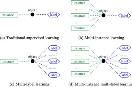
Fig. 1.Four different learning frameworks.

learning and generalized multi-instance learning is that in standard multi-instance learning there is a single concept, and a bag is positive if it has an instance satisfying this concept; while in generalized multi-instance learning [58,68] there are multiple concepts, and a bag is positive only when all concepts are satisfied (i.e., the bag contains instances from every concept). Recently, research on instance clustering [82], instance semi-supervised learning [49] and multi-instance active learning [60] have also been reported.

Multi-instance learning has also attracted the attention of theIlp_{community. It has been suggested that multi-instance} problems could be regarded as a bias on inductive logic programming, and the multi-instance paradigm could be the key between the propositional and relational representations, being more expressive than the former, and much easier to learn than the latter [23]. Alphonse and Matwin [1] approximated a relational learning problem by a multi-instance problem, fed the resulting data to feature selection techniques adapted from propositional representations, and then transformed the filtered data back to relational representation for a relational learner. Thus, the expressive power of relational representation and the ease of feature selection on propositional representation are gracefully combined. This work confirms that multi-instance learning can really act as a bridge between propositional and relational learning.

Multi-instance learning techniques have already been applied to diverse applications including image categorization [17, 18], image retrieval [71,84], text categorization [3,60], web mining [86], spam detection [37], computer security [54], face detection [66,76], computer-aided medical diagnosis [31], etc.

3. The MIML framework

Let

X

denote the instance space and

Y

the set of class labels. Then, formally, the MIML task is defined as:

•

MIML(multi-instance multi-label learning): To learn a function f

:

2X

→

2Y from a given data set

{

(

X1

,

Y1

), (

X2

,

Y2

),

. . . , (

Xm

,

Ym

)

}

, where Xi

⊆

X

is a set of instances

{

xi1

,

xi2

, . . . ,

xi,ni

}

, xi j

∈

X

(

j

=

1

,

2

, . . . ,

ni

)

, and Yi

⊆

Y

is a set of labels

{

yi1

,

yi2

, . . . ,

yi,li

}

, yik

∈

Y

(

k

=

1

,

2

, . . . ,

li

)

. Herenidenotes the number of instances in Xi andli the number of labels in Yi.

It is interesting to compare MIML with the existing frameworks of traditional supervised learning, multi-instance learning, and multi-label learning.

•

Traditional supervised learning(single-instance single-label learning): To learn a function f

:

X

→

Y

from a given data set

{

(

x1

,

y1

), (

x2

,

y2

), . . . , (

xm

,

ym

)

}

, wherexi

∈

X

is an instance and yi

∈

Y

is the known label ofxi.

•

Multi-instance learning (multi-instance single-label learning): To learn a function f

:

2X

→

Y

from a given data set

{

(

X1

,

y1

), (

X2

,

y2

), . . . , (

Xm

,

ym

)

}

, where Xi

⊆

X

is a set of instances

{

xi1

,

xi2

, . . . ,

xi,ni

}

, xi j

∈

X

(

j

=

1

,

2

, . . . ,

ni

)

, and

yi

∈

Y

is the label of Xi.2 Herenidenotes the number of instances in Xi.

•

Multi-label learning (single-instance multi-label learning): To learn a function f

:

X

→

2Y from a given data set

{

(

x1

,

Y1

), (

x2

,

Y2

), . . . , (

xm

,

Ym

)

}

, wherexi

∈

X

is an instance and Yi

⊆

Y

is a set of labels

{

yi1

,

yi2

, . . . ,

yi,li

}

, yik

∈

Y

(

k

=

1

,

2

, . . . ,

li

)

. Herelidenotes the number of labels inYi.

2 _{According to notions used in multi-instance learning,(X}

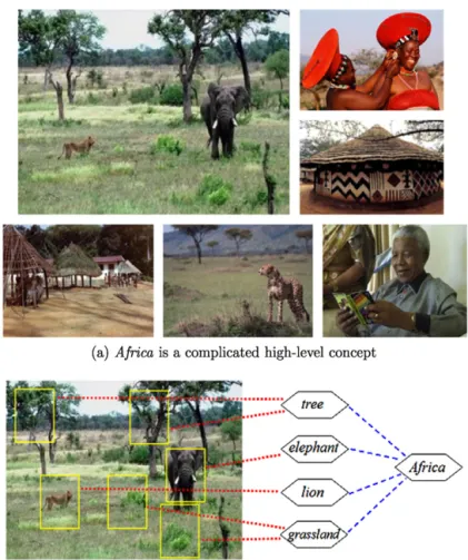
Fig. 2.MIML can be helpful in learning single-label examples involving complicated high-level concepts.

From Fig. 1 we can see the differences among these learning frameworks. In fact, the multi-learning frameworks are resulted from the ambiguities in representing real-world objects. Multi-instance learning studies the ambiguity in the input space (or instance space), where an object has many alternative input descriptions, i.e., instances; multi-label learning studies the ambiguity in the output space (or label space), where an object has many alternative output descriptions, i.e., labels; while MIML considers the ambiguities in both the input and output spaces simultaneously. In solving real-world problems, having a good representation is often more important than having a strong learning algorithm, because a good representation may capture more meaningful information and make the learning task easier to tackle. Since many real objects are inherited with input ambiguity as well as output ambiguity, MIML is more natural and convenient for tasks involving such objects.

It is worth mentioning that MIML is more reasonable than (single-instance) multi-label learning in many cases. Suppose a multi-label object is described by one instance but associated withlnumber of class labels, namely label1

,

label2

, . . . ,

labell. If we represent the multi-label object using a set ofninstances, namely instance1

,

instance2

, . . . ,

instancen, the underlying information in a single instance may become easier to exploit, and for each label the number of training instances can be significantly increased. So, transforming multi-label examples to MIML examples for learning may be beneficial in some tasks, which will be shown in Section 6. Moreover, when representing the multi-label object using a set of instances, the relation between the input patterns and the semantic meanings may become more easily discoverable. Note that in some cases, understanding why a particular object has a certain class label is even more important than simply making an accurate prediction, while MIML offers a possibility for this purpose. For example, under the MIML representation, we may discover that one object has label1 because it contains instancen; it has labell because it contains instancei; while the occurrence of both instance1 and instanceitriggers labelj.

MIML can also be helpful for learning single-label examples involving complicated high-level concepts. For example, as Fig. 2(a) shows, the conceptAfricahas a broad connotation and the images belonging toAfricahave great variance, thus it is not easy to classify the top-left image in Fig. 2(a) into theAfricaclass correctly. However, if we can exploit some low-level sub-concepts that are less ambiguous and easier to learn, such astree,lions,elephantandgrasslandshown in Fig. 2(b), it is possible to induce the conceptAfricamuch easier than learning the conceptAfricadirectly. The usefulness of MIML in this process will be shown in Section 7.

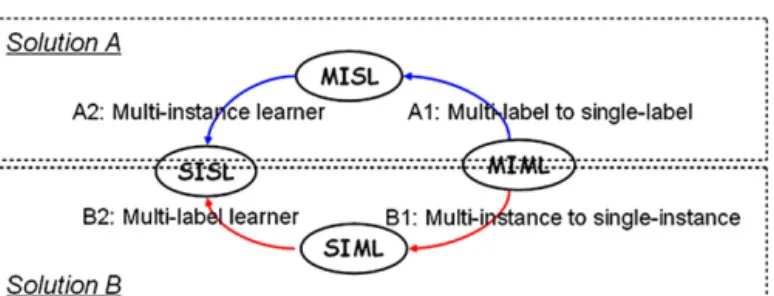
Fig. 3.The two general degeneration solutions.

4. Solving MIML problems by degeneration

It is evident that traditional supervised learning is a degenerated version of multi-instance learning as well as a degener-ated version of multi-label learning, while traditional supervised learning, multi-instance learning and multi-label learning are all degenerated versions of MIML. So, a simple idea to tackle MIML is to identify its equivalence in the traditional supervised learning framework, using multi-instance learning or multi-label learning as the bridge, as shown in Fig. 3.

•

Solution A: Using multi-instance learning as the bridge:

The MIML learning task, i.e., to learn a function f

:

2X

→

2Y, can be transformed into a multi-instance learning task, i.e., to learn a function fMIL

:

2X

×

Y

→ {−

1

,

+

1

}

. For any y

∈

Y

, fMIL

(

Xi

,

y

)

= +

1 if y

∈

Yi and

−

1 otherwise. The proper labels for a new example X∗ can be determined according to Y∗

= {

y

|

sign

[

fMIL

(

X∗

,

y

)

] = +

1

}

. This multi-instance learning task can be further transformed into a traditional supervised learning task, i.e., to learn a function

fSISL

:

X

×

Y

→ {−

1

,

+

1

}

, under a constraint specifying how to derive fMIL

(

Xi

,

y

)

from fSISL

(

xi j

,

y

) (

j

=

1

,

2

, . . . ,

ni

)

. For anyy

∈

Y

, fSISL

(

xi j

,

y

)

= +

1 ify

∈

Yiand

−

1 otherwise. Here the constraint can be fMIL

(

Xi

,

y

)

=

sign

[

n_ji₌₁fSISL

(

xi j

,

y

)

]

which has been used by Xu and Frank [70] in transforming multi-instance learning tasks into traditional supervised learning tasks. Note that other kinds of constraint can also be used here.

•

Solution B: Using multi-label learning as the bridge:

The MIML learning task, i.e., to learn a function f

:

2X

→

2Y, can be transformed into a multi-label learning task, i.e., to learn a function fMLL

:

Z

→

2Y. For any zi

∈

Z

, fMLL

(

zi

)

=

fMIML

(

Xi

)

ifzi

=

φ (

Xi

)

,

φ

:

2X

→

Z

. The proper labels for a new example X∗ can be determined according toY∗

=

fMLL

(φ (

X∗

))

. This multi-label learning task can be further transformed into a traditional supervised learning task, i.e., to learn a function fSISL

:

Z

×

Y

→ {−

1

,

+

1

}

. For any y

∈

Y

, fSISL

(

zi

,

y

)

= +

1 if y

∈

Yi and

−

1 otherwise. That is, fMLL

(

zi

)

= {

y

|

fSISL

(

zi

,

y

)

= +

1

}

. Here the mapping

φ

can be implemented withconstructive clustering which was proposed by Zhou and Zhang [93] in transforming multi-instance bags into traditional single-instances. Note that other kinds of mappings can also be used here.

In the rest of this section we will propose two MIML algorithms, MimlBoost andMimlSvm. MimlBoostis an illustration of Solution A, which uses category-wise decomposition for the A1 step in Fig. 3 andMiBoosting _{for A2;} MimlSvm_{is an} illustration of Solution B, which usesclustering-based representation transformationfor the B1 step andMlSvm_{for B2. Other} MIML algorithms can be developed by taking alternative options. BothMimlBoost _andMimlSvm_{are quite simple. We will} see that for dealing with complicated objects with multiple semantic meanings, good performance can be obtained under the MIML framework even by using such simple algorithms. This demonstrates that the MIML framework is very promising, and we expect better performance can be achieved in the future if researchers put forward more powerful MIML algorithms.

4.1. MimlBoost

Now we propose the MimlBoost algorithm according to the first solution mentioned above, that is, identifying the equivalence in the traditional supervised learning framework using multi-instance learning as the bridge. Note that this strategy can also be used to derive other kinds of MIML algorithms.

Given any set

Ω

, let

|

Ω

|

denote its size, i.e., the number of elements in

Ω

; given any predicate

π

, let

J

π

K

be 1 if

π

holds and 0 otherwise; given

(

Xi

,

Yi

)

, for any y

∈

Y

, let

Ψ (

Xi

,

y

)

= +

1 if y

∈

Yi and

−

1 otherwise, where

Ψ

is a function

Ψ

:

2X

×

Y

→ {−

1

,

+

1

}

which judges whether a label yis a proper label of Xior not. The basic assumption ofMimlBoost is that the labels are independent so that the MIML task can be decomposed into a series of multi-instance learning tasks to solve, by treating each label as a task. The pseudo-code ofMimlBoostis summarized in Appendix A (Table A.1).

In the first step of MimlBoost, each MIML example

₍

X_u

_,

Y_u

_{) (}

u

=

1

_,

2

_{, . . . ,}

m

₎

is transformed into a set of

|

Y

|

number of multi-instance bags, i.e.,

{[

(

Xu

,

y1

), Ψ (

Xu

,

y1

)

]

,

[

(

Xu

,

y2

), Ψ (

Xu

,

y2

)

]

, . . . ,

[

(

Xu

,

y|Y|

), Ψ (

Xu

,

y|Y|

)

]}

. Note that

[

(

Xu

,

yv

), Ψ (

Xu

,

yv

)

]

(

v

=

1

,

2

, . . . ,

|

Y

|

)

is a labeled multi-instance bag where

(

Xu

,

yv

)

is a bag containingnu number of instances, i.e.,

{

(

xu1

,

yv

), (

xu2

,

yv

), . . . , (

xu,nu

,

yv

)

}

, and

Ψ (

Xu

,

yv

)

∈ {−

1

,

+

1

}

is the label of this bag.

Thus, the original MIML data set is transformed into a multi-instance data set containingm

× |

Y

|

number of bags. We order them as

[

(

X1

,

y1

), Ψ (

X1

,

y1

)

]

, . . . ,

[

(

X1

,

y|Y|

), Ψ (

X1

,

y|Y|

)

]

,

[

(

X2

,

y1

), Ψ (

X2

,

y1

)

]

, . . . ,

[

(

Xm

,

y|Y|

), Ψ (

Xm

,

y|Y|

)

]

, and let

[

(

X(i)

_,

_y(i)

_{), Ψ (}

_X(i)

_,

_y(i)

₎

_]

_{denote thei-th of thesem}

_{× |}

_Y

_|

_{number of bags which containsn}

i number of instances. Then, from the data set a multi-instance learning function fMIL can be learned, which can accomplish the desired MIML function because fMIML

(

X∗

)

= {

y

|

sign

[

fMIL

(

X∗

,

y

)

] = +

1

}

. In this paper, the MiBoosting algorithm [70] is used to im-plement fMIL. Note that by using MiBoosting, the MimlBoost algorithm assumes that all instances in a bag contribute independently in an equal way to the label of that bag.

For convenience, let

(

B

,

g

)

denote the bag

[

(

X

,

y

), Ψ (

X

,

y

)

]

, B

∈

B

, g

∈

G

, and E denotes the expectation. Then, here the goal is to learn a function

F

(

B

)

minimizing the bag-level exponential loss E_BE_G|B

[

exp

(

−

g

F

(

B

))

]

, which ultimately estimates the bag-level log-odds function ₂1log_PrPr₍(_gg₌₋=1₁|B_|B)₎ on the training set. In each boosting round, the aim is to expand

F

(

B

)

into

F

(

B

)

+

c f

(

B

)

, i.e., adding a new weak classifier, so that the exponential loss is minimized. Assuming that all instances in a bag contribute equally and independently to the bag’s label, f

(

B

)

=

_n1

B

jh

(

bj

)

can be derived, where h

(

bj

)

∈ {−

1

,

+

1

}

is the prediction of the instance-level classifier h

(

·

)

for the j-th instance of the bag B, and nB is the number of instances inB.

It has been shown by [70] that the best f

(

B

)

to be added can be achieved by seeking h

(

·

)

which maximizes

i

ni j=1

[

1 niW (i)_g(i)_h

₍

_b(i)

j

)

]

, given the bag-level weights W

=

exp

(

−

g

F

(

B

))

. By assigning each instance the label of its bag and the corresponding weight W(i)

_/

_n

i, h

(

·

)

can be learned by minimizing the weighted instance-level classification error. This actually corresponds to the Step 3a ofMimlBoost_{. When f}

₍

_B

₎

_{is found, the best multiplierc}

_>

_{0 can be got by} directly optimizing the exponential loss:

E_BE_G|B

exp

−

g

F

(

B

)

+

c

−

g f

(

B

)

=

i W(i)exp

c

−

g (i)

jh

(b

(i) j

)

ni

=

i W(i)exp

2e(i)

−

1

c

,

(1) wheree(i)

₌

1 ni

j

J

(

h

(

b (i) j

)

=

g(

i)

₎

_K

_{(computed in Step 3b). Minimization of this expectation actually corresponds to Step 3d,}

where numeric optimization techniques such as quasi-Newton method can be used. Note that in Step 3c if e(i)

₀

_.

_{5, the}

Boosting process will stop [89]. Finally, the bag-level weights are updated in Step 3f according to the additive structure of

F

(

B

)

.

4.2. MimlSvm

Now we propose the MimlSvm_{algorithm according to the second solution mentioned before, that is, identifying the} equivalence in the traditional supervised learning framework using multi-label learning as the bridge. Note that this strategy can also be used to derive other kinds of MIML algorithms.

Again, given any set

Ω

, let

|

Ω

|

denote its size, i.e., the number of elements in

Ω

; given

(

Xi

,

Yi

)

and zi

=

φ (

Xi

)

where

φ

:

2X

→

Z

, for any y

∈

Y

, let

Φ(

zi

,

y

)

= +

1 if y

∈

Yi and

−

1 otherwise, where

Φ

is a function

Φ

:

Z

×

Y

→ {−

1

,

+

1

}

. The basic assumption ofMimlSvmis that the spatial distribution of the bags carries relevant information, and information helpful for label discrimination can be discovered by measuring the closeness between each bag and the representative bags identified through clustering. The pseudo-code ofMimlSvmis summarized in Appendix A (Table A.2).

In the first step ofMimlSvm, the X_u of each MIML example

₍

X_u

_,

Y_u

_{) (}

u

=

1

_,

2

_{, . . . ,}

m

₎

is collected and put into a data set

Γ

. Then, in the second step,k-medoids clustering is performed on

Γ

. Since each data item in

Γ

, i.e.Xu, is an unlabeled multi-instance bag instead of a single instance, Hausdorff distance [26] is employed to measure the distance. The Hausdorff distance is a famous metric for measuring the distance between two bags of points, which has often been used in computer vision tasks; other techniques that can measure the distance between bags of points, such as theset kernel[32], can also be used here. In detail, given two bags A

= {

a1

,

a2

, . . . ,

anA

}

andB

= {

b1

,

b2

, . . . ,

bnB

}

, the Hausdorff distance between A and

Bis defined as

dH

(

A

,

B

)

=

max

max

a∈Aminb∈B

a

−

b

,

maxb∈Bmina∈A

b

−

a

,

(2)

where

a

−

b

measures the distance between the instancesaandb, which takes the form of Euclidean distance here. After the clustering process, the data set

Γ

is divided into k partitions, whose medoids are Mt

(

t

=

1

,

2

, . . . ,

k

)

, re-spectively. With the help of these medoids, the original multi-instance example Xu is transformed into ak-dimensional numerical vectorzu, where thei-th

(

i

=

1

,

2

, . . . ,

k

)

component ofzuis the distance betweenXuandMi, that is,dH

(

Xu

,

Mi

)

. In other words, zui encodes some structure information of the data, that is, the relationship between Xu and the i-th partition of

Γ

. This process reassembles the constructive clustering process used by Zhou and Zhang [93] in transforming multi-instance examples into single-instance examples except that in [93] the clustering is executed at the instance level while here it is executed at the bag level. Thus, the original MIML examples

(

Xu

,

Yu

) (

u

=

1

,

2

, . . . ,

m

)

have been trans-formed into multi-label examples

(

zu

,

Yu

) (

u

=

1

,

2

, . . . ,

m

)

, which corresponds to the Step 3 ofMimlSvm.

Then, from the data set a multi-label learning function fMLL can be learned, which can accomplish the desired MIML function because fMIML

(

X∗

)

=

fMLL

(

z∗

)

. In this paper, the MlSvm algorithm [11] is used to implement f_MLL. Concretely, MlSvm decomposes the multi-label learning problem into multiple independent binary classification problems (one per class), where each example associated with the label set Y is regarded as a positive example when buildingSvm_{for any} class y

∈

Y, while regarded as a negative example when building Svm for any class y

∈

_/

Y, as shown in the Step 4 of MimlSvm. In making predictions, the T-Criterion[11] is used, which actually corresponds to the Step 5 of the MimlSvm algorithm. That is, the test example is labeled by all the class labels with positiveSvm_{scores, except that when all the}Svm scores are negative, the test example is labeled by the class label which is with thetop(least negative) score.

4.3. Experiments

4.3.1. Multi-label evaluation criteria

In traditional supervised learning where each object has only one class label,accuracyis often used as the performance evaluation criterion. Typically, accuracy is defined as the percentage of test examples that are correctly classified. When learning with complicated objects associated with multiple labels simultaneously, however, accuracy becomes less mean-ingful. For example, if approach Amissed one proper label while approach B missed four proper labels for a test example having five labels, it is obvious that A is better thanB, but the accuracy ofA andBmay be identical because both of them incorrectly classified the test example.

Five criteria are often used for evaluating the performance of learning with multi-label examples [56,92]; they are ham-ming loss,one-error,coverage,ranking lossandaverage precision. Using the same denotation as that in Sections 3 and 4, given a test set S

= {

(

X1

,

Y1

), (

X2

,

Y2

), . . . , (

Xp

,

Yp

)

}

, these five criteria are defined as below. Here,h

(

Xi

)

returns a set of proper labels of Xi;h

(

Xi

,

y

)

returns a real-value indicating the confidence for yto be a proper label of Xi;rankh

(

Xi

,

y

)

returns the rank of y derived fromh

(

Xi

,

y

)

.

•

hlossS

(

h

)

=

1p

p i=1

1

|Y|

|

h

(

Xi

)

Yi

|

, where

stands for the symmetric difference between two sets. Thehamming loss evaluates how many times an object-label pair is misclassified, i.e., a proper label is missed or a wrong label is pre-dicted. The performance is perfect when hlossS

(

h

)

=

0; the smaller the value of hlossS

(

h

)

, the better the performance ofh.

•

one-errorS

(

h

)

=

1_p

_ip₌₁

J

[

arg maxy∈Yh

(

Xi

,

y

)

]

∈

/

Yi

K

. The one-errorevaluates how many times the top-ranked label is not a proper label of the object. The performance is perfect when one-errorS

(

h

)

=

0; the smaller the value of one-errorS

(

h

)

, the better the performance ofh.

•

coverageS

(

h

)

=

1p

p

i=1maxy∈Yirank h

₍

_X

i

,

y

)

−

1. Thecoverageevaluates how far it is needed, on the average, to go down the list of labels in order to cover all the proper labels of the object. It is loosely related to precision at the level of perfect recall. The smaller the value of coverageS

(

h

)

, the better the performance ofh.

•

rlossS

(

h

)

=

1_p

_ip_=1|Yi||1_Yi|

|{

(

y1

,

y2

)

|

h

(

Xi

,

y1

)

h

(

Xi

,

y2

), (

y1

,

y2

)

∈

Yi

×

Yi

}|

, where Yi denotes the complementary set of Yi in

Y

. The ranking lossevaluates the average fraction of label pairs that are misordered for the object. The performance is perfect when rlossS

(

h

)

=

0; the smaller the value of rlossS

(

h

)

, the better the performance ofh.

•

avgprec_S

(

h

)

=

1_p

_ip_=1|Y1_i|

y∈Yi

|{y|rankh_(X

i,y)rankh(Xi,y), y∈Yi}| rankh(Xi,y)

. Theaverage precision evaluates the average fraction of proper labels ranked above a particular label y

∈

Yi. The performance is perfect when avgprecS

(

h

)

=

1; the larger the value of avgprecS

(

h

)

, the better the performance ofh.

In addition to the above criteria, we design two new multi-label criteria,average recallandaverage F1, as below.

•

avgrecl_S

(

h

)

=

1_p

_ip₌₁|{y|rankh(Xi,y)|h(Xi)|, y∈Yi}|

|Yi| . The average recallevaluates the average fraction of proper labels that have been predicted. The performance is perfect when avgreclS

(

h

)

=

1; the larger the value of avgreclS

(

h

)

, the better the performance ofh.

•

avgF1_S

(

h

)

=

2×avgprecS(h)×avgreclS(h)

avgprecS(h)+avgreclS(h) . The average F1expresses a tradeoff between theaverage precision and theaverage

recall. The performance is perfect when avgF1S

(

h

)

=

1; the larger the value of avgF1S

(

h

)

, the better the performance ofh.

Note that since the above criteria measure the performance from different aspects, it is difficult for one algorithm to outperform another on every one of these criteria.

In the following we study the performance of MIML algorithms on two tasks involving complicated objects with multiple semantic meanings. We will show that for such tasks, MIML is a good choice, and good performance can be achieved even by using simple MIML algorithms such asMimlBoostandMimlSvm.

4.3.2. Scene classification

The scene classification data set consists of 2000 natural scene images belonging to the classes desert, mountains,sea,

Table 1

Results (mean±std.) on scene classification data set (‘↓’ indicates ‘the smaller the better’; ‘↑’ indicates ‘the larger the better’). Compared

algorithms

Evaluation criteria

hloss↓ one-error↓ coverage↓ rloss↓ aveprec↑ averecl↑ aveF1↑

MimlBoost .193±.007 .347±.019 .984±.049 .178±.011 .779±.012 .433±.027 .556±.023

MimlSvm 189±.009 .354±.022 1.087±.047 .201±.011 .765±.013 .556±.020 .644±.018

MimlSvmmi .195±.008 .317±.018 1.068±.052 .197±.011 .783±.011 .587±.019 .671±.015

MimlNn .185±.008 .351±.026 1.057±.054 .196±.013 .771±.015 .509±.022 .613±.020

AdtBoost.MH .211±.006 .436±.019 1.223±.050 N/A .718±.012 N/A N/A

RankSvm .210±.024 .395±.075 1.161±.154 .221±.040 .746±.044 .529±.068 .620±.059

MlSvm .232±.004 .447±.023 1.217±.054 .233±.012 .712±.013 .073±.010 .132±.017

Ml-knn .191±.006 .370±.017 1.085±.048 .203±.010 .759±.011 .407±.026 .529±.023

as a bag of nine instances generated by theSbnmethod [46], which uses a Gaussian filter to smooth the image and then subsamples the image to an 8

×

8 matrix of color blobs where each blob is a 2

×

2 set of pixels within the matrix. An instance corresponds to the combination of a single blob with its four neighboring blobs (up, down, left, right), which is described with 15 features. The first three features represent the mean R, G, B values of the central blob and the remaining twelve features express the differences in mean color values between the central blob and other four neighboring blobs respectively.3

We evaluate the performance of the MIML algorithms MimlBoost _andMimlSvm_{. Note that}MimlBoost _andMimlSvm are merely proposed to illustrate the two general degeneration solutions to MIML problems shown in Fig. 3. We do not claim that they are the best algorithms that can be developed through the degeneration paths. There may exist other processes for transforming MIML examples into multi-instance single-label (MISL) examples or single-instance multi-label (SIML) examples. Even by using the same degeneration process as that used in MimlBoost andMimlSvm, there are also many alternatives to realize the second step. For example, by usingmi-Svm [3] to replace theMiBoostingused in Miml-Boostand by using the two-layer neural network structure [81] to replace theMlSvmused inMimlSvm, we getMimlSvm_mi andMimlNn_{respectively. Their performance is also evaluated in our experiments.}

We compare the MIML algorithms with several state-of-the-art algorithms for learning with multi-label examples, in-cludingAdtBoost.MH[22],RankSvm[27],MlSvm[11] andMl-knn[80]; these algorithms have been introduced briefly in Section 2. Note that these are single-instance algorithms that regard each image as a 135-dimensional feature vector, which is obtained by concatenating the nine instances in the direction from upper-left to right-bottom.

The parameter configurations ofRankSvm,MlSvm andMl-knnare set by considering the strategies adopted in [11,27] and [80] respectively. For RankSvm, polynomial kernel is used where polynomial degrees of 2 to 9 are considered as in [27] and chosen by hold-out tests on training sets. ForMlSvm, Gaussian kernel is used. ForMl-knn, the number of nearest neighbors considered is set to 10.

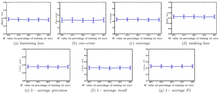
The boosting rounds of AdtBoost.MHandMimlBoost are set to 25 and 50, respectively; The performance of the two algorithms at different boosting rounds is shown in Appendix B (Fig. B.1), it can be observed that at those rounds the performance of the algorithms have become stable. Gaussian kernelLibsvm[16] is used for the Step 3a ofMimlBoost. The MimlSvm _andMimlSvm_{mi are also realized with Gaussian kernels. The parameter k of}MimlSvm _{is set to be 20% of the} number of training images; The performance of this algorithm with differentkvalues is shown in Appendix B (Fig. B.2), it can be observed that the setting ofk does not significantly affect the performance ofMimlSvm. Note that in Appendix B (Figs. B.1 and B.2) we plot 1 –average precision, 1 –average recalland 1 –average F1 such that in all the figures, the lower the curve, the better the performance.

Here in the experiments, 1500 images are used as training examples while the remaining 500 images are used for testing. Experiments are repeated for thirty runs by using random training/test partitions, and the average and standard deviation are summarized in Table 1,4where the best performance on each criterion has been highlighted in boldface.

Pairwise t-tests with 95% significance level disclose that all the MIML algorithms are significantly better than Adt-Boost.MHandMlSvm on all the seven evaluation criteria. This is impressive since as mentioned before, these evaluation criteria measure the learning performance from different aspects and one algorithm rarely outperforms another algorithm on all criteria. MimlSvm_andMimlSvm_{mi are both significantly better than}RankSvm _{on all the evaluation criteria, while} MimlBoostandMimlNnare both significantly better thanRankSvmon the first five criteria.MimlNnis significantly better than Ml-knnon all the evaluation criteria. Both MimlBoost and MimlSvm_mi are significantly better than Ml-knnon all criteria excepthamming loss.MimlSvmis significantly better thanMl-knnonone-error,average precision,average recall and average F1, while there are ties on the other criteria. Moreover, note that the best performance on all evaluation criteria are always attained by MIML algorithms. Overall, comparison on the scene classification task shows that the MIML algorithms can be significantly better than the non-MIML algorithms; this validates the powerfulness of the MIML framework.

3 _{The data set is available athttp://lamda.nju.edu.cn/data_MIMLimage.ashx.}

4 _{For the shared implementation ofAdtBoost.MH(http://www.grappa.univ-lille3.fr/grappa/en_index.php3?info=software),ranking loss,average recalland} average F1are not available in the program’s outputs.

Table 2

Results (mean±std.) on text categorization data set (‘↓’ indicates ‘the smaller the better’; ‘↑’ indicates ‘the larger the better’). Compared

algorithms

Evaluation criteria

hloss↓ one-error↓ coverage↓ rloss↓ aveprec↑ averecl↑ aveF1↑

MimlBoost .053±.004 .094±.014 .387±.037 .035±.005 .937±.008 .792±.010 .858±.008

MimlSvm .033±.003 .066±.011 .313±.035 .023±.004 .956±.006 .925±.010 .940±.008

MimlSvmmi .041±.004 .055±.009 .284±.030 .020±.003 .965±.005 .921±.012 .942±.007

MimlNn .038±.002 .080±.010 .320±.030 .025±.003 .950±.006 .834±.011 .888±.008

AdtBoost.MH .055±.005 .120±.017 .409±.047 N/A .926±.011 N/A N/A

RankSvm .120±.013 .196±.126 .695±.466 .085±.077 .868±.092 .411±.059 .556±.068

MlSvm .050±.003 .081±.011 .329±.029 .026±.003 .949±.006 .777±.016 .854±.011

Ml-knn .049±.003 .126±.012 .440±.035 .045±.004 .920±.007 .821±.021 .867±.013

4.3.3. Text categorization

The Reuters-21578 data set is used in this experiment. The seven most frequent categories are considered. After re-moving documents that do not have labels or main texts, and randomly rere-moving some documents that have only one label, a data set containing 2000 documents is obtained, where over 14.9% documents have multiple labels. Each document is represented as a bag of instances according to the method used in [3]. Briefly, the instances are obtained by splitting each document into passages using overlapping windows of maximal 50 words each. As a result, there are 2000 bags and the number of instances in each bag varies from 2 to 26 (3.6 on average). The instances are represented based on term frequency. The words with high frequencies are considered, excluding “function words” that have been removed from the vocabulary using theSmartstop-list [55]. It has been found that based on document frequency, the dimensionality of the data set can be reduced to 1–10% without loss of effectiveness [73]. Thus, we use the top 2% frequent words, and therefore each instance is a 243-dimensional feature vector.5

The parameter configurations ofRankSvm,MlSvmandMl-knnare set in the same way as in Section 4.3.2. The boosting rounds ofAdtBoost.MH andMimlBoost are set to 25 and 50, respectively. Linear kernels are used. The parameter k of MimlSvm_{is set to be 20% of the number of training images. The single-instance algorithms regard each document as a} 243-dimensional feature vector which is obtained by aggregating all the instances in the same bag; this is equivalent to represent the document using a sole term frequency feature vector.

Here in the experiments, 1500 documents are used as training examples while the remaining 500 documents are used for testing. Experiments are repeated for thirty runs by using random training/test partitions, and the average and standard deviation are summarized in Table 2, where the best performance on each criterion has been highlighted in boldface.

Pairwiset-tests with 95% significance level disclose that, impressively, bothMimlSvm_andMimlSvm_{mi are significantly} better than all the non-MIML algorithms. MimlNn is significantly better than AdtBoost.MH, RankSvm, and Ml-knn on all the evaluation criteria; significantly better than MlSvm onhamming loss,average recall andaverage F1while there are ties on the other criteria.MimlBoostis significantly better than AdtBoost.MHon all criteria except that there is a tie on hamming loss; significantly better than RankSvm_{on all criteria; significantly better than}MlSvm_{onaverage recalland there} is a tie onaverage F1; significantly better thanMl-knnonone-error,coverage,ranking loss andaverage precision. Moreover, note that the best performance on all evaluation criteria are always attained by MIML algorithms. Overall, comparison on the text categorization task shows that the MIML algorithms are better than the non-MIML algorithms; this validates the powerfulness of the MIML framework.

5. Solving MIML problems by regularization

The degeneration methods presented in Section 4 may lose information during the degeneration process, and thus a “direct” MIML algorithm is desirable. In this section we propose a regularization method for MIML. In contrast toMimlSvm andMimlSvm_{mi, this method is developed from the regularization framework directly and so we call it} D-MimlSvm_{. The} basic assumption of D-MimlSvm is that the labels associated to the same example have some relatedness, and the per-formance of classifying the bags depends on the loss between the labels and the predictions on the bags as well as on the constituent instances. Moreover, considering that for any class label the number of positive examples is smaller than that of negative examples, this method incorporates a mechanism to deal with class imbalance. We employ the constrained concave-convex procedure (Cccp) which has well-studied convergence properties [62] to solve the resultant non-convex optimization problem. We also present a cutting plane algorithm that finds the solution efficiently.

5.1. The loss function

Given a set of MIML training examples

{

(

X1

,

Y1

), (

X2

,

Y2

), . . . , (

Xm

,

Ym

)

}

, the goal of D-MimlSvm is to learn a map-ping f

:

2X

→

2Y where the proper label set for each bag X

⊆

X

corresponds to f

(

X

)

⊆

Y

. Specifically, D-MimlSvm

chooses to instantiate f with T functions, i.e. f

=

(

f1

,

f2

, . . . ,

fT

)

, where T is the number of labels in the label space

Y

= {

l1

,

l2

, . . . ,

lT

}

. Here, the t-th function ft

:

2X

→

R

determines the belongingness oflt for X, i.e. f

(

X

)

= {

lt

|

ft

(

X

) >

0

,

1

t

T

}

. In addition, each single instancex

∈

X

in a bag X can be viewed as a bag

{

x

}

containing only one instance, such that f

(

{

x

}

)

=

(

f1

(

{

x

}

),

f2

(

{

x

}

), . . . ,

fT

(

{

x

}

))

is also a well-defined function. For convenience, f

(

{

x

}

)

and ft

(

{

x

}

)

are simplified as f

(

x

)

and ft

(

x

)

in the rest of this section.

To train the component functions ft

(

1

t

T

)

in f, D-MimlSvm _{employs the following empirical loss function V} involving two terms (balanced by

λ

):

V

{

Xi}m_i=1

,

{

Yi}m_i=1

,

f

=

V1

{

Xi}m_i=1

,

{

Yi}m_i=1

,

f

+

λ

·

V2

{

Xi}m_i=1

,

f

.

(3)

Here, the first termV1 considers the loss between the ground-truth label set of each training bagXi, i.e.Yi, to its predicted label set, i.e. f

(

Xi

)

. Letyit

=

1 iflt

∈

Yiholds (1

i

m

,

1

t

T). Otherwise,yit

= −

1. Furthermore, let

(

z

)

+

=

max

(

0

,

z

)

denote the hinge loss function. Accordingly, the first loss termV1is defined as:

V1

{

Xi}m_i=1

,

{

Yi}m_i=1

,

f

=

1 mT m

i=1 T

t=1

1

−

yitft

(

Xi

)

+

.

(4)

The second termV2 considers the loss between f

(

Xi

)

and the predictions ofXi’s constituent instances, i.e.

{

f

(

xi j

)

|

1

j

ni

}

, which reflects the relationships between the bag Xiand its instances

{

xi1

,

xi2

, . . . ,

xi,ni

}

. Here, the common assumption in multi-instance learning is that the strength for Xi to hold a label is equal to the maximum strength for its instances to hold the label, i.e. ft

(

Xi

)

=

maxj=1,...,ni ft

(

xi j

)

.

6 _{Accordingly, the second loss termV}

2 is defined as: V2

{

Xi}m_i=1

,

f

=

1 mT m

i=1 T

t=1 l

ft

(

Xi

),

max j=1,...,ni ft

(x

i j

)

.

(5)

Here,l

(

v1

,

v2

)

can be defined in various ways and is set to be thel1loss in this paper, i.e.l

(

v1

,

v2

)

= |

v1

−

v2

|

. By combining Eq. (4) and Eq. (5), the empirical loss functionV in Eq. (3) is then specified as:

V

{

Xi}m_i=1

,

{

Yi}m_i=1

,

f

=

1 mT m

i=1 T

t=1

1

−

yitft

(

Xi

)

+

+

λ

mT m

i=1 T

t=1 l

ft

(

Xi

),

max j=1,...,ni ft

(x

i j

)

.

(6)

5.2. Representer theorem for MIML

For simplicity, we assume that each function ft is a linear model, i.e., ft

(

x

)

=

wt

, φ (

x

)

where

φ

is the feature map induced by a kernel functionkand

·

,

·

denotes the standard inner product in the Reproducing Kernel Hilbert Space (RKHS)

H

induced by the kernelk. We recall that an instance can be regarded as a bag containing only one instance, so the kernel

kcan be any kernel defined on a set of instances, such as the set kernel[32]. In the case of classification, objects (bags or instances) are classified according to the sign of ft.

D-MimlSvmassumes that the labels associated with a bag should have some relatedness; otherwise they should not be associated with the bag simultaneously. To reflect this basic assumption,D-MimlSvmregularizes the empirical loss function in Eq. (6) with an additional term

Ω(

f

)

:

Ω(

f

)

+

γ

·

V

{

Xi}m_i=1

,

{

Yi}m_i=1

,

f

.

(7) Here,

γ

is a regularization parameter balancing the model complexity

Ω(

f

)

and the empirical riskV. Inspired by [28], we assume that the relatedness among the labels can be measured by the mean functionw0,

w0

=

1 T T

t=1 wt

.

(8)

The original idea in [28] is to minimize

_tT₌₁

wt

−

w0

2 and meanwhile minimize

w0

2, i.e. to set the regularizer as:

Ω(

f

)

=

1 T T

t=1

wt

−

w0

2

+

η

w0

2

.

(9)

6 _{Note that this assumption may be restrictive to some extent. There are many cases where the label of the bag does not rely on the instance} with the maximum predictions, as discussed in Section 2. In addition, in classification only the sign of prediction is important [19], i.e.sign(ft(Xi))= sign(maxj=1,...,nift(xi j)). However, in this paper the above common assumption is still adopted due to its popularity and simplicity.