Hierarchical regression learning for car pose estimation

Dan Yang

University of Tampere

School of Information Sciences M.Sc. Thesis

Supervisors: Dr. Ke Chen Dr. Eleni Berki

University of Tampere

School of Information Sciences Major: Software Development

DAN YANG: Hierarchical Regression Learning for Car Pose Estimation M.Sc. Thesis, 46 pages

December 2016

Keywords: pose estimation, visual regression, hierarchical framework, target coding, pose-sensitive parts, coarse classifiers, fine regressors, method evaluation.

Finally, I finished this thesis work in my fourth winter in Finland. I would like to express my gratitude to all the people who have helped me during the passed whole year.

Foremost, I want to thank my supervisors, Dr. Ke Chen (Tampere University of Tech-nology), Dr. Eleni Berki (University of Tampere) and Prof. Joni-Kristian Kämäräinen (Tampere University of Technology), for all their support and help. I really admire the intelligence of Dr. Chen in research work. He always gave me great ideas and patient guidance which encouraged me to complete this thesis. My special thanks go to Eleni, for her unfailing support during my study. I really appreciate her valuable comments and advice for writing a high-quality thesis. I felt deeply indebted to Prof. Kämäräinen for his insightful advice and providing me the opportunity to work on such an interesting topic.

I would like to express my gratitude to my lovely colleagues, Yanlin Qian and Dingding Cai. Efficient discussion and cooperation with them helped me in achieving better results. I also want to thank all the members work in Computer Vision Group of Tampere Univer-sity of Technology who have supported in my study. I feel very lucky working in such an inspiring and productive group.

Many thanks go to my friend Gaoming Zheng who is always supportive when I have difficulties. Finally, I would like to express my special thanks to my family, especially my parents, whose unconditional love is the biggest motivation for me to continue study in Finland.

Tampere, December 15th, 2016

CONTENTS

1 INTRODUCTION 3

1.1 Motivation . . . 3

1.2 Objectives . . . 4

1.3 Research Methodologies . . . 5

1.4 Structure of the Thesis . . . 7

2 BACKGROUND 8 2.1 Car Pose Estimation . . . 8

2.2 Challenges . . . 10 2.3 State-Of-The-Art Algorithms . . . 12 2.4 Public Benchmarks . . . 14 2.5 Summary . . . 16 3 Regression Methods 17 3.1 Regression Forests . . . 17

3.2 K-clustering Regression Forest . . . 19

3.3 Experimental Verification . . . 20

3.4 Summary . . . 21

4 Part-Aware Target Coding 22 4.1 Introduction . . . 22

4.2 Pipeline . . . 25

4.3 Visible Semantic Parts . . . 26

4.4 Part-Aware Target Coding . . . 26

4.5 Regression Mapping onto Viewpoint Space . . . 27

4.6 Experiments . . . 28

4.7 Summary . . . 30

5 Hierarchical Sliding Slice Regression 32 5.1 Introduction . . . 32

5.2 Pipeline . . . 35

5.3 Circular Slice Construction . . . 35

5.4 Coarse Classifier . . . 36

5.5 Fine Slice-Specific Regressor . . . 37

5.6 Experiments . . . 38

5.7 Summary . . . 41

List of Figures

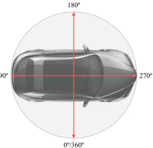
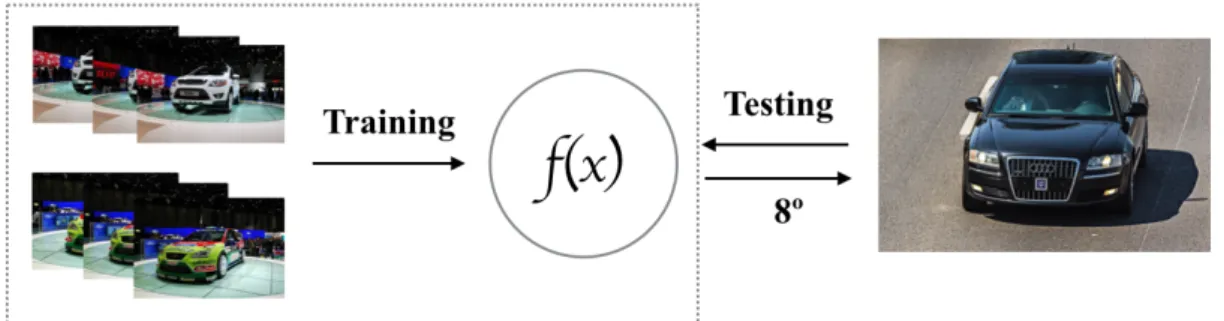
1.1 The car pose should be estimated as the front direction (270o_{) in the} cir-cular output space. . . 4 2.1 Abstract pipeline for pose estimation problem: (1) in the training stage,

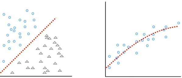
features of training data set with ground-truth are used to train a predictive model; (2) The model is used to predict the viewing angle of a unknown testing image. . . 8 2.2 Classification vs Regression . . . 9 2.3 Illustrative examples of the problem specific characteristics of

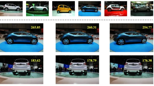
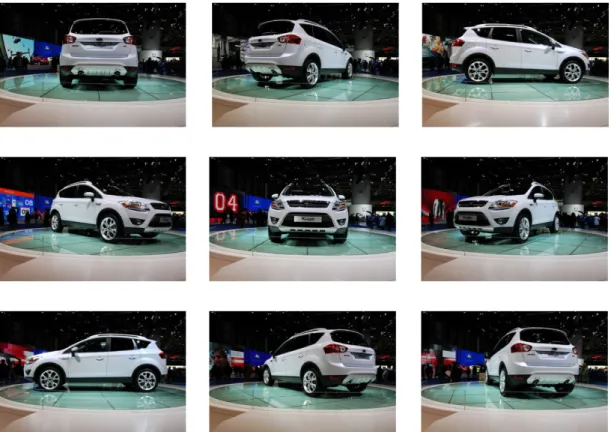
vision-based car pose estimation. Top: visual differences between different mod-els for the same viewing angle; middle: visual similarity of the neighbour-ing viewneighbour-ing angles for the same car; bottom: problem-specific circular similarity of flipping pose. . . 11 2.4 Examples from the EPFL Multi-view Car Dataset. . . 15 3.1 Using standard binary splitting rules to construct a regression tree:

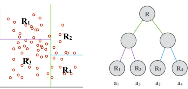
se-lect a splitting rule from pre-defined set of splitting rule that minimise SSE and then forward training samples into two child nodes according to the selected rule. If stopping criterion is reached then stop splitting. As shown in the left of the figure the input space is first divided into two partitions by the certain splitting rule (green line) and each partition is divided by different rules respectively. Finally the whole input space is divided into4partitions (K = 4). The tree structure is shown in the right side. The output of each leaf can be represented as ai = _n1

i

P

xi∈Riyi

withni denoting the number of training samples that are forwarded into the input subspaceRi. . . 18 3.2 Three steps of K-clusters splitting method (K = 3) for regression tree

construction: (1) Cluster the training data into 3 groups by applying K-means on the target space (left). (2) Divide the input space into 3 sub-spaces by SVM which can preserve the found clusters as much as pos-sible (middle) and forward training samples into three child nodes. (3) A constant estimate is calculated for each subspace if no more partition-ing is needed. Some misclassification is unavoidable shown as some data points that changed color (right). . . 20 4.1 A sequence of images from EPFL Multi-View Car benchmarks. Each

image is highlighted by semantic visible parts. . . 23 4.2 Working flow of the proposed framework. . . 24

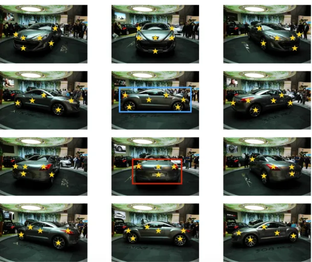
4.3 16 parts were manually labelled for all the image in dataset and SVM classifiers were trained independently for 16 parts of car: (1) front license number; (2) back license number; (3) front logo; (5) front left light; (6) front right light; (7) back left light; (8) back right light; (9) front left wheel; (10) front right wheel; (11) back left wheel; (12) back right wheel; (13) left mirror; (14) right mirror; (15) left door(s); (16) right door(s). When the HOG feature is feed to the classifiers probabilities of the 16 parts will be predicted. As shown in the right side, there are 5 parts are predicted to be highly probable with higher than0.95for the parts labelled with red numbers: (10) front right wheel, (12) back right wheel and (14) right mirror. . . 25 4.4 Comparison of PAR (ours), KRF and AKRF on mae (100%) for each

sequence (leave-one-sequence-out). . . 30 4.5 The top row shows the cars in sequences 7, 9 and 10 on which our

meth-ods reducing mae . . . 31 5.1 Intuitive concept of the proposed HSSR. . . 33 5.2 Our approach for estimating car pose hierarchically by first coarse

group-ing via classification and then fine estimation via regression. . . 34 5.3 Comparison of HSSR (ours), KRF and AKRF on mae (100%) for each

sequence (leave-one-sequence-out). . . 40 5.4 Comparative cumulative scores. The higher the better. . . 41

List of Tables

3.1 Evaluation of the KRF and AKRF with the EPFL Multi-View Car dataset. 20 4.1 Comparative evaluation of the state-of-the-art methods with the EPFL

Multi-View Car dataset. . . 29 5.1 Comparative evaluation of the state-of-the-art methods with the EPFL

Multi-View Car dataset. . . 39 5.2 Evaluation on the circular slice step size proportional to the45◦slice size. 40 5.3 Evaluation on the circular slice size. . . 40

ABSTRACT

Car pose estimation is a hot topic in computer vision because of its significance in intel-ligent transportation system. Considering the circular label space of car pose, the main limitation of classification approach is that the natural latent continuous-changing corre-lation across pose labels are omitted. It is more meaningful to formulate this problem as a continuous regression problem. However, the changing of light conditions and various vehicle models make imagery feature very inconsistent which easily leads global regres-sion methods fail. In order to improve the robustness of regresregres-sion learning, we proposed two novel hierarchical frameworks both of which consist of weak classifiers and strong regressors. In the first framework, Part-Aware Target Coding (PATC), the classifiers are used to predict probabilities of presence of some visible pose-sensitive parts. The proba-bilities together with the low level imagery features can be used as more consistent input features to train a strong regressor. The second framework, Hierarchical Sliding Slice Regression (HSSR), is in a coarse-to-fine manner. Coarse classifiers are first used to determine the belonging target group and the target group optimised fine regressors are used to estimate viewing angles. These two frameworks are applied on the benchmarking EPFL Multi-view car dataset and both of them achieve superior performance as compared to the state-of-the-art approaches.

ABBREVIATIONS AND SYMBOLS

RF Regression Forests

KRF K-clustering Regression Forests

AKRF Adaptive K-clustering Regression Forests PAR Parts-Aware Regression

HSSR Hierarchical Sliding Slice Regression SVM Support Vector Machine

RBF Radial Basic Function MAP Maximum a Posterior SSE Sum of Square Errors

BIC Bayesian Information Criterion MAE Mean Absolute Errors

HOG Histogram Oriented Gradients RBM Restricted Boltzmann Machines

1

INTRODUCTION

1.1

Motivation

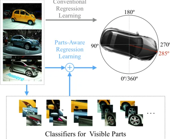
Pose estimation, which attempts to predict the viewing angle of a target object in a given image, is a hot topic in the field of computer vision. Target objects can be still lives, liv-ing beliv-ings and body parts [1, 2, 3, 4, 5]. Different objects have different characteristics due to the specific nature of the objects. Therefore, pose estimating methods are usually specifically formulated for the target object. Pose estimation can be considered as a classi-fication problem if the label space is viewed as a set of discrete integers, or as a regression problem if the continuous output is pursued. This thesis aims to solve the pose estimation problem of vehicle. As shown in Figure 1.1, the pose (known as ’viewing angles’) of a car normally indicates the front direction which can be described as a horizontal rotation. Car pose is changing in a continuous and cumulative way (from0o_to360o_{). Considering} of the circular label space, car pose estimation should be inherently a regression problem.

Car pose estimation has its significance in intelligent transportation systems. It is closely related with autonomous driving systems since the viewing angles of surrounding ve-hicles of an autonomous driving car imply its possible past and future paths. Typical onboard sensors such as radars or laser range finders work effectively in measuring inter-vehicle distance, while visual sensors in terms of onboard front, side and back cameras, provide rich imagery information for viewpoint estimation. A number of applications utilising estimated vehicle viewpoint have been proposed in the field of intelligent trans-portation [6, 7, 8, 9, 10, 11]. Generally, this problem is solved by training a mapping function mapping from input space to target space. However, large variation of the low-level input imagery feature usually makes the mapping challenging.

Car pose estimation problem has been discussed in the literature in recent few years. It is originally cast as a classification problem [12], where the360o_{pose space is quantised} into a number of bins and a multi-class classifier is trained to learn the mapping from imagery feature space to the discrete angle range classes. However, the main limitation of the classification approach is that the class labels are explicitly made independent which omits the natural latent continuously-changing correlation across pose class labels. For example, the closer the pose class labels of a pair of images are, the more visually similar these two images are. Therefore, learning of the classes benefits from examples in both classes. In the light of this, it is more meaningful to cast car pose estimation as a regression problem [13, 14, 4]. In visual regression, the goal is to learn a mapping from the imagery

Figure 1.1. The car pose should be estimated as the front direction (270o) in the circular output space.

feature space to a continuous real-valued target space. The existing regression methods for vehicle viewpoint direction incorporate manifold locality into either explicit feature representation [13, 14] or implicit regression model training [4]. However, these methods omitted the special characteristics of the problem due to the repetitive visual structure of the vehicles and the circular output space.

1.2

Objectives

The imaging distortion, such as illumination and perspective changes, makes the regres-sion approaches mapping from the imagery feature space to the label space challenging. Many methods have been proposed to solve the inconsistent input-output relationship in regression learning in recent years. In this thesis state-of-the-art regression methods are reviewed in order to understand the background of car pose estimation. Among these methods, K-clustering Regression Forests (KRF) framework proposed by Kotaet al. [4] has shown good efficiency in solving pose estimation problems and achieved

state-of-the-art performance. The theoretical principles behind KRF will be explored, and the advancement of KRF will be verified by experiments in Section 3. The goal of this thesis is to formulate more robust regression frameworks for car pose estimation and beat the performance of KRF. The following research questions are tackled and answered in this thesis:

1 What are the specific characteristics for car pose estimation problem?

2 How can the performance of regression framework be improved by utilising these characteristics?

The pose estimation problem this thesis aims to solve is specific for car. In order to answer the first question, observation of related datasets is necessary. The samples in EPFL Multi-view car dataset that are collected from an auto show contain 20 sequences of different types of cars rotating in various directions. Inspired by the characteristics of this dataset and previous works, ideas can be generated to boost the performance for car pose estimation.

1.3

Research Methodologies

The topic area is identified as car pose estimation and the research questions are tractable which make the goal of this thesis clear – specifying the characteristics of car pose es-timation and utilising these characteristics to formulate novel frameworks to boost the estimating performance. Performance is represented by how accuracy the frameworks can predict the viewing angles of testing dataset. Recorded results from experiments ev-idently indicate whether the proposed frameworks are successful by comparing with the state-of-the-art. The following list of methodologies are used to conduct the research in this thesis:

Literature Review –The goal of literature review in this thesis is to provide comprehen-sive background information about the topic and the significance of the state-of-the-art approaches [15]. Pose estimation has been studied in the literature for decades. New methods have been proposed to beat the performance of previous works. Therefore, the main literature in this thesis includes the papers which achieved considerable results for car pose estimation in recent years. New ideas can be inspired by identifying the failed ex-amples in previous research. Besides, related works bring effective experimental methods

which can be used to verify the novel methods proposed in this thesis. These literatures are mostly selected from publications of top journals and conferences in computer vision.

Model Methodology – Given the input data and the corresponding labels, reflecting on how to construct a better mapping function is the most important research work in this thesis. Ideas can be inspired by reviewing related works or observing dataset. Models are abstraction of the mature ideas, which can also be used as instruments to study and under-stand the research object [16]. This thesis aims to formulate robust regression methods for car pose estimation. The input sample is imagery feature extracted from the EPFL dataset and the corresponding labels are the manually-annotated viewing angles. Two proposed novel frameworks are all in a hierarchical fashion. How these frameworks are constructed from the first layer of weak classifiers and the second layer of strong regressors are spec-ified and visualised as diagrams in Section 4 and 5 respectively.

Formal Methodology – Formal methods are the foundation to describe the proposed methods that allows for general results which can be used as underlying technologies in solving other similar problems [16]. The essence of the contribution of this thesis work is abstracted into concise description with standardised syntax. The Input-Output is clearly defined and the operations are precisely expressed in mathematical language. Researchers can easily check if the model is implementable to address certain problem by reading the formal specification.

Experimental Methodology – Experiments are widely used to evaluate new methods for problems in empirical research. Better results from experiments evidently explain why the proposed methods are superior by comparing with the performance of previous approaches. Experimental verification is also the best way to explore deeply with the new methods to discover limitations or potential that can be used to boost the performance. In order to conduct the experiments in a justifiable and sufficient way, identical settings of the previous works are adopted, the data-split setting for instance, and all the free parameters are chosen by cross-validation. Multiple groups of experiments need to be designed to evaluate the proposed methods from different aspects, especially when novel concepts are introduced. A large number of results are generated during the experiments. It is important to only present the results that are germane to the research questions, otherwise tedious report may confuse the point of this thesis work. The results should be stated clearly in plain language. Tables and graphs are indispensable to visualise the statistics. The discussion includes the explanation of the presented results and the insight of them – the gained knowledge [16].

The listed methodologies are employed to tackle the research questions. Each of them plays an important role in different stage of the study. Literature review and model methodologies are utilised as instruments to study and understand the the research objects. The proposed frameworks are described in formal specification that allows autonomous verification. Well-designed experiments evaluate these approaches whether they have achieved the objects.

1.4

Structure of the Thesis

The rest of the thesis is organised as follows. In Section 2, theoretical background of car pose estimation problem is introduced in details. First of all, a clear definition of this problem is given and how the two general approaches, classification and regression, handle with this problem is briefly explained. Then current challenges and literatures of related works are discussed. Finally, there is the introduction to the benchmarking EPFL Multi-view car dataset. Section 3 is an deep exploration to our baseline method K-clustering Regression Forests. The theoretical detail is investigated and the performance is experimentally verified. The two main contributions of this thesis, Part-Aware Target Coding framework and Hierarchical Sliding Slice Regression framework, are introduced in Section 4 and Section 5 respectively. Both frameworks are evaluated on the benchmark-ing dataset. Final conclusion of the thesis work and future lines of research are shown in Section 6.

2

BACKGROUND

2.1

Car Pose Estimation

Car pose estimation is aimed at training a model to predict the front direction of an un-known car. It plays an important role in intelligent transportation system, such as vehicle recognition and tracking, but is difficult to perform with typical onboard sensors such as radars and laser rangefinders which work effectively in obstacles distance estimating. The model is required to be robust and accurate in real-time applications in the field of intel-ligent transportation and visual surveillance. Combining both in-vehicle sensor data and visual information [6] can be an reliable approach to estimate the viewing angles . Recent development of onboard car camera systems which provide rich information about the surrounding cars and the background enable vision based car pose estimation [7].

In computer vision, pose estimation is a hot but challenging topic. Generally, the esti-mating approach is to train a mapping model from feature space onto a target space. The label of an unknown image can be predicted by the trained model. The abstract pipeline for training such a model for car pose estimation is illustrated in Figure 2.1. Features that extracted from training image dataset are first used to train a mapping function between the input space and the label space. Then the model can be applied for predicting the viewing angle of a test image. Pose estimation methods are specified for different object according to the characteristics of objects,e.g. human head pose estimation includes hor-izontal direction and vertical direction and for each direction head pose can only change in a limited range, but for a car, the situation is different. The label space for a car is a cyclic.

Figure 2.1. Abstract pipeline for pose estimation problem: (1) in the training stage, features of

training data set with ground-truth are used to train a predictive model; (2) The model is used to predict the viewing angle of a unknown testing image.

Most of the car pose estimating approaches proposed so far can be split into two types of frameworks: regression-based approaches [13, 14, 4] and classification-based approaches [12, 17]. Considering of that the viewing angle of a car is changing in a continuous and cumulative way, car pose estimation can be regarded as a regression problem in this thesis. The principles behind both classification and regression approaches are briefly introduced in the follow. The training data is denoted as{xi, yi}N, i = 1,2, . . . , N,x ∈Rp, y ∈ R wherexi is the representation of imagery feature of a car in the training dataset, andyi is the labeled pose.

Classification –When pose labels are considered as discrete classes, the pose estimation is a classification problem[18]. The task of classification is to find the boundaries that can separate data into groups. Among the classification methods, Support Vector Machine performs effectively in leaning an optimal separating hyperplanewx+b = 0that max-imises the margin between different groups of data [18]. Intuitive concept is illustrated in the left side of Figure 2.2 that the classification is optimised by finding the discriminative boundary (red line) to which the closest data point has the maximum distance.

Regression –In regression frameworks, the labels are changing in a continuous manner. The basic idea of regression is learning a functionf(x)that has befitting deviation from the actual targetyi for the training dataxi [18]. The right side of Figure 2.2 shows the regression function which is to fit the training data points by minimising the the distance betweenf(xi)and the target valueyi.

A comparison work between classification and regression has been done by Guo et al. [18]. They experimentally verifying these two methods on head pose estimation (in-cludes horizontal and vertical directions). The results show that classification method performs better than regression in vertical pose estimation but much worse in horizontal pose estimation. Because the distributions of the face patterns have large overlapping in the horizontal directions but less serious in the vertical direction [18]. For car pose esti-mation, the pose clearly means the frontal direction changing in a horizontal circular. The poses of a car in similar viewing angles have subtle visual differences which indicates a relation of dependency between two neighbouring labels. In the light of this, car pose estimation is inherently a regression problem.

2.2

Challenges

Given visual observations from images or video frames and corresponding vehicle view-points as input and output respectively, a regression function is trained and then applied for estimating poses in test images. It is challenging to learn such a mapping relation between high-dimension imagery features and low-dimension pose labels. Successful regression function strongly relies on good feeding features; however in computer vi-sion, the training images are considered ill-suited for directly estimating pose [2]. As mentioned in Section 2.1 that classification approaches omit the dependency between neighbouring labels, but the inconsistency of training data always lead a global regression model lack the quality to represent label variation. The imagery feature inconsistency can be caused by different light conditions, image distortion, or noisy in background. The sit-uation for car pose estimation is even more complicated due to the real-time applications are usually in a changing environment which is full of noisy factors. The model needs to be robust enough to handle with images taken under such a condition. Except the com-putational complexity and the inconsistent features, there are many challenges caused by the specific characteristics of cars, sparsity of data and ambiguity of labels [5].

Figure 2.3. Illustrative examples of the problem specific characteristics of vision-based car pose estimation. Top: visual differences between different models for the same viewing angle; middle: visual similarity of the neighbouring viewing angles for the same car; bottom: problem-specific circular similarity of flipping pose.

On one hand, both visual variation and similarity can make car pose estimation challeng-ing. As shown in the top row in Figure 2.3, the visual dissimilarity between different car types can be significant. The illustrated cars have different colours and outlines, and some of them are designed in very uniquely fashionable shapes. The difference of appearance increase the inconsistency of input features. However, visual differences between similar viewing angles can be subtle (see the middle two rows of Figure 2.3). A global regression model may be inadequate to represent the changes of labels by giving such similar inputs. Moreover, there is axial symmetry in similarity which easily leads estimation subject to 180o _{flipping errors, e.g. between the front and back views and the left and right side} views (shown in the bottom row of Figure 2.3) which represents the maximal difference in the output space (−180◦vs+180◦).

On the other hand, collecting data for training model is a labourious task. EPFL multi-view car data set contains only 20 image sequences of different car models taken from an auto show and then the data are further splitted into two sets for training and testing which easily leads the training data more sparse. Moreover, the annotated labels are calculated by using time stamp assuming that all images are taken under a constant velocity, which affects the ground-truth, e.g. there are many neighbouring images of the same car that have the same time stamp but the viewing angles slightly vary with each other [13]. As a result, the images with the same label have different poses.

2.3

State-Of-The-Art Algorithms

A number of methods have been proposed to address the in inconsistent feature-pose relation. This subsection mainly reviews preview works that have achieved state-of-the-art performance on car pose estimation [12, 13, 14, 4]. Car pose estimation was originally cast as a classification problem [12], which quantized circular label space into a number of pose bins and a SVM classifier is trained for each discrete pose. Support Vector Machine (SVM) [19] is a widely used algorithm the good performance it has achieved in dealing with classification problems. The standard SVM is utilised in two-classes classification problem. For a multi-class problem, such as 16 pose bins in car pose estimation, it is general to learn a classifier for each class against all the rest classes (one-vs-all). SVM performs effectively in finding margins to divide discrete classes with largest distance between them, but when the labels are continuously changing it may give poor results as proved in [18]. If the continuous label space is divided into discrete quantised pose classes, the latent correlation across pose class labels is omitted. For example, the closer pose class labels of a pair of images are, the more visual similarity these two images

share with. Increasing the number of class labels may create more precise estimation but at the same time makes the classification problem more computational complex [4]. K-means clustering which automatically separates the label space can solve the classification problem by using induction algorithms, but still the label space is discrete.

There are many regression methods have been proposed in order to solve this problem. In [13], before regression mapping an embedded representation of the local features and their spacial arrangement are learned and then enforce supervised manifold constraints in the embedding to achieve smooth image similarity changing. The final regression map-ping from the data point on the learned manifold to the target label space is trained by using Radial Basic Function (RBF). Instead of applying regression to whole images as atomic units, Fenzi [14] formulated a set of local feature generative models to separately represent individual parts appearing on a instance. The pose is estimated using maximum a posteriori (MAP) inference. Foytic [2] acknowledged that methods globally modelling with linear function are too challenging, and they proposed a region-dependent regression framework. Given a testing image, the range of the predicted label is first approximately determined and then the real label is calculated by using a local-specific regression func-tion. Among some non-linear regression approaches, regression forests has achieve good performance in pose estimation problems. Based on standard regression forests, Hara [4] proposed K-clustering Regression Forests (KRF) by introducing a more flexible node splitting algorithm. In the splitting stage, training samples are clustered into K clusters according to the distribution of the label space and then a SVM classifier is trained for each of these clusters to distinguish each other. Finally data is splitted into K child nodes by using these classifiers. KRF achieves good performance in pose estimation problem because the novel splitting algorithm has more freedom in choosing partitioning rule than the binary splitting.

As discussed before, the car pose estimation is considered as a regression problem. The regression methods that are reviewed in this subsection explored different ways to im-prove accuracy for pose estimation. The challenges discussed in 2.2 limit the performance of regression approaches for direct pose estimation. In order to overcome the inconsistent input-output relation of global regression frameworks, hierarchical regression frameworks are more robust in representing the changing of label pose by dividing the regression pro-cess into layers. The problem-specific characteristics of cars can be utilised in designing such frameworks from two aspects:

1 The variation of appearances of different car models influences the quality of the input features. However, there is a group of visible parts which consistently exist

in different car models, such as wheels, lights and license boards, can be utilised to equip the input features. Manually labeling these parts for each image in the dataset is necessary since in this way classifiers to predict the presence of these parts can be trained. The prior information is middle level features that can be combined with low-level imagery features in regressor training.

2 Inspired by the hierarchical regression framework [2], the circular label space can be divided into several subspaces. A regressor is trained for each subspace. A testing image is first coarsely classified into a subspace and the local-specific fine regressor is used to predict the viewing angles. In such a coarse-to-fine fashion, challenges of global regression can be avoided since each fine regressor can ade-quately estimate the continuously changing angles .

Classification approach performs effectively in solving estimation problems when label space is highly discrete. Although the car pose estimation problem is inherently a regres-sion problem, the idea of classification is not totally cast away in our proposed solutions. The ability of global regression methods to describe subtle label changes is limited but classification can fill this gap. The proposed two solutions are all in hierarchical fashion adopting weak classifiers as the first layer.

2.4

Public Benchmarks

The EPFL multi-view car benchmark dataset which was first introduced in 2009 [12] are widely used in pose estimation in recent years. This dataset contains 20 sequences of images of different car models and each sequence contains 70 to 150 images of a single car. Each car in the dataset rotates a whole circumference which means there is one image approximately 3−4 degrees. In total there are 2299 images in this dataset. Example images selected from the first sequence of the dataset are shown in Figure 2.4. Bounding box is given to specify the car in each image and the ground-truth is calculated according to its capturing time.

As mentioned in Section 2.2 this dataset is challenging due to illuminating variation, data sparsity and labels ambiguity. Noisy exists in some images, e.g. a part of the car is covered by passing-by audiences. We use this dataset because the provided ground-truth is finely discretized, and the discretization is different in each car sequence. The dataset has been used for viewpoint estimation in [12, 13, 14, 4].

2.5

Summary

Car pose estimation is a challenging problem in computer vision and it has been fre-quently discussed in literature in recent years. Considering the dependency between two neighbouring labels in a circular space we believe that car pose estimation is inherently a regression problem. Among several regression methods, K-clustering Regression Forests has achieved the best performance for car pose estimation. However, training a global regression is too challenging due to the inconsistency of imagery features. Hierarchical regression frameworks can be employed to solve this problem. More detailed introduction to KRF and experimental verification are in the following sections.

3

Regression Methods

3.1

Regression Forests

Random forests [20] are ensemble of tree predictors. The construction of each tree in the forests relies on the values of a random vector which is sampled independently from the same dataset. The tree prediction model can be used for both classification [21] and regression problems [22, 23]. Training a tree predictor is to recursively splitting the data space into a set of disjoint partitions and when a criterion is reached fitting a prediction model within each partition. Regression forests are ensemble of regression trees that are more robust by introducing randomness in selecting training samples for each tree [24].

Regression treesare used for continuous variables that have dependency between neigh-bouring values [25]. Given the training pairs{xi, yi}N, i= 1,2,· · · , N whereN denotes the number of training samples. During data splitting stage, a mapping functionf(x)is learned which can minimise the loss functionL(f(x)−y). Sum of squared errors (SSE) is employed to measure the loss:

SSE = min N

X

i=1

kf(xi)−yik22, (3.1)

For regression tree growth, splitting rules and prediction models are used to minimise SSE at each node splitting stage. Constant model which is determined by the mean of target value of training samples in the partition, is a typical prediction model. In a leafc of a regression tree T, the prediction accan be estimated as ac = _n1_c

P

i∈Cyi. Then the SSE for the treeT is

SSE = min X c∈leaves(T) N X i∈C kac−yik22, (3.2)

The basic regression-tree-growing algorithm with standard binary splitting is as follows:

1 Start from a single node that contains all data points.

Figure 3.1. Using standard binary splitting rules to construct a regression tree: select a splitting rule from pre-defined set of splitting rule that minimiseSSEand then forward training samples into two child nodes according to the selected rule. If stopping criterion is reached then stop splitting. As shown in the left of the figure the input space is first divided into two partitions by the certain splitting rule (green line) and each partition is divided by different rules respectively. Finally the whole input space is divided into4partitions (K = 4). The tree structure is shown in the right side. The output of each leaf can be represented asai = _n1

i P

xi∈Riyi withni denoting the number of training samples that are forwarded into the input subspaceR_i.

3 Search over all the binary splits of all variables to find the one minimiseSSE and employ it to partition the node into two child nodes.

4 If reach the stopping criterion, stop.

5 Otherwise, apply 1-3 to each child node.

Finally the input space is divided intoKdisjoint subspace which can be denoted byR=

{R1,R2,· · · ,RK}and a set of constant estimatesA={a1, a2,·, aK}can be obtained. In Figure 3.1 the process of constructing a regression tree by using standard binary splitting rules is illustrated. Given an unknown data x, one of the elements of A is used as the output of regression tree according to which subspace ofR = {R1,R2,·,RK}the new dataxis classified to.

Regression Forestsis an ensemble learning method that each regression tree in the forest is constructed from a randomly generated subset from training data. Sample ratio S ∈

(0,1.0] is defined as the percentage that taking from training data for subset each time (S ×N) samples randomly taken from training data for each subset). During testing stage, output is determined by constant model which calculates the mean of the all the outputs that achieved from each tree. The construction of a regression forest is following:

1 Randomly take a bootstrap sample from training dataset.

2 Fit a regression tree.

3 Repeat 1 and 2 for each regression tree in the forest.

Combination of regression trees makes regression forest more robust and reliable than sin-gle tree model. An unknown dataxis fed to all regression trees and the label is predicted by calculating the mean of the output of each regression tree. The limitation of standard binary regression trees is that a splitting rules are determined by exhaustively searching predefined set of candidate rules by trail-and-error. Simple thresholds are needed to main-tain the the searching manageable but limit the efficiency in reducing empirical loss. Kota [4] introduced a novel framework – K-clustering Regression Forests (KRF) in order to overcome the drawback of binary splitting method .

3.2

K-clustering Regression Forest

Instead of using standard binary splitting [4] proposed a more flexible node splitting al-gorithm for regression forest that allow each node have more than two child nodes. The output space are first partitioned into K clusters T = {T1,T2,· · · ,TK}according to the distribution of the labels space at each node splitting stage. The label distribution can be achieved by employing K-means clustering method. Then the input space is divided into K subspacesR = {R1,R2,·,RK}which preserve the the found clusters ofT as much as possible. This task can be fitted into aK-class classification problem by training SVM classifiers for each subspace in one-versus-all manner. Finally, forward each training sam-ple into one of the K child nodesCk = {i : xi ∈ Ri}by using trained classifiers, and if any child node reaches stop criterion calculate the constant estimateak = _n1_k

P

i∈Ckyi

for it. This splitting algorithm is shown in Figure 3.2.

The novel splitting algorithm gives more freedom in selecting splitting rules and performs more robust in comparison with standard regression forests. Alternatively, in [4] adaptive determination of the flexible number of child nodes for splitting stage, namely Adaptive K-clusters Regression Forests (AKRF) was proposed by measuring Bayesian Information Criterion (BIC) to select the size of clustersK. In the experiments, we verified both KRF and AKRF methods based on the EPFL multi-view car dataset.

Figure 3.2. Three steps of K-clusters splitting method (K = 3) for regression tree construction: (1) Cluster the training data into 3 groups by applying K-means on the target space (left). (2) Divide the input space into3subspaces by SVM which can preserve the found clusters as much as possible (middle) and forward training samples into three child nodes. (3) A constant esti-mate is calculated for each subspace if no more partitioning is needed. Some misclassification is unavoidable shown as some data points that changed color (right).

Table 3.1. Evaluation of the KRF and AKRF with the EPFL Multi-View Car dataset.

even split leave-one-sequence-out Methods mae (90%) mae (95%) mae (100%) mae (90%) mae (95%) mae (100%) Ozuysalet al. [12] – – 46.48o _{– – –} Torkiet al. [13] 19.40o _26.70o _33.98o _23.13o _26.85o _34.90o Fenziet al. [14] 14.51o _22.83o _31.27o _14.41o _22.72o _31.16o KPLS [4] 16.86o _21.20o _27.65o _{– – –} SVR [4] 17.38o _22.70o _29.14o _{– – –} BRF [4] 23.97o _30.95o _38.13o _{– – –} KRF[4] 8.32o _16.76o _24.80o _{- -} -KRF(ours) 7.79o _16.49o _24.60o _11.16o _14.99o _20.18o AKRF[4] 7.73o _16.18o _24.24o _{- -} -AKRF(ours) 9.03o _17.68o _25.72o _15.74o _21.50o _27.42o

3.3

Experimental Verification

In this section we verify the state-of-the-art methods, KRF and AKRF, for car pose esti-mation based on the EPFL multi-view dataset which is also adopted for our own methods in the following two sections. EPFL consists of 20 image sequences of 20 car types and has 2299 images of cars rotating in various directions. With manually-annotated bounding box, the foregrounds of images are cropped and resized into64×64image patches, from which multi-scale HOG features [26] are extracted. Two experiments are conducted ac-cording to two settings of data split, even split and leave-one-out, which has been adopted in the recent works [14] and [4]. Free parameters of KRF and AKRF are tuned via cross-validation by following the original works. Mean absolute error (mae) to take the average of the absolute difference between predicted angles and the ground-truth is employed to evaluate the performance. In addition, following the previous works, the mae of 90%-percentile of the absolute errors and that of 95%-percentile are also reported as robust

performance measure.

The results in Table 3.1 verify that both proposed KRF and AKRF perform better than existing regression methods. Our results are similar with the results they obtained in [4] except that KRF performs better than AKRF in our experimental verification but the situation is reported differently in the original work.

3.4

Summary

We introduced regression forest and the state-of-the-art regression method K-clusters Re-gression Forest in this section. Experimental verification demonstrates that KRF performs much better than other existing regression method. We consider it as the baseline method and the comparison between KRF and our approaches is made in the following sections.

4

Part-Aware Target Coding

4.1

Introduction

Car pose estimation is generally formulated into a regression problem in view of its con-tinuously and cumulatively changing target space. However, regression mapping from the low-level imagery feature space to the circular angle target is made challenging. On one hand, feature representation extracted from images or video frames is usually incon-sistent. More precisely, different types and models of cars can vary a lot on their visual appearance, which leads to large feature variation. Moreover, some vehicle model has ax-ial symmetry resulting in visual similarity for pairs of180o_{angles in the target space. On} the other hand, circular characteristic in the target space further makes the target represen-tation different in car viewpoint estimation from other object pose estimation problems [18, 27, 28, 24]. In detail, the target angles are periodic from0o_and360o_{,e.g. the distance} between15o and345o should be shorter than between15o and60o. Such a characteristic makes the problem different from monotonically-increasing degrees in other object pose estimation. Both challenges in car pose estimation cause difficulty in directly learning a good regression mapping function.

Inspired by the observation that some semantic vehicle parts visually appear in specific range of viewing angles shown in Figure 2.3, we consider exploiting pose-sensitive parts to boost estimation performance. Simply put, each manually selected and annotated part (e.g. complete back license number, logo and wheels) divides the whole training samples into two groups - it is visible or invisible in images. As shown in Figure 2.3, only complete back license number, logo and two back lights present in sight in the image highlighted in a red rectangle, and only right lights, two right wheels and right mirror are visible in the image highlighted in a blue rectangle. In this way, we introduce a binary vector formed part-aware target coding, which is sensitive to car pose. Each dimension of part-aware target codes corresponds to one spatially-localised object part of cars, and thus cover their viewpoint range when such a specific part is facing to the camera.

In this section, we aim to employing a set of weak classifiers each computed on a par-tition of training data and then combine them to build a stronger regressor. To this end, we proposed a novel framework Part-Aware Target Coding (PATC) which uses the visible probability of semantic parts of cars as the mid-level feature in training a good regressor. Low-level imagery feature is first mapped onto the proposed part-aware target codes. The predicted probabilities of target codes is fed into another regressor together with low-level

Figure 4.1. A sequence of images from EPFL Multi-View Car benchmarks. Each image is high-lighted by semantic visible parts.

feature as input. Given an unseen image, imagery feature is first fed into independent clas-sifiers to obtain the probabilities of visibility on semantic parts and then the probabilities combined with imagery feature are applied to the trained regressor to obtain the predicted viewing angles. The whole pipeline is illustrated in Figure 4.2. We conducted two ex-periments on the benchmarking EPFL Multi-View car dataset, and our method achieves significantly better performance.

The novel contribution of our work includes:

• PATC is a novel concept about part-aware target coding designed for encoding the visibility of pose-sensitive object parts in images.

• We experimentally evaluated the proposed framework and reported better perfor-mance over state-of-the-art frameworks.

4.2

Pipeline

Figure 4.3.16 parts were manually labelled for all the image in dataset and SVM classifiers were

trained independently for 16 parts of car: (1) front license number; (2) back license number; (3) front logo; (5) front left light; (6) front right light; (7) back left light; (8) back right light; (9) front left wheel; (10) front right wheel; (11) back left wheel; (12) back right wheel; (13) left mirror; (14) right mirror; (15) left door(s); (16) right door(s). When the HOG feature is feed to the classifiers probabilities of the 16 parts will be predicted. As shown in the right side, there are 5 parts are predicted to be highly probable with higher than0.95for the parts labelled with red numbers: (10) front right wheel, (12) back right wheel and (14) right mirror.

Let us denote x ∈ _Rp _{representsp-dimensional imagery feature space and y ∈}

Ris the

scalar-valued viewing angle. The input and output training pairs for the proposed regres-sion framework consist of {xi, yi}N, i = 1,2, . . . , N, where N denotes the number of training samples. We manually annotateJ selected parts sensitive to the changes of vehi-cle viewpoint, which is shown in Figure 4.3. Our framework is presented in mathematics as:

f :x→

f1 x¯ →f2 y, x∈R p

• Firstly, we describe our space of defined visible parts sensitive to viewing angles (See Sec. 4.3).

• Secondly, we train independent classifiers (typically Support Vector Machine [19]) to determine the probabilities of visual presence of parts in the unseen images. (See Sec. 4.4)

• Thirdly, combining low-levelxand the predicted probabilities of part visibility to ¯

x ∈ _Rp+J_{, we learn a regression mapping function from x¯ to angle target y ∈}

R. We employ recent K-clustering Regression Forests method in the second layer

regression learning. (See Sec. 4.5)

In the testing stage, the probabilities ofJ parts of a testing image are first predicted using the trained classifiers. These probabilities together with the imagery feature are fed into the trained regressor to obtain the predicted viewing angle.

4.3

Visible Semantic Parts

As mentioned in previous sections, we observe that spatially-localised semantic parts can be a useful source of prior information which imply its viewing angle. Moreover, in our framework, we only need the weakest annotation of parts,i.e. the presence of parts, which are not expensive to obtain. In mathematics, the selected semantic parts are represented asP ={P1_,P2_{, . . . ,P}J_{}withJ denoting the total number of labeled parts. The details} of 16 selected parts for vehicle viewpoint estimation are illustrated in Figure 4.3. In the proposed part-aware target coding, thejth dimension of binary code vectorafor theith image is encoded according to the visibility of the specific part, which can be written as:

aj_i =

(

1 if the partP_ij is visible

0 otherwise . (4.1)

wherej = 1,2, . . . , J.

4.4

Part-Aware Target Coding

We employ Support Vector Machine (SVM) for detecting the presence of visible parts. We use LIBSVM proposed by Changet al. [29] with RBF kernel. The object function of

Support Vector Machine is shown as: min w,b,ξ 1 2kwk 2_+C N X i ξi s.t.aj_i(w·Φ(xi)−b)>1−ξi, ξi >0 , (4.2)

where the weight vector and biaswandbare to be optimised, andξconsists of slack vari-ables. The kernel functionK(xw,xh) = Φ(xw)Φ(xh)is used to project low-dimensional input x to a high-dimensional kernel space. For each dimension of part-aware target codes, we perform n-fold cross validation to select values for SVM trade-off parameter C from the setC, . . . ,. The object function and inequality constraints of Support Vector Machine that can be regarded a convex optimisation problem, can be transformed into an equality-constrained dual problem with Lagrange multipliers [30]. According to the Karush-Kuhn-Tucker Conditions [19], the gradient of object function in the SVM dual problem is enforced to zero, that can thus obtain the optimised w and b. More details are given in [29]. The SVM scores S = [S1_,S2_{, . . . ,S}J_]T _{for part-aware target codes} are probability mapped from low-level imagery featurex. Given the trained bank of part detectors, low-level featurexof any images together with part-aware target codesS can now be combined into a vectorx¯= [x;S]as imagery representation.

4.5

Regression Mapping onto Viewpoint Space

After mid-level featurex¯is obtained, a regression functionf( ¯x)from new training pairs

{x¯i, yi}N,i= 1,2, . . . , N. The minimised sum of squared errors is written as:

min N

X

i=1

kf( ¯xi)−yik2₂, (4.3)

where k · k2 denote the Euclidean norm. Regression forests [] is a common regression method to learn an ensemble of regression trees by randomly selecting training samples. Recently, K-clustering Regression Forests was proposed to adopt a more flexible splitting algorithm is applied so that each node in the regression tree can have more than standard two child nodes, which has been verified its effectiveness on estimating car viewpoint []. In details, the following loss function is employed in K-clustering Regression Forests designed for circular target space:

In node splitting stage, according to the distribution of the target space K-clustering Re-gression Forests partitions the output space into K clusters T = {T1,T2,· · · ,TK} by applying K-means clustering algorithm [4] for direction estimation problems. Denotingc as the centroid of a cluster, K-means method consists of computing centroid that minimise the the sum of a certain distance defined on a circle. In mathematics,

A= argmin s N X i=1 d(yi, s), (4.5)

where d(a, b) = 1−cos(a−b). Let us assume that T∗ _{= {T}∗

1 ,T

∗

2 ,· · · ,T

∗

K} are the optimised clusters andA={A1,A2,· · · ,AK}denoting a set of constant estimates asso-ciated with each subspace, object function in (4.3) can thus be written as

T∗ = argmin T K X k=1 X i∈Tk 1−cos(yi− Ak), (4.6)

whereTk ={i: 1−cos(yi−Ak)61−cos(yi−Al),∀16l 6K}. GivenT∗, the problem is cast as a multi-class classification problem,i.e. partitioningK disjoint input subspace

R ={R1,R2,· · · ,RK}to preserveT can be equivalent to training samplesxand their class labels {1,2,· · · , K}. SVM is adopted to partition the input space intoK disjoint subspaces for its benchmarking performance in classification. Finally K classifiers are trained forK child nodes and the training data is forwarded into one of theKchild nodes. If no further splitting is needed for a new child node constant estimate can be calculated as an output. Otherwise clustering and classification are again applied to the new node. Since determining the parameters of K, the size of clusters adopted in each node splitting, the straightforward choice is to tune via n-fold cross-validation. Alternatively, in [4], adaptive determination of the flexible number of child nodes for each node, namely Adaptive K-clustering Regression Forests (AKRF) was proposed by measuring Bayesian Information Criterion (BIC) [31, 32] to select the size of clustersK.

4.6

Experiments

We evaluate our Part-Aware Target Coding (PATC) method on vehicle pose estimation on the benchmarking EPFL Multi-view car dataset [12]. EPFL contains 20 image sequences of different car models and each sequence contains 70 to 150 images of a single car with approximately 3 to 4 degrees difference between images. There are 2299 images in total. Bounding box is given to specify the car in each image and the ground-truth viewing angle is calculated according to its capturing time. HOG features extracted from resized

Table 4.1. Comparative evaluation of the state-of-the-art methods with the EPFL Multi-View Car dataset.

even split leave-one-sequence-out Methods mae (90%) mae (95%) mae (100%) mae (90%) mae (95%) mae (100%) Ozuysalet al. [12] – – 46.48o _{– – –} Torkiet al. [13] 19.40o _26.70o _33.98o _23.13o _26.85o _34.90o Fenziet al. [14] 14.51o _22.83o _31.27o _14.41o _22.72o _31.16o KPLS [4] 16.86o _21.20o _27.65o _{– – –} SVR [4] 17.38o _22.70o _29.14o _{– – –} BRF [4] 23.97o _30.95o _38.13o _{– – –} KRF [4] 8.32o _16.76o _24.80o _11.16o _14.99o _20.18o AKRF [4] 7.73o _16.18o _24.24o _15.74o _21.50o _27.42o PAR(ours) 5.48o _14.00o _22.20o _8.97o _11.74o _15.72o

64×64pixels image patches within the provided bounding boxes are used as low-level imagery features. Two data splitting are adopted: (1) even-split: the first 10 sequences are used as training data and the rest 10 sequences as testing data; (2) leave-one-sequence-out: each sequence is used as testing data in turn and every time the rest 19 sequences are used as training data. Besides Ozuysal et al. [12], the remaining methods cast car pose estimation into a regression problem. KPLS [33], SVR [19], BRF [4], KRF [4] and AKRF [4] employ the identical HOG features. Free parameters of KPLS, SVR, KRF and AKRF are tuned via leave-one-fold-out cross-validation by following the original works. Mean absolute error (mae) which takes the average of the absolute difference between predicted angle and the ground-truth is adopted as the evaluation metric to compare the performance of our approach and the state-of-the-art regressors. Moreover, similar to [4], the mae of 90%-percentile of the and that of 95%-percentile are also reported as robust performance metrics.

Comparison with State-Of-The-Arts –In Table 4.1, we compared PATC with the state-of-the-art frameworks. As the results shown in Table 4.1, our method achieves the best estimation performance with at least8.42%in reducing mae and with13.47%and29.10% in reducing 95%-mae and 90%-mae respectively by using even data splitting. The im-provement in reducing mae with leave-one-sequence-out data splitting is even much more significant,i.e. xx%on mae, xx%on95%-mae andxx%on90%-mae. Figure 4.4 illus-trates mae on each sequence under the leave-one-sequence protocol. It is evidently shown that our approach performs better in most of the sequences, indicating that to exploit vis-ible parts information makes mid-level features more sensitive to the changes of car pose especially for some specific sequences with 7, 9 and 10 in particular. We illustrate some successful and failed examples in Figure 4.5.

Figure 4.4.Comparison of PAR (ours), KRF and AKRF on mae (100%) for each sequence (leave-one-sequence-out).

4.7

Summary

We proposed a parts-aware approach for visual regression where one-vs-all SVM clas-sifiers are used to estimate the scores of visible parts of vehicles in a given image and regressor is used to provide continuous estimate. The regressor trained from features that combine imagery feature and the scores of visible parts performs superior to the state-of-the-art regression methods applied on EPFL benchmarking dataset. Regressor only using scores of visible parts as training feature has general performance but still works properly in car pose estimation. In light of this we will extend our novel framework to other sim-ilar parts-aware regression problem and further improve the approach in the future. We exploit the repeatable characteristics of cars to formulate our regression method in this section and in the following section a more robust regression framework is constructed by specialising the circular label space for car pose estimation.

Figure 4.5. The top row shows the cars in sequences 7, 9 and 10 on which our methods reducing mae

5

Hierarchical Sliding Slice Regression

5.1

Introduction

The vehicle viewpoint estimation needs to model the problem-specific output space, a global circular target space, which is periodic from0oto360o,e.g. the distance between 15o_and345o_{should be shorter than that between15}o_and60o_{. As compared to the related} research work, we model the output space even more advanced by adopting a coarse-to-fine approach inspired by a number of hierarchical regression frameworks successfully used in non-circular regression problems [1, 23, 2, 34]. In particular, we assume that the global circular target space consists of a number of adjacent localised target groups (slices), which represent much stronger local correlation across neighbouring viewing angle targets as compared to weaker and inconsistent correlation of the full output space. The intuitive concept can be explained by the polygon approximation of the value of π, which incrementally approximates a circle via a number of linear lines. As a result, the whole circular target space is made up of a number of linear localised subspaces as illustrated in Figure 5.1. To the end of improving robustness, our design of local target groups borrows the concept of classic sliding windows to construct a number of overlapped sliding slices. Compared to hard group boundaries, the proposed sliding slice algorithm improves the robustness owing to the introduction and optimisation of the size and stickness of the sliding pieces which become important method parameters that are optimised by cross-validation.

This section concerns on designing a novel two-layer regression framework, namely Hi-erarchical Sliding Slice Regression(HSSR), which consists of coarse classifiers to deter-mine the belonging target group and the target group optimised fine regressors to estimate viewing angles. For training each classifier, all samples within and outside a slice(the target group) are set to be positive and negative examples respectively, while only the samples belonging to the target piece are utilised to train its specific regressor. It is note-worthy that owing to the overlap defined by theslice stepparameters the target spaces also overlap. Given a new testing image, imagery features are first fed into trained classifiers to determine the coarse target group and then fine viewing angle is estimated with the trained regressor specific to the target group. Because of the introduction of the sliding-window concept into the hierarchical structure to both capture local target correlation and also improve the robustness against hard group boundaries, the proposed framework con-sistently achieves better performance in the experimental evaluation on the public EPFL multi-view Car benchmark dataset.

Figure 5.1.Intuitive concept of the proposed HSSR.

The novel contribution of our work are three-fold:

• Inspired by the concept of polygon approximation and hierarchical decision mak-ing, a hard coarse decision classifier is proposed as the first stage of visual regres-sion for vehicle viewing angle estimation - nonlinear global circular pose changes are modelled via a number of piece-wise overlapped linear models that model pose locally.

• A second stage fine regressor of visual imagery features is trained omitting bound-aries between the hard ’pose slices’ by a sliding-slice approach that avoids treating samples near hard boundaries as extreme cases - in the next slice the same sam-ples are near the centre line. This improves regression accuracy and robustness as compared to the hard boundaries.

• We provide an extensive experimental evaluation on the public benchmark(EPFL Multi-View Car Dataset) and report superior performance over state-of-the-art.

Figure 5.2. Our approach for estimating car pose hierarchically by first coarse grouping via clas-sification and then fine estimation via regression.

5.2

Pipeline

Givenp-dimensional imagery feature representationx∈_Rp _{and a scalar-valued viewing} angley ∈ _R, the input and output training pairs for the proposed two-stage hierarchical regression consist of{xi, yi}N, i= 1,2, . . . , N, whereN denotes the number of training samples. As shown in Figure 5.2, the whole pipeline of the proposed method consists of two steps that are 1) a set of coarse classifiers and 2) corresponding fine regressors.

• In the first step, the whole (circular) label space is quantised into a number of cir-cular overlapping slices, and a strong classifier is trained by using, e.g., Support Vector Machine [19], for each slice using one-vs-rest approach. Samples fall in the viewing angle subspace (slice) are labeled as positive examples and the remaining are labeled as negative examples.

• In the second step, fine regressors for each slice group are trained. The sliding slice subspaces help to better exploit output label correlations than the hard boundaries.

In the testing phase, an unseen image is first classified into a coarse angle group (slice generation in Section 5.3), and then a corresponding regressor is used to provide a real-valued angle estimate. In our framework, the traditional single stage regression,

f :x→y, x∈_Rp_{, y ∈}

R

is replaced with a two-step regression

f :x→

f1 y¯→f2 y

where y¯ defines the coarse angle space (slice) and instead of the single mapping f we need to construct two mappingsf1 andf2, where f1 is the coarse classifier (Section 5.4) andf2 a fine regressor (Section 5.5). Note thatf2 depends ony¯and its input is x, i.e. it operates on the original feature spacef2 =f2(x; ¯y).

5.3

Circular Slice Construction

For learning a robust regressor for continuous value estimation, a number of coarse-to-fine hierarchical regression approaches have been proposed [1, 23, 2, 34]. The results from either coarse regressors [1] or coarse classifiers [23, 2, 34] have positive effect on

the fine regressor performance. Similarly, in our approach, the choice of constructing coarse angle groups is important to robustify our two-stage regression. On one hand, if the coarse slices are too fine and dense, examples become too ambiguous and classifier performance degrades. On the other hand, if the slices are too sparse, learning a good regressor becomes more difficult due to inconsistency in examples. Clearly, the slice size is an essential parameter for successful regression. However, the traditional approach is to use non-overlapping slices that uniformly span the output space. In this work, we adopt the sliding window approach and allow overlap of the slices by defining another param-eter, slice step, that defines the amount of overlap (see Figure 5.2). Basically, this has only positive effect on the performance and the only disadvantage is that more computa-tion(e.g., more pre-classifiers in the one-vs-all SVM setting) is needed.

In the light of this, we devise strategies to determine and construct the coarse angle groups, slices, and their overlap, slice step, which are experimentally studied in Section??. There are two parameters to be defined: the slice step and the slice size. We define the slice step value as proportional to the slice size, e.g.,{1/4×,1/2×,3/4×,1×}where1× pro-duces non-overlapping slices. The slice size is an important factor for the success of regression and therefore it should be optimally selected over a set of suitable values, e.g.,

{45◦,90◦,180◦}. The effects of these parameters are studied in the experimental part of our work (Tables 5.2 and 5.3). It is noteworthy, that despite the fact that we use uniform sampling over the circular space in this work for simplicity, also non-uniform slice sizes and slice steps could be used to better cope with non-uniform data distributions. This could be achieved, for example, using spectral clustering on feature similarity space [35] or traditional vector quantization in the output space, but these are out of the scope in this work.

5.4

Coarse Classifier

Given the training pairs{xi, yi}N,i = 1,2, . . . , N, and the coarse angle groups (circular overlapping slices)G ={G1,G2, . . . ,GJ}withJ denoting the total number of slices. The first step of our hierarchical regression is to estimate the correct angle group G¯using a supervised trained classifier. For this purpose, we employ a set of binary output variables consisting ofy¯j_i which is denoted as1if the specific samplexibelongs to the coarse group

Gj and0otherwise: ¯ y_ij = ( 1 ifyi ∈ Gj 0 otherwise . (5.1)

j = 1, . . . , J classifiers are trained with all training samples {xi,y¯ij}Ni=1. We adopt the highly successful Support Vector Machine (SVM) classifier. In the experiments we adopt RBF-kernel SVM using libSVM [29]. The SVM target function for our case is

min w,b,ξ 1 2kwk 2_+C N X i ξi s.t.y¯j_i(w·Φ(xi)−b)>1−ξi, ξi >0 , (5.2)

where the weight vector and biaswandbare to be optimised, andξconsists of slack vari-ables. The kernel functionK(xw,xh) = Φ(xw)Φ(xh)is used to project low-dimensional inputxto a high-dimensional kernel space. N-fold cross validation is performed to select the value for trade-off parameter C of SVM. The object function and inequality con-straints of Support Vector Machine which is regarded as a convex optimisation problem, can be transformed into anequality-constrained dual problem with Lagrange multipliers. According to the Karush-Kuhn-Tucker Conditions [19], the gradient of object function in the dual problem of SVM is enforced to zero, which can thus obtain the optimisedwand b. More details are given in [29].

It is noteworthy that SVM is not the limited classifier, other classifiers such as random forests [36, 37] and Logistic regression [38] can also be adopted. We use SVM in our HSSR framework due to its stable performance in a number of relevant tasks [12, 39, 40, 41].

5.5

Fine Slice-Specific Regressor

After coarse group classification, fine regressor for each angle groupGj, j = 1,2,· · ·J is trained to learn regression functionsfj(x)that minimise the loss functionL(fj(xk), yk)

∀ hxk, yki | yk ∈ Gj between the prediction fj(xk)and yk. In mathematics, the object function for thejth regressor with the sum of squared loss can be written as

min N

X

i=1

kf(xk)−ykk22, (5.3)

where k · k2 denote the Euclidean norm. Regression forest [20] is a popular regression method with high computational efficiency and robustness. It learns an ensemble of decor-related regression trees by randomly selecting the training samples and features. In the training stage, each tree is grown independently with binary splitting strategy adopted in