Feature Selection and Classification Using Age Layered Population Structure Genetic Programming

(1)

Feature Selection and Classification Using

Age Layered Population Structure

Genetic Programming

by

Anthony Awuley

A thesis submitted to the

School of Graduate Studies

in partial fulfilment of the

requirements for the degree of

Master of Science

Department of Computer Science

Brock University, St. Catharines, Ontario

c

(2)

Abstract

The curse of dimensionality is a major problem in the fields of machine learning, data

mining and knowledge discovery. Exhaustive search for the most optimal subset of

rel-evant features from a high dimensional dataset is NP hard. Sub–optimal population

based stochastic algorithms such as GP and GA are good choices for searching through

large search spaces, and are usually more feasible than exhaustive and

determinis-tic search algorithms. On the other hand, population based stochasdeterminis-tic algorithms

often suffer from pre–mature convergence on mediocre sub–optimal solutions. The

Age Layered Population Structure (ALPS) is a novel meta–heuristic for overcoming

the problem of premature convergence in evolutionary algorithms, and for improving

search in the fitness landscape. The ALPS paradigm uses an age–measure to control

breeding and competition between individuals in the population. This thesis uses a

modification of the ALPS GP strategy called Feature Selection ALPS (FSALPS) for

feature subset selection and classification of varied supervised learning tasks. FSALPS

uses a novel frequency count system to rank features in the GP population based on

evolved feature frequencies. The ranked features are translated into probabilities,

which are used to control evolutionary processes such as terminal–symbol selection

for the construction of GP trees/sub-trees. The FSALPS meta–heuristic continuously

refines the feature subset selection process whiles simultaneously evolving efficient

classifiers through a non–converging evolutionary process that favors selection of

fea-tures with high discrimination of class labels. We investigated and compared the

performance of canonical GP, ALPS and FSALPS on high–dimensional benchmark

classification datasets, including a hyperspectral image. Using Tukey’s HSD ANOVA

test at a 95% confidence interval, ALPS and FSALPS dominated canonical GP in

evolving smaller but efficient trees with less bloat expressions. FSALPS significantly

outperformed canonical GP and ALPS and some reported feature selection strategies

(3)

Acknowledgements

I would like to thank the following individuals and organizations for their tireless support:

1. Brian J. Ross for accepting me as a student and providing two years of excellent supervision, guidance, and funding.I could not have gotten a better supervisor.

2. Beatrice Ombuki–Berman and Sheridan Houghten for their participation on the supervisory committee.

3. Cale Fairchild for providing an outstanding technical support and knowledge on computing clusters and Linux expertise.

4. The Computer Science department and Brock Graduate School for providing me with the privilege, facilities, funding and enabling environment to accomplish something great.

Love is patient and kind. Love is not jealous. It does not brag, does not get puffed up, does not behave indecently, does not look for its own interests, does not become

provoked. It does not keep account of the injury. It does not rejoice over unrighteousness, but rejoices with the truth. It bears all things, belives all things, hopes all things, endures all things. Love never fails.

1 Corinthians 13:4-8

(4)

List of Tables

2.1 Examples of Age scheme for ALPS [29] . . . 22

4.1 Frequency Calculation Strategies . . . 36

4.2 Frequency Calculation Strategies . . . 38

5.1 Canonical GP Parameters . . . 49

5.2 ALPS and FSALPS parameter settings . . . 49

5.3 GP Language . . . 50

5.4 Prediction accuracy (%) on test data using 250,000 evaluations . . . 54

5.5 Comparing mean difference between classification accuracy for each strategy at the 0.05 significance level using 250,000 evaluations for Breastcancer(⊗), Ionosphere(⊕), Pima( ) and Sonar() dataset for all 20 runs. An arrow points to the dominant strategy while a — means there is no significant difference between the two strategies. . . 54

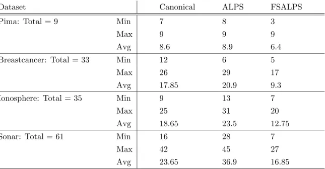
5.6 Minimum (Min), maximum(Max) and average (Avg) number of unique features in best solution tree for all runs . . . 55

5.7 Comparing mean difference between feature selection performed for each strategy at the 0.05 significance level using Tukey’s HSD ANOVA test for Breastcancer(⊗), Ionosphere(⊕), Pima( ) and Sonar() dataset for all 20 runs. An arrow points to the dominant strategy while a — means there is no significant difference between the two strategies. . . 55

5.8 Pearson Correlation Coefficients for Figure 5.3 . . . 57

5.9 Comparing mean difference between best solution tree-size for each strategy at the 0.05 significance level for Breastcancer(⊗), Ionosphere(⊕), Pima( ) and Sonar() dataset for all 20 runs. An arrow points to the dominant strategy while a — means there is no significant difference between the two strategies. . . 58

(9)

5.10 Comparing mean difference between initialization and evaluation time for each algorithm at the 0.05 significance level for Breastcancer(⊗), Ionosphere(⊕), Pima( ) and Sonar() dataset for all 20 runs. An arrow points to the dominant strategy while a — means there is no

significant difference between the two strategies. . . 64

6.1 Number of samples used per training class . . . 71

6.2 Canonical GP Parameters . . . 72

6.3 ALPS and FSALPS parameter settings . . . 72

6.4 Function set used for both representations. . . 73

6.5 Performance image legend. . . 76

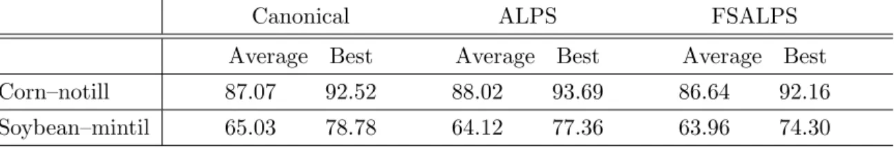
6.6 Classification accuracy for best evolved crop identifiers on the Indian Pines hyperspectral data . . . 78

6.7 Minimum (Min), maximum(Max) , average (Avg) and Standard Devi-ation (StD) number of unique objectives found in the solution set for each dataset. Total objectives considered for each dataset including ERC is: Corn–notill 201 and Soybean–mintil 201 . . . 79

6.8 Comparing mean difference between feature selection performed for each strategy at the 0.05 significance level for Corn–notill(⊗) and Soybean–mintil(⊕) . . . 79

6.9 Comparing mean difference between best solution tree-size for each strategy at the 0.05 significance level for Corn–notill(⊗) and Soybean–mintil(⊕) . . . 84

7.1 Comparing feature reduction (Features) and Maximum Classification Accuracy(Max CA) experimental results between FSALPS and CHCGA with Support Vector Machine(SVM) and Radial Basis Function(RBF) classifiers[9]. Pima (Total = 9), Ionosphere (Total = 35) . . . 88

7.2 Comparing performance of classifiers obtained in [71] with other re-ported results on Ionosphere(Total : 34), Pima Indians Diabetes (Pima, Total : 8), Sonar (Total : 60) and Wisconsin Breast Cancer –New (WBC New, Total : 30). For each of the datasets an ephemeral data set was added. . . 89

(10)

7.3 Comparing feature selection of some published strategies and FSALPS using Ionosphere(Iono., Total : 34), Pima Indians Diabetes (Pima, Total : 8), Sonar (Total : 60) and Wisconsin Breast Cancer - New (WBC New, Total : 30). For each of the datasets an ephemeral data set was added. . . 90 7.4 Comparing feature(spectral bands) selection of FSALPS corn–notil

(11)

List of Figures

2.1 A taxonomy of feature selection algorithms [35] . . . 13

2.2 GP Individual . . . 17

2.3 GP Crossover operation . . . 18

2.4 GP Mutation Operation . . . 19

4.3 Comparing parameter specified terminal probabilities with terminal selection during tree initialization. Accuracy is affected by population size, higher population produces more accurate results . . . 39

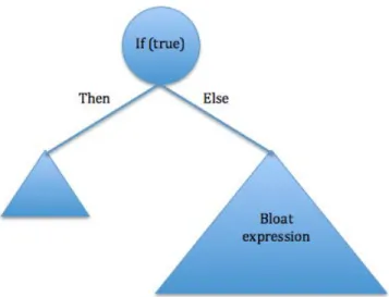
4.4 Bloat expression in a GP individual . . . 41

5.1 ALPS and FSALPS overtraining on Sonar dataset . . . 47

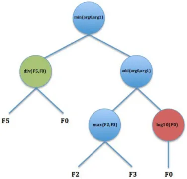
5.2 Evaluation of GP tree expression . . . 51

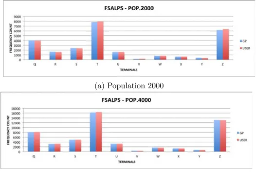
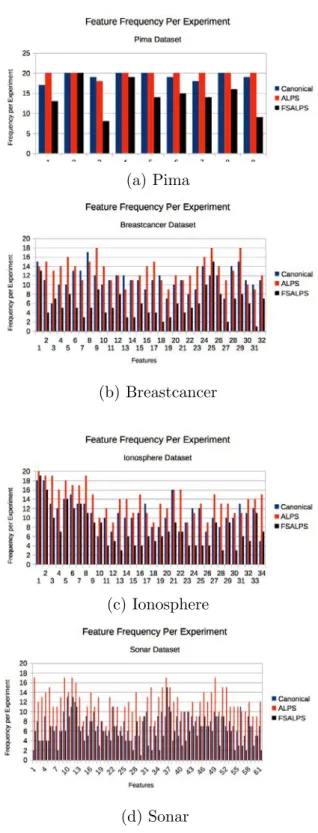
5.3 Histogram of cumulative feature used in solutions per dataset for 20 experiments . . . 56

5.4 Average individual size per generation for 250,000 evaluations . . . . 59

5.5 Initialization time using 250,000 evaluations . . . 62

5.6 Evaluation time using 250,000 evaluations . . . 63

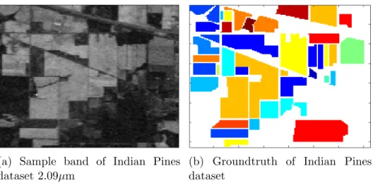
6.1 A sample spectral band from the Indian pins hyperspectral data and its ground truth image . . . 69

6.2 Hyperspectral bands . . . 74

6.3 Training performance plot . . . 75

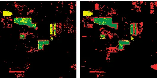
6.4 Classification results for map area using canonical GP with (a) 92.51% classification accuracy with 40.09% detection of total TP and 95.39% detection of TN (b) highest detection of TP with 71.65% TP and 88.94% TN . . . 76

(12)

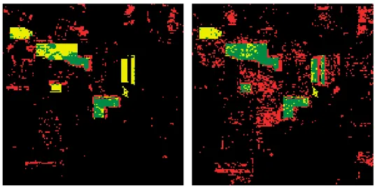
6.5 Classification results for map area using ALPS GP with (a) 93.69% classification accuracy with 37.06% detection of total TP and 96.78% detection of TN (b) highest detection of TP with 71.01% TP and 88.92% TN . . . 77 6.6 Classification results for map area using FSALPS GP with (a) 92.16%

classification accuracy with 58.81% detection of total TP and 93.98% detection of TN (b) highest detection of TP with 74.50% TP and 90.97% TN . . . 77 6.7 Percentage contribution of each feature per layer in the FSALPS–run

with minimum number of selected features. Layer 4 ended with 7 features testing classification accuracy of 80.48% . . . 80 6.8 Percentage contribution of features in Layer 0 of (a) FSALPS and (b)

ALPS. FSALPS is more stable than ALPS . . . 81 6.9 Tree growth using Corn–notill (a and b) and Soybean–mintil (c and d) 83 6.10 Initialization time using 250,000 evaluations . . . 85

A.1 ALPSGP on Pima Indians Diabetes dataset using two replacement strategies . . . 106 A.2 (a)Comparing ALPSGA Steady State and Generational replacement

strategy on a Max-Ones Problem and (b)Pima Indians Diabetes dataset using two replacement strategies . . . 107 A.3 ALPSGA Steady State and Generational Replacement strategies on

two Ageing Schemes . . . 108 A.4 Percentage contribution of each feature per layer in the FSALPS run

using Pima Indians Diabetes dataset. Evolution was initialized using equal probability settings for all features . . . 109 A.5 Percentage contribution of each feature per layer in the ALPS run

using Sonar dataset. Evolution was initialized with equal probability settings for all 60 features and performing periodic feature count and feature probability calculation . . . 110 A.6 Percentage contribution of each feature per layer in the FSALPS run

using feature frequency count of only L9 . . . 111 A.7 Percentage contribution of each feature per layer in the FSALPS run

on Pima Indians Diabetes dataset . . . 112 A.8 Training performance plot . . . 113

(13)

A.9 Pima: Percentage contribution of each feature in canonical GP run with (a) overall best individual had 9 features and 94.12% classification accuracy (b) minimum features had best individual with 7 features and 52.94% classification accuracy. . . 114 A.10 Pima: Percentage contribution of each feature per layer in the ALPS

run with (a–e) Layer 4 of best individual having 8 features and 88.23% classification accuracy (f) the best also individual scored the minimum number of features . . . 115 A.11 Pima: Percentage contribution of each feature per layer in the FSALPS

run with (a–e) Layer 4 of best individual having 9 features and 94.12% classification accuracy (f) Layer 4 of individual with minimum features had 3 features and 75% classification accuracy. . . 116 A.12 Breastcancer: Percentage contribution of each feature in canonical GP

run with (a) overall best individual had 13 features and 100.00% clas-sification accuracy (b) minimum features had best individual with 12 features and 96.43% classification accuracy. . . 117 A.13 Breastcancer: Percentage contribution of each feature per layer in the

ALPS run with (a–e) Layer 4 of best individual having 21 features and 100.00% classification accuracy (f) Layer 4 of individual with minimum features had 6 features and 89.66% classification accuracy. . . 118 A.14 Breastcancer: Percentage contribution of each feature per layer in the

FSALPS run with (a–e) Layer 4 of best individual having 6 features and 100.00% classification accuracy (f) Layer 4 of individual with minimum features had 5 features and 96.55% classification accuracy. . . 119 A.15 Ionosphere: Percentage contribution of each feature in canonical GP

run with (a) overall best individual had 14 features and 100.00% clas-sification accuracy (b) minimum features had best individual with 9 features and 77.78% classification accuracy. . . 120 A.16 Ionosphere: Percentage contribution of each feature per layer in the

ALPS run with (a–e) Layer 4 of best individual having 19 features and 100.00% classification accuracy (f) Layer 4 of individual with minimum features had 13 features and 88.24% classification accuracy. . . 121 A.17 Ionosphere: Percentage contribution of each feature per layer in the

FSALPS run with (a–e) Layer 4 of best individual having 11 features and 100.00% classification accuracy (f) Layer 4 of individual with min-imum features had 7 features and 88.89% classification accuracy. . . 122

(14)

A.18 Sonar: Percentage contribution of each feature in canonical GP run with (a) overall best individual had 27 features and 100.00% classi-fication accuracy (b) minimum features had best individual with 16 features and 70.00% classification accuracy. . . 123 A.19 Sonar: Percentage contribution of each feature per layer in the ALPS

run with (a–e) Layer 4 of best individual having 45 features and 100.00% classification accuracy (f) Layer 4 of individual with minimum features had 28 features and 70% classification accuracy. . . 124 A.20 Sonar: Percentage contribution of each feature per layer in the FSALPS

run with (a–e) Layer 4 of best individual having 27 features and 100.00% classification accuracy (f) Layer 4 of individual with minimum features had 7 features and 80.00% classification accuracy. . . 125 A.21 Average individual size per run for 250,000 evaluations . . . 127 A.22 Size of best individual per generation for 250,000 evaluations . . . . 128 A.23 Size of best individual per run for 250,000 evaluations . . . 129 A.24 Size of best individual per generation for 250,000 evaluations . . . . 130 A.25 ALPSGA Steady State and Generational Replacement strategies on

two Aging Schemes . . . 131

B.1 Performance plot for Soybean–mintil with (a) TP detection : 26.69% , TN detection : 90.45% overall performance : 78.78% (b) TP detection : 52.47% , TN detection : 82.94% overall performance : 77.36% (c) TP detection : 52.70% , TN detection : 79.14% overall performance : 74.30% . . . 140 B.2 Space analysis using logarithmic plot for generational growth in tree

size . . . 141 B.3 Corn–notil: Percentage contribution of each feature in canonical run

with (a) overall best individual had 39 features and 92.51% classi-fication accuracy (b) minimum features had best individual with 18 features and 91.96% classification accuracy. . . 143 B.4 Corn–notil: Percentage contribution of each feature per layer in the

ALPS–run with (a–e) Layer 4 of best individual having 48 features and 93.69% classification accuracy (f) Layer 4 of individual with minimum features had 31 features and 87.78% classification accuracy. . . 144

(15)

B.5 Corn–notil: Percentage contribution of each feature per layer in the FSALPS–run with (a–e) Layer 4 of best individual having 35 features and 92.16% classification accuracy. (f) Layer 4 of individual with min-imum features had 7 features and 80.48% classification accuracy. . . . 145 B.6 Corn–notil: Percentage contribution of each feature in canonical run

with (a) overall best individual had 21 features and 78.78% classi-fication accuracy (b) minimum features had best individual with 17 features and 64.91% classification accuracy. . . 146 B.7 Soybean–mintil: Percentage contribution of each feature per layer in

the ALPS–run with (a–e) Layer 4 of best individual having 56 fea-tures and 77.36% classification accuracy (f) Layer 4 of individual with minimum features had 29 features and 61.08% classification accuracy. 147 B.8 Soybean–mintil: Percentage contribution of each feature per layer in

the FSALPS–run with (a–e) Layer 4 of best individual having 20 fea-tures and 74.30% classification accuracy (f) Layer 4 of individual with minimum features had 7 features and 67.78% classification accuracy. 148 B.9 Number of times features were used in all 20 runs for Corn–notill in

(16)

Chapter 1 Introduction

Machine learning (ML) is a branch of artificial intelligence that deals with auto-matic induction of knowledge from data [54]. The 21st _{century has seen an}

exponen-tial growth[50] of high–dimensional data in bioinformatics, web/text data, biology, medicine, finance etc., necessitating the use of ML techniques such as GP and GA for data analysis. The pervasive nature of high dimensional data challenges present techniques used in data mining, pattern recognition and information filtering. Model construction in ML is used to induce hypotheses that can be learned from data. A hypothesis is a function that predicts classes from input features[50] and is referred to here as a classifier. High dimensional problems have large hypothesis space that usually results in an increased difficulty in selecting the most efficient hypothesis. Classification is one of the major tasks in data mining, and has to do with the use of features or attributes to predict class labels (outputs or targets)[63]. In [9], a feature is defined as “an independent measurable property of a process been observed”. In ML, features are used to generate models for classification. The number of features considered for a given problem has a direct bearing on the hypothesis space [54]. A linear growth in the number of features results in an exponential grow in the hypothe-sis space therefore a reduced feature vector reduces the hypothehypothe-sis space and increases the chance of discovering the most appropriate hypothesis. Feature selection (FS) is used to reduce the dimensionality of a given dataset. According to [61], relevant fea-ture subset selection for a learning systems improve understanding of the data, leads to the design of better classifier models, eliminate irrelevant data with benefits such as enhanced data visualization, reduced computational cost for constructing learning models and improve generalization of constructed models. Feature extraction (FE) on the other hand, deals with the discovery of composite features from an original feature vector that are more representative of the dataset. The newly discovered

(17)

CHAPTER 1. INTRODUCTION 2

tures (linear or non-linear combination of the original features) should score a higher prediction rate of the class labels. FS and FE are key preprocessing steps in machine learning.

Given that GP has a dynamic expressive ability, it can be guided using a fitness function to represent solutions for different problem domains. A GP classifier is an evolved GP expression that measures how a selected subset of features from the original feature vectors predicts the class label(s) for some data instances.

Evolutionary algorithms often converge on suboptimal solutions, as is the case for most stochastic algorithms. The problem of finding and optimal set of feature vectors out of an original set is NP complete [50, 9]. Feature reduction to a set of relevant features directly benefits machine–learning algorithms.

The age layered population structure (ALPS) strategy is used to overcome the problem of premature convergence in algorithms with elements of randomness in them. In ALPS, the regular introduction of new individuals into the population results in an evolutionary algorithm that is almost never converged but constantly exploring different parts of the fitness landscape [29] with an increased chance of landing on a global optimum solution. A number of published works have recorded the benefit of the ALPS system [29, 30, 59].

This research presents feature selection and ALPS (FSALPS) as a novel GP sys-tem that relies on the ALPS strategy to perform directed feature selection. FSALPS seeks to advance GPs ability to perform automatic feature selection by integrating knowledge of feature selection in the ALPS layers to control generation of new in-dividuals and genetic operations. In FSALPS, features with high discrimination of class labels are favored without forcing the EA system in premature convergence or limiting the ability of the EA system to explore relevant parts of the fitness landscape.

1.1 Goals and Motivation

The success of ML in database and knowledge discovery (DKD) tasks is largely de-pendent on the number of features or attributes considered for a problem[9]. An inefficient selection of input data will limit performance of machine learning tasks while a carefully selected data will significantly improve performance and enhance accuracy of prediction models. This explains why the number of variables consid-ered for a learning system affects the extent to which meaningful knowledge can be discovered. Most real world problems have huge volumes of data with noisy vari-ables (objectives). High dimensional data increases the hypothesis space, reduces the

(18)

classification accuracy of model construction algorithms and introduces the curse of dimensionality [50]. This can be overcome by applying preprocessing techniques in machine learning such as feature selection or feature extraction. The selective re-finement of feature variables involves elimination of noisy variables leaving a set of relevant variables that have significant impact on the measured process. Ann feature vector problem has an exponential solution space of 2n_{. A reduction of the original}

feature vector by k reduces the solution space to 2n/2k. A reduced feature set to relevant feature values leads to improved prediction accuracy and better tractability for large dimensional datasets. Reducing curse of dimensionality for DKD problems to computationally feasible problems open a new door to the discovery of meaningful knowledge from such datasets. This will advance ML in most research areas and could easily lead to potential breakthroughs in many application fields.

Population based heuristic search algorithms such as GA and GP have been used in classification problems in feature selection and construction. Due to its represen-tational superiority, GP is able to perform automatic feature selection while evolving a classifier. The evolutionary process favors GP tree expression that select a sub-set of feature variables (terminal symbols) that maximize the prediction accuracy of the classifier. The feature selection ability of GP is directly challenged by possible occurrence of bloat expressions in evolved individuals. Features in bloat expressions increase the overall score of frequency count of such features and might be misleading towards measuring feature relevance. Bloat expressions in canonical GP multiply as individual solutions increase in size due to genetic operations with a corresponding increase in space requirements as well as initialization and evaluation time.

We propose a novel evolutionary feature selection and classification strategy that uses the ALPS algorithm to evolve a classifier and perform feature subset selection with high classification accuracy. The approach is achieved by using ALPS to over-come the problem of premature convergence in canonical GP and simultaneously evolve feature subsets with high discrimination of class labels. Our proposed FSALPS strategy performs feature selection using ALPS GP towards dimensionality reduction. FSALPS uses a novel frequency–based feature–ranking system that will be used to control domain specific genetic operations and to determine probability of feature assignment to new randomly created individuals. The proposed meta–heuristic will be tested on high dimensional benchmark datasets and compared to canonical GP, ALPS GP and other statistical strategies used in classification, feature selection and construction. Combining ALPS search power with GPs dynamic tree encoding to perform feature subset selection will lead to a significant improvement in aspects

(19)

of classification problems involving high dimensional datasets. We will show that FSALPS GP significantly reduces the number of features whiles maintaining or im-proving classification accuracy. We will simultaneously exploit GPs default encoding for the construction of a classifier system to measure performance of the selected fea-ture subset. This will effectively reduce the computational effort needed to design a classifier system as compared to other feature selection strategies that rely on external classifiers.

1.2 Thesis Structure

Chapter 2 reviews relevant background information on topics such as classification, feature selection, heuristic and population based algorithms, genetic programming and the ALPS strategy. We will continue with a literature review of related research in feature selection in Chapter 3. Chapter 4 builds on the ALPS algorithm by intro-ducing a feature selection paradigm named FSALPS. In Chapter 5, we will discuss and compare the performance of canonical GP, ALPS GP and FSALPS strategy on feature selection and classifier construction using multiple ML datasets. We will also examine a high dimensional hyperspectral data to provide further evidence of the fea-ture selection ability of FSALPS in Chapter 6. In Chapter 7, FSALPS is compared to related works. Concluding remarks and future research is presented in Chapter 8.

(20)

Chapter 2 Background

2.1 Introduction

In the fields of pattern recognition, data mining and knowledge discovery, feature re-duction influences the quality of learning models constructed from high dimensional data. Feature selection eliminates features that offer little or no contribution to the class label. For instance, a demographic data that is to be used to predict the occur-rence of a particular disease within a population may contain features or attributes that are irrelevant to the disease condition. The removal of such irrelevant or noisy attributes will enhance performance of learning models and significantly reduce the hypothesis space needed for model construction. Feature selection has been used as a pre–processing technique for function approximation, classification and cluster-ing, using learning systems designed in neural networks[8], regression models[10] and decision trees[16]. A number of classification algorithms have been used in feature selection and feature construction.

In this thesis, we will compare existing and new evolutionary techniques for feature selection and classification on supervised learning tasks. A number of methods have been developed for feature selection or variable elimination and are broadly classified into filter, wrapper and embedded methods[50]. Feature reduction as studied in machine learning can be broadly classified into two main problem domains –supervised and unsupervised learning.

(21)

CHAPTER 2. BACKGROUND 6

2.2 Classification

Classification is a major task in supervised machine learning [54] and has been applied to a wide range of problems such as credit scoring, bankruptcy prediction, medical diagnosis, pattern recognition, text categorization, and software quality assessment. [20]. The goal of classification is to accurately predict discrete class labels using predictor values or feature variables. Prediction rules are applied to pre–classified training examples such that the rule with the highest prediction accuracy with the ability to generalize other unseen test examples is preferred. Classification data could be as simple as in binary classification, where the target values to be predicted are two e.g. high credit rating or low credit rating, or diabetic or non–diabetic. It could also be as complex as multi class classification involving identification of numerous class labels as seen in multiple target identification problems. In [57] an example of multi classification is given as case where a loan applicant could fall within any of the following credit ratings: low, medium, or high credit risks. The credit rating for each client will be treated as the target while the other attributes (e.g. home ownership or rental and/or location of apartment/building, number of years of rent, type of employment, investments, borrowing records etc.) will be treated as the predictors [or features]. Given the above problem, a classification algorithm uses a pre–classified training example to generate a highly generalizable rule to relate most/all features to the respective credit rating. Learning algorithms such as decision tree learning algorithm, Support Vector Machines, Neural Network, k–NN, Naive Bayes, General-ized Linear Models and Support Vector Machine (using linear and Gaussian kernel functions), GP and GA have been used as classifiers in various classification tasks [20, 54, 57].

2.2.1 Unsupervised Learning

In unsupervised learning, the data instances have no distinction of types based on input and output variables [50]. Since there is no known output, unsupervised learning excludes training. The goal, therefore, is to discover intrinsic relations or group data instances based on naturally existing affinities between attributes [50]. Clustering and association discovery are examples of unsupervised learning.

(22)

2.2.2 Supervised Learning

In supervised learning, features (attributes) are distinctively categorized into depen-dent (output) and independepen-dent (input) variables [50]. The dependepen-dent variables (class variables) are to be predicted from the independent variables by training the predic-tion algorithm (or classifier) on the data instances. Regression and classificapredic-tion are the two main categorizations of supervised learning. In regression there are contin-uous–valued output to be predicted whilst in classification, the output values to be predicted are discrete.

2.3 Feature Selection and Feature Extraction

In [9], a feature is defined as “an independent measurable property of a process been observed”Noisy attributes in data increase the complexity of the learning space and reduce performance of learning algorithms with corresponding high computational requirement in data analysis and machine learning. Feature selection is the process of refining input data by removing irrelevant and/or redundant features[50]. Feature selection deals with selection of a subset of relevant features (variables) from an input data. Feature selection does not produce new features – all selected features are subsets of the original feature vector.

For a data set D containing m features, a feature selection algorithm selects a subset of n features by eliminating irrelevant and redundant features such that it improves or retains the prediction accuracy of the classifier algorithm. In [15], feature selection problem is defined as: given the original feature vector ofY (Equation 2.1) and a training set L, invent a representation X (see Equation 2.2) derived from Y that maximizes some criterion J(X) (see equation 2.3) and is at least as good as Y with respect to that criterion.

Y ={yi|i= 1, ..., D} (2.1)

X ={xi|i= 1, ..., d;xi ∈Y}d≤D (2.2)

J(Xopt) =maxX⊆Y,|X|=dJ(X) (2.3)

The criterion J(X) is a model or classifier which is used to measure the predictive accuracy of the selected feature subsetX. Feature selection algorithms are compared based on performance criteria such as simplicity, stability, number of reduced features, classification accuracy, information gain, storage and computational requirements. In

(23)

[9, 20] a number of feature–selection algorithms have been compared on some high dimensional benchmark datasets covering various application areas such as biology, medicine, finance, law, bioinformatics and engineering.

Feature extraction involves the discovery of interesting hidden relationships be-tween original feature vectors. The newly constructed features are linear or non–linear combinations of existing features. The newly formed composite features are fewer, clearer, easy to visualize, more representative of the problem and much more efficient for model extraction. As an example, when estimating the cost of life insurance, an insurance company will like to factor vulnerability of a person to some major disease factors. Attributes such as the height or weight of an applicant could be readily avail-able to the insurance firm. However those attributes in themselves do not necessarily measure any major health risk. On the other hand, an implicit derivation such as the weight to height ratio is crucial to some health risk factors such as obesity –making the new composite feature more valuable than the original features. Even though this attribute will not be explicitly available, the formulation of such key relations between existing attributes is more meaningful to the insurance company for potential health risks.

EAs can be used for the automatic construction of linear/non–linear combinations of features to form a smaller subset of features with improved predictability. GP construct new features by using its tree structure encoding of terminal and function sets to form a linear or non–linear relationship between the original or other composite features. When using GP for feature extraction, the value at the root node of an evaluated GP expression is considered as a new feature. This feature is an implicit derivation from the original feature vectors. Thus, an evaluated GP tree reveals a complex or simple relationship between existing feature vectors making the GP tree a composite feature. The newly created composite features can be used separately or combined with the primitive attributes (original feature vectors) to form a new feature vector.This unique property of GP makes it a suitable algorithm for data mining problems.

2.3.1 Filter Method

In the filter method (see Algorithm 1), feature search method and feature subset selection criterion are independent of the learning algorithm used in the final con-struction of the classifier [50]. This preprocessing technique ranks features before applying the classifier [or predictor] to the highly ranked features. Ranking methods

(24)

are applied to an original feature vector to score feature values based on relevance, which is then used to filter out redundant, irrelevant, and noisy attributes. A criterion is used to determine the rank of a feature using a suitable ranking criterion to select those that meet a predetermined threshold. As an example, a credit firm will want to know key characteristics (or attributes) of clients that determine their credit wor-thiness. Attribute importance is used to rank each independent feature to produce a value that measures how strong (predictive significance) an attribute contributes towards discriminating the credit worthiness (class label) of a client. In determining feature relevance a unique feature must contain relevant information about the dif-ferent classes in the data [9]. According to [9, 44], features that have no influence on the prediction of the class labels are irrelevant and can be discarded. One way of obtaining feature ranking is by measuring inter–feature correlation. Degree of cor-related features provide some information on inter–feature dependencies. According to [9], “when two or more features are strongly correlated, one is enough to describe the group and the dependent feature provides no extra information for discriminating the class labels”. A good feature can be independent of the remaining features but must provide high discrimination for the various class labels. Noisy and redundant features can degrade accuracy of the learning models leading to poor generalization or over-fitting. Over–fitting is a case where the learning model performs well on the training data but poorly on test data. In [9, 52] information gain, minimum de-scription length, maximum relevance, feature-correlation and mutual information are listed as other ways to rank features.

(25)

Algorithm 1 Filter Method (from [51])

1: procedure FILTER()

2: Y(F0, F1, ..., Fn−1) B data set D containing n features

3: S0 B initial subset

4: X _B invent a representation X that maximizes some criterion J(X) 5: Sbest ←S0 B initialize Sbest

6: µbest ← apply heuristic(S0, Y, J) B apply J toS0

7: while (!TerminationCriteria()) do

8: S← create subset(Y) B apply a heuristic to create subset 9: µ← apply heuristic(S,X,J)_B gets classification accuracy ofS

10: if µ.betterT han(µbest)then

11: µbest ←µ

12: Sbest←S

13: end if

14: end while

15: µ ←classification accuracy(S,X,J) _Bgets classification accuracy of S

16: return Sbest

17: end procedure

2.3.2 Wrapper Method

The wrapper method (see Algorithm 2) uses the same learning algorithm used in constructing the final classifier to evaluate feature subsets. The classifier is “wrapped around”a feature–subset search algorithm to determine the subset with the highest predictability to maximize the performance of the classifier.

In a large dimensional data, as N grows exhaustive evaluation of all possible feature subsets become NP–hard. With an exponential growth in feature subsets, exhaustive direct search algorithms such as branch and bound require high computa-tional time and are often intractable as compared to suboptimal search algorithms. Examples of non-exhaustive algorithms applied in the generation of feature subset are the sequential selection algorithms and heuristic search algorithms such as GA. The feature generation process is followed by an external learning algorithm that measures the performance of a selected subset.

(26)

Algorithm 2 Wrapper Method (from [51])

1: procedure WRAPPER()

2: Y(F0, F1, ..., Fn−1) B data set D containing n features

3: S0 B initial subset

4: X _B invent a representation X that maximizes some criterion J(X) 5: Sbest ←S0 B initialize Sbest

6: µbest ← classification accuracy(S0, Y, J) Bapply mining algorithm J to S0

7: while (!AccuracyImproved()) do

8: S← create subset(Y) B apply a heuristic to create subset

9: µ← classification accuracy(S,X,J) _B gets classification accuracy ofS

10: if µ.betterT han(µbest)then

11: µbest ←µ 12: Sbest←S 13: end if 14: end while 15: return Sbest 16: end procedure

Sequential selection algorithms start with an empty or full feature set and iter-atively add or remove features until a feature subset with maximum classification accuracy is obtained. In the sequential forward selection (SFS) [9] algorithm, the subset generation begins with an empty list, and iteratively adds one feature at a time while choosing the next best feature that yields higher prediction accuracy of the class labels. Sequential backward selection (SBS) starts with a full list of the feature vector and iteratively removes features while accepting the elimination that yields the list change in prediction accuracy of the remaining feature subset. The interested reader is directed to [9] for other variants of SFS and SBS, such as sequen-tial floating forward selection, adaptive sequensequen-tial forward floating selection, adaptive sequential backward floating selection, and plus-L-minus-R.

In some related works, GA was used for feature generation and decision tree[?], k-nearest neighbor (KNN)[37] classifier. [53, 39] used simulated annealing algorithm and a regression based evaluation function for feature subset selection. Alba et all [2] used a hybrid particle swarm optimization (PSO) and GA feature generation and a support vector machine (SVM) classifier. The wrapper method is reported to have better results than the filter approach even though its prone to over-fitting and high computational requirements [9].

(27)

2.4 Embedded Method

The embedded method[6] integrates the feature generation strategy and the classi-fication of the quality of the selected subset into the learning algorithm, thus the link established between feature selection and classification is stronger than in the wrapper method [22]. This leads to a combination of the advantages of filter and wrapper based methods with a reduced computational time [9, 22]. The implicit feature generation built into learning algorithms such as decision tree induction algo-rithms makes CART, ID3 and C4.5 embedded learning methods[41]. By extension, the GP representation based on decision tree induction algorithm also qualifies as an embedded method.

2.5 Evolutionary Algorithms

Heuristic search algorithms include sub–optimal algorithms such as genetic algo-rithms, genetic programming, particle swarm optimization, ant algoalgo-rithms, and simu-lated annealing. The taxonomy of feature selection algorithms is shown in Figure 2.1. Evolutionary Algorithms such as GA and GP borrow principles of natural selection and survival of the fittest from Darwinian theory of evolution to breed a population of feasible individuals using genetic operations such as crossover and mutation. EAs perform parallel evaluation of possible solution sets in the search space by using an objective function that drives the entire search process towards the global optimum. From Algorithm 3, suboptimal population based EAs have the following general char-acteristics:

(a) The use of a population of individuals (see line 2 of Algorithm 3), which repre-sent a complete or partial solution of the optimization problem. Each solution is defined to meet some predetermined constraints.

(b) A keep–alive evolution process ((see line 4−8 of Algorithm 3)) that breeds new offsprings to replace existing parents until termination criteria is reached. New offsprings are created using genetic operators like crossover and mutation. Crossover swaps a sub–part of the genetic materials from two parents to create two offsprings and mutation randomly alters a sub–part of a parent to create one offspring.

(c) EAs breed a population of solutions and perform parallel evaluation of the solu-tion sets in its search space by using an objective funcsolu-tion that drives the entire

(28)

search process towards a global optimum. Fitness based individual measure-ment criteria that assign a value to an individual based on how best it answers the problem. Fitness is used as a criterion for probabilistic selection of parent chromosomes that take part in breeding. The fitness-based selection ensures that most highly fit (strong) individuals pass their genetic material to the next generation.

By using genetic evolutionary operators, and a measure of fitness, EAs are able to perform exploitation and exploration through the search space and drive the entire search process towards promising regions of the fitness landscape. EAs are effective meta–heuristics for searching through large search spaces [14, 16]. A stopping criterion is made on the assumption that individuals are always valid and satisfy all problem constraints. Individuals are bred and evaluated until the EA system satisfies any of these stopping criteria:

(a) The ideal individual has been discovered. This is the individual that correctly classifies all training instances.

(b) The EA system is stuck in local optima such that continuous evolution does not move the entire population from mediocre local optima.

(c) The number of generations specified for a run has been completely exhausted.

Figure 2.1: A taxonomy of feature selection algorithms [35]

A replacement strategy is used to determine how a new population is produced to replace an old population. The two most popular replacement strategies used in

(29)

breeding new population from the existing population are generational and steady state replacements. In generational replacement, individuals in a population are subjected to genetic operations to produce offspring for each subsequent generation. The newly bread population replace the parent population. This new population may include elite individuals that were copied from the old population. The new population of individuals is used to produce the next generation until a termination criteria is met. In a steady state replacement, an offspring individual competes with parents using survival of the fittest or evolutionary survival strategy. The most often used individual replacement strategy is the reverse tournament where an offspring replaces the worst tournament individual.

(30)

Algorithm 3 Simple GA

1: procedure GEN GA()

2: Population ←CreateInitialPopulation _B randomly 3: Generation ← 0

4: while !( FoundIdealIndividual(j) | TimeIsUp() | MAX(Generation) ) do

5: EvaluateFitness(Population)_B Each individual in Population 6: Population← BreedNewPopulation()

7: Generation++

8: end while

9: end procedure

1: procedure BreedNewPopulation()

2: NewPopulation _B initialize new population 3: i ← 0

4: SelectionOperation ← {Mutation, Crossover, Reproduction} 5: for i < popSize do _BpopSize is user specified

6: GeneticOperation ←ProbabilisticalSelect(SelectionOperation) 7: if GeneticOperation = Reproduction then

8: j ← SelectOneIndividualBasedOnFitness(Population) 9: k = Reproduction(j)

10: end if

11: if GeneticOperation = Crossover then

12: j ← SelectTwoIndividualBasedOnFitness(Population) 13: k = Crossover(j)

14: end if

15: if GeneticOperation = Mutation then

16: j ← SelectOneIndividualBasedOnFitness(Population) 17: k = Mutation(j) 18: end if 19: i += k.size() 20: NewPopulation ←k 21: end for 22: return NewPopulation 23: end procedure

(31)

2.5.1 Genetic Programming

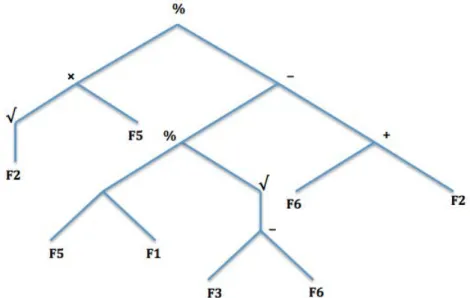
GP [38] is a special case of GA that uses a tree data structure to represent an indi-vidual. GP is very flexible and can be adapted to represent various complex patterns from a wide range of domain knowledge. GP was initially introduced with the in-tention of evolving computer programs. The subject area has expanded to include evolution of mathematical expressions and rule based systems[20]. This expressive power makes it possible to develop dual representations for feature selection and clas-sifier design. In this work, GP is exploited for feature selection and classification by evolving individuals with non–terminal symbols using functions and operations and terminal symbols using the original feature vector. A GP individual is a complete or partial solution represented using a parse tree where constants and variables denote terminal symbols and operators and functions denote non–terminal symbols. Leave nodes correspond to terminal symbols and internal nodes correspond to non–terminal symbols. By the above definition, a function set is the set of all allowed non-terminal symbols and terminal set is the set of all allowed terminal symbols. GPs flexibility can be extended to the construction of various classifiers with representational for-malisms such as decision trees, classification rules, discriminant functions, artificial neural networks and many more [20]. The automatic feature selection performed during GPs evolution results in an individual with higher prediction accuracy and contributes to better interpretability of resulting solutions. GP also has the ability to perform automatic feature extraction using a linear or non linear combination of features as sub–trees in a GP individual. A GP language must satisfy the following two conditions:

(a) Sufficiency: this means the GP language including terminal and function sets are enough to evolve a solution for the target problem.

(b) Closure: this is loosely defined as a case where each non-terminal function is able to operate error–free on all values parsed as an input. However in a strongly typed GP language, non–terminals only operate on values that are of the same type as the type of the child node(s). For strongly typed problems, more computational time is used during tree initialization and genetic opera-tions to guarantee type check consistency of nodes in the parse tree.

The specific representation adopted in this thesis is the binary tree based in-dividual representation. A set of inin-dividuals make up a population (P) such that

(32)

which is translated into the lisp s–expression

(% (x(√x2)x5)( (−(% (+x5x1)(√(−x3x6))) (+x6x2)))

For feature selection problems, terminals are the problem features and are usually combined with randomly generated constants such as an ephemeral constant (ERC). Function sets are operands (such as ∗, +, −,√ in Figure 2.2), which perform opera-tions on the terminals and results of other non–terminals. Tree sizes usually increase in depth as evolution progresses. When two individuals are of the same fitness, the smaller is preferred so as to evolve simple and portable solutions.

Figure 2.2: GP Individual

The representational power of GP allows implicit feature selection from the ter-minals of the GP tree while the entire tree can be evaluated to represent an extracted feature. In Figure 4.2, the feature subset is the collection of unique terminal symbols in the set{x1, x2, x3, x5, x6}. On the other hand, the root value of the GP expression could be evaluated as a new feature, which becomes an implicit derivation from the original feature vectors.

Crossover Operation

During crossover (see line 11−14 of Algorithm 3), two parent individuals are selected from the population using fitness-proportional selection. A random crossover point is selected from both parents and the sub trees rooted at those nodes are swapped between parents. A typical crossover operation breeds two new offspring as seen in Figure 2.3c and Figure 2.3d from two parent individuals Figure 2.3a and Figure 2.3b. Crossover operations result in exploration of new parts of the fitness landscape.

(33)

This is due to the likely combination of genomes from different parts of the fitness landscape.

(a) Parent 1 (b) Parent 2

(c) Child 1 (d) Child 2

Figure 2.3: GP Crossover operation

Mutation Operation

In GP, mutation is the process of randomly generating a tree and rooting it on a random node in a parent GP tree (see line 15−18 of Algorithm 3). The parent tree is selected through tournament selection using fitness/random–based selection. In Figure 2.4a, a random node is selected and the randomly constructed tree (see Figure 2.4b) is rooted on the parent individual to form an offspring individual as seen in Figure 2.4c. Mutation is exploitative as it seeks to refine fitness within a particular region of the fitness landscape by rearranging the genes.

(34)

(a) Parent with randomly selected mutation point

(b) Randomly generated sub-tree

(c) Parent rooted with randomly generated sub-tree (Figure 2.4b)

Figure 2.4: GP Mutation Operation

2.5.2 Age Layered Population Structure

The Age Layered Population Structure (ALPS) introduced by Hornby[29] is a novel meta-heuristic that seeks to reduce the problem of premature convergence in stochas-tic algorithms. In ALPS, age is used as a property of individuals to restrict competi-tion and breeding in the populacompeti-tion. ALPS segregates the populacompeti-tion of individuals into age-layers. Age is measured by how long an individual’s genotypic material has been evolving in the population. Hornby[29, 30] applied the ALPS strategy in various problem instances and recorded results that outperformed canonical EA.

An aging scheme (see line 2 in Algorithm 4) is used to separate individuals into age layers (see Table 2.1). These values are multiplied by an age gap parameter to determine the maximum age per layer. Given an exponential aging scheme with an age gap of 10 and 6 layers, the maximum ages for the layers will be 10,20,40,80,160,320. Individuals within a layer are not allowed to outgrow the maximum allowed age

(35)

Algorithm 4 Pseudocode for ALPS

1: procedure ALPS GEN()

2: AgeScheme ← SelectAgeingScheme() 3: layers ←CreateLayers(AgeScheme) 4: i ← SequentialLayerSelection(layers). 5: init:

6: if BottomLayer(i) & reinitializationModethen 7: j ← CreateNewRandomGenome().

8: else

9: if BottomLayer(i) & TooOld(i) then 10: reinitializationMode ← true 11: j ← CreateNewRandomGenome(). 12: else 13: reinitializationMode ← false 14: j ← CreateNewRandomGenome(). 15: end if 16: end if 17: stop:

18: if !( FoundIdealIndividual(j) | TimeIsUp()) then

19: returnfalse 20: end if 21: loop: 22: goto init. 23: childId ←SelectSlotNextGeneration(i) 24: j ← CreateChild(childId). 25: EvaluateChild(j) 26: TryMoveUp(i,j ) 27: goto stop. 28: end procedure 1: procedure TryMoveUp(i, j) 2: if TopLayer(i)then 3: k ←FindVictim(i,j). 4: TryMoveUp(i,k) 5: else 6: k ←FindVictim(i+1,j) 7: TryMoveUp(i+1,k) 8: if Empty(k)then 9: i← j 10: else 11: Discard(k). 12: end procedure

(36)

for that layer. Rather, an attempt is made to move such individuals to the next higher layer (see line 26 in Algorithm 4). Unsuccessful migrants are destroyed. The maximum age per layer allows evolution to proceed long enough in the preceding layer before individuals are old enough to migrate to the next available layer. It also allows individuals to improve in fitness before being pushed to the next higher layer. The last layer on the other hand, has no age limit, hence allows for the accumulation of the best individuals. According to [29], an individual in the last layer is only guaranteed to remain there provided it is the global optimum or else it will be replaced by other highly fit individuals from the lower layers. An ALPS system is characterized by the following:

(a) At initialization, individuals are assigned an age of zero (see lines 6− 8 in Algorithm 4).

(b) At regular intervals (determined by the age–gap) new individuals are initialized in the bottom layer (see lines 6−8 in Algorithm 4). This is when current individuals in layer 0 might have aged into layer 1.

(c) The age of an Individual selected for genetic operation is incremented once per generation for which the individual was used as a parent.

(d) Offspring of parent individuals are assigned the age of the oldest parent plus one.

(e) Breeding is only allowed between adjacent layers using a selection pressure. When breeding, a parent is selected with a probability of n% from the current layer and (100−n)% from the lower adjacent layer (e.g. in layer 1, parents are selected from layer 1 and 0, in layer 2, parents are selected from layer 2 and layer 1. This novel process is used to control breeding and competition between individuals in the layers and facilitate the transfer of genotypic materials from lower layer individuals to the higher layers.

(f) Replacement (see line 26 in Algorithm 4) occurs within the population of the active layer. The breeding process enables individuals to age smoothly through higher layers.

(37)

Table 2.1: Examples of Age scheme for ALPS [29]

Aging-scheme 0 1 2 3 4 5 6 8

Linear 1 2 3 4 5 6 7 8

Fibonacci(n) 1 2 3 5 8 13 21 34 Polynomial(n2) 1 2 4 9 16 25 49 64 Exponential(2n) 1 2 4 8 16 32 64 128

Each successive layer is opened when evolution has occurred for as long as the maximum allowed age for the preceding layer. Thus with the above aging scheme, layer 1 will be opened for evolution at the end of generation 10, layer 2 is opened at the end of generation 20, and so on. The layered approach of evolution does not only restrict competition between individuals in the entire population but also serves as a way of transferring genotypic materials from different fitness basins to higher layers. In ALPS, the bottom layer is regularly replaced with randomly generated individuals. The periodic introduction of such individuals in the bottom layer results in an EA that is never completely converged [29]. By using age to restrict breeding, it reduces the possibility of highly fit old individuals dominating the evolution process, which most often leads to early convergence in canonical EA. Random number seeds are varied for each initialization of base population, which often results in the new population starting off from a new fitness basin. Through the explorative and exploitative nature of genetic operations, breeding could produce an offspring individual that takes the entire population from mediocre local optimum. Each bottom layer restart in ALPS creates a population clustered around a different fitness basin [29], thus the resultant ALPS population increases exploration of the fitness landscape.

When an individual reaches its maximum allowed age in a layer, it will move to the next higher layer. Since a constant population is maintained in all layers, an individual in the next higher layer will have to be displaced to make room for a new individual. In the generational replacement strategy, individual aging in a layer and inter–layer individual movements are synchronized on the condition that when applying selection pressure to pick parents from two layers, a parent selected from a lower layer is not aged. However in steady state replacement, various replacement strategies are adopted for inter–layer replacement. The new individual arriving from the next lower layer is only allowed to displace the weakest tournament individual in the higher layer otherwise it is destroyed. Different replacement strategies such

(38)

as replacing population weakest, reverse tournament, random, nearest fitness, etc., could be adapted to the ALPS system inter–layer individual migration.

(39)

Chapter 3 Related Work

3.1 Dimensionality Reduction

Meta-heuristics and approximate search algorithms provide suboptimal solutions to NP complete problems using minimal computational resources when compared to direct search algorithms[7]. Suboptimal algorithms have been used for dimensionality reduction on varied benchmark datasets with good classification accuracy and reduced computational requirements[9, 20]. In [20], a methodology is proposed that uses GP to perform feature selection and test the resultant features on a GP constructed classifier. The approach involves construction of a classifier that has n trees for an n–class problem. Dash and Liu [14] use a fitness measure to increase classification accuracy of k–NN classifier while reducing the number of selected features. The accuracy of the k–NN classifier is compared to other statistical methods of feature extraction such as linear discriminant analysis (LDA) and principal component analysis (PCA) [70].

Smith et al. [71] use GP and GA for feature extraction and feature selection respectively as a preprocessor for a C4.5 decision tree–learning algorithm. An indi-vidual is represented using automatically defined functions (ADFs) such that each individual is made up of separate trees [71]. An ADF is constructed from multiple features and a tree in an ADF is evaluated to produce a newly constructed feature. A GA system is used to evolve a feature subset from the new feature vectors by selecting from the extracted and original features. The resultant feature subset from the hy-brid EA system is tested using a C4.5 classification algorithm. The approach proved more successful than direct application of the standard C4.5 decision tree–learning algorithm on the same dataset. Similar benefits were recorded when the dual pre-processing strategies were performed before using k–NN and Na¨ıve Bayes classifiers. [58], [40] and [18] used C4.5 decision tree learning algorithm as a classifier for a GP

(40)

CHAPTER 3. RELATED WORK 25

feature construction problem.

Oechsle et al. [56] separate feature selection and feature extraction stages and used GP to evolve them independently on a vision problem. The GP classification methodology involved evolution of a set of partial solutions for a single class. This enables the use of GP for classification of high multi–class data and is reported to be faster than conventional GP. In [40] ECJ GP is used for feature construction and feature selection using C4.5 decision tree classifier implemented in WEKA [25]. Lin et al.[49] used a multi–population layered GP to perform feature selection. Two methods of feature selection are proposed in their work. The first method seeks to penalize individuals with high number of features by reducing the fitness values of such individuals. The second method assigns weight (based on feature relevance) to features during evolution; the assigned weights determine survivability of features during evolution. In the implementation of their layered GP [49], best individuals from each sub–population in a layer are considered as an extracted feature. Thus the number of extracted features is limited to the number of sub–populations considered in a layer. These sub–populations have no communication between them. New features extracted from lower layers are combined with existing features to form training set for the next higher layer.

The performance of some feature selection and classification algorithms were com-pared in [9, 20]. This far, no clear algorithm has emerged dominant for all feature selection problems and results often differ based on considered dataset. Piotr et al. [23] compared feature selection algorithms used in the analysis of chemical data. The results found random forest and support vector machine with recursive feature elimi-nation as superior to other considered strategies. The reader is referred to [9], where a number of feature selection and classification algorithms are compared based on prediction accuracy and reduced feature set.

Badran et al.[3] used a multi-objective GP to perform feature extraction as a preprocessing stage to a multi-class problem. This involved the reduction of the orig-inal dimensionality space to a new reduced and optimized multi-dimensional decision space. Thus, Bedran et al. [3] and Lemczyk et al.[45] used GP to handle a multi-class dataset by addressing the classification problem through task decomposition.

The layered GP considered in ALPS restricts communication between some lay-ers. In [49] terminals always have positive weights and the original features are always considered with the extracted features when performing generational weight assign-ment. We do not penalize individuals with many features as done in [49] but rather, in the FSALPS GP system, we allow natural evolution of feature ranks, such that

(41)

irrelevant features gradually disappear under evolutionary pressure.

3.2 Classification

In supervised learning, classification [54] involves the use of an inductive learning method to predict class labels based on information about other features. The goal is to develop a rule (classifier) that assigns each feature vector to a discrete class label. In [9], a classifier is a model encoding a set of criteria that allows a data instance (feature vector) to be assigned to a particular output (class label) depending on some selected features from the data instance. The pre–classified data is divided into train-ing and test set. The classifier is trained on the traintrain-ing example to maximize the number of output scores predicted (correctly categorized) using the input feature vector. The classifier with the highest score of class labels is tested on unseen data (testing example) for its generalizability. A good performance on test example also shows that there was no over–training. Commonly used classifiers are the decision tree–learning algorithm, C4.5[54], k–nearest neighbor algorithm [54], Naive Bayes [46] and other statistical methods such as linear discriminant analysis (LDA)[27] and Prin-cipal component analysis (PCA)[70]. Support vector machines (SVM) represents the various samples as points in space. According to [23] these points are optimally sepa-rated by hyper–planes such that unique classes have their samples widely sepasepa-rated as much as possible.Given two or more group of samples, LDA [27] finds linear relations between features by maximizing inter–group variance whilst minimizing intra–group variance. Although LDA is simple to implement and often produce good results when the input features are linearly separable, it often does not produce good results on multi–classification problems [23]. PCA is a widely used feature extraction technique derived from linear algebra. It uses a non–parametric method for dimensionality re-duction by extracting interesting relationships between existing feature vectors. The interested reader is referred to [70] for a detailed discussion on PCA. In [9, 20], some criterion used for classifier evaluation include:

(a) Classification Accuracy. It is a measure of the number of correctly classified training examples against incorrectly classified training examples.

(b) Generality: ability of selected classifier to score high on unseen data.

(42)

GP can evolve classifiers for binary and multi-class problems. Lemczyk et al.[45] decomposed a multi-class problem using GP and a coevolutionary strategy to evolve classifiers through task decomposition. Their strategy proved very effective on three high-dimensional multi-class datasets.

3.3 Hyperspectral Classification Using GP

GP has the capacity to handle large dimensional datasets. For instance in [43], Lang-don used GP to address a large attribute space by reducing the number of features required to describe a cancer diagnosis dataset from a million to 5. Evolutionary computation has many uses in classification, dimensionality reduction and spectral band sub-set selection on hyperspectral datasets. We will investigate the performance (dimensional reduction and classifier construction) of canonical GP, ALPS and Fea-ture Selection ALPS (FSALPS) on a high dimensional hyperspectral dataset. Yin et al.[79] used a modified evolutionary technique —immune clonal strategy to per-form band selection of hyperspectral image obtained from Washington DC Mall and Northwest Tippecanoe County. Bazi et al.[4] and Zhou et al.[80] applied a genetic optimization framework for automatic feature selection and parameter optimization for an SVM classifier on hyperspectral remote sensing images. In a related work, Li et al.[47] used the hybrid strategy GA–SVM with a branch and bound algorithm (in the post–processing phase) on a hyperspectral image. [81] used the wrapper based fea-ture selection strategy with GA and SVM classifier to reduce the number of spectral bands of a HYPERION hyper spectral image from 198 to 13. The GA system simul-taneously optimized the SVM kernel parameters, resulting in an improvement in the classification accuracy of the reduced spectral bands. Other proposed dimensionality reduction algorithms used for feature reduction and classification of hyperspectral im-age are the GA based local–fisher’s discriminant analysis proposed by Cui et al.[12], GA based feature mining techniques for feature selection and feature extraction[36], and the use of artificial neural networks on remote sensing data[1].

Alex dos Stantos et al.[17] used a content–based image retrieval technique that uses GP to obtain composite descriptors from remote sensing images with an op-timum–path forest classifier. Their technique was successfully used in the identi-fication of crop regions on remote sensing images. Due to GPs adaptive learning technique, canonical GP performed a dual function of automatic evolution of classi-fiers and feature reduction using spectral imagery[62]. Ross et al.[65] applied GP to the Cuprite hyperspectral image for the automatic evolution of mineral identifiers.

Feature Selection and Classification Using Age Layered Population Structure Genetic Programming