Uncertainty in Neural Networks
Bayesian Ensembles, Priors & Prediction Intervals
Tim Pearce
Department of Engineering
University of Cambridge
This dissertation is submitted for the degree of
Doctor of Philosophy
Declaration
I hereby declare that except where specific reference is made to the work of others, the contents of this dissertation are original and have not been submitted in whole or in part for consideration for any other degree or qualification in this, or any other university. This dissertation is my own work and contains nothing which is the outcome of work done in collaboration with others, except as specified in the text and Acknowledgements. This dissertation contains fewer than 65,000 words including appendices, bibliography, footnotes, tables and equations and has fewer than 150 figures.
Tim Pearce December 2020
Acknowledgements
- My supervisors - Andy Neely, Mohamed Zaki, and Alexandra Brintrup - for empower-ing me on my PhD journey. It’s been a pleasure beempower-ing your student.
- The Alan Turing Institute; this would be a very different thesis if not for my year spent there. Special thanks to Nicolas Anastassacos, Ayman Boustati, and Jessie Liu. - The Engineering Department, IfM, CSA, DIAL, and MAG. In particular to Ahmed
Alali, Philipp Koebnick, and Adria Salvador Palau.
- PROWLER.io and Felix Leibfried for an enjoyable and productive internship.
- Russell Tsuchida, Bang Xiang Yong, Andrew Y. K. Foong, and David Ratiney for enjoyable collaborations.
- Richard Turner and Laurence Aitchison as examiners. Neil Lawrence and Mark Girolami for providing feedback on this thesis.
- EPSRC for funding my PhD. Queens’ College and the Engineering Department for helping with travel grants. The Alan Turing Institute for further financial assistance. - My parents; my mum for passing on her discipline and attention to detail, and my dad
for handing down his knack for unusual ideas. This thesis required an equal measure of each.
Abstract
The breakout success of deep neural networks (NNs) in the 2010’s marked a new era in the quest to build artificial intelligence (AI). With NNs as the building block of these systems, excellent performance has been achieved on narrow, well-defined tasks where large amounts of data are available.
However, these systems lack certain capabilities that are important for broad use in real-world applications. One such capability is the communication of uncertainty in a NN’s predictions and decisions. In applications such as healthcare recommendation or heavy machinery prognostics, it is vital that AI systems be aware of and express their uncertainty – this creates safer, more cautious, and ultimately more useful systems.
This thesis explores how to engineer NNs to communicate robust uncertainty estimates on their predictions, whilst minimising the impact on usability. One way to encourage uncertainty estimates to be robust is to adopt the Bayesian framework, which offers a principled approach to handling uncertainty. Two of the major contributions in this thesis relate to Bayesian NNs (BNNs).
Specifying appropriate priors is an important step in any Bayesian model, yet it is not clear how to do this in BNNs. The first contribution shows that the connection between BNNs and Gaussian Processes (GPs) provides an effective lens to study BNN priors. NN architectures are derived which mirror the combining of GP kernels to create priors tailored to a task. The second major contribution is a novel way to perform approximate Bayesian inference in BNNs using a modified version of ensembling. Novel analysis improves an understanding of a technique known as randomised MAP sampling. It’s shown this is particularly effective when strong correlations exist between parameters, making it well suited to NNs.
The third major contribution of the thesis is a non-Bayesian technique that trains a NN to directly output prediction intervals for regression tasks through a tailored objective function. This advances over related works that were incompatible with gradient descent, and ignored one source of uncertainty.
Contents
List of Figures xv
List of Tables xxi
1 Introduction 1
1.1 Big Picture . . . 1
1.2 Breakout Success of Deep Neural Networks . . . 1
1.3 The Value and Cost of Being Uncertain . . . 2
1.3.1 Auxiliary Uses . . . 3 1.4 Research Goal . . . 4 1.5 Contributions . . . 5 1.6 Thesis Structure . . . 6 1.7 Publication List . . . 7 2 Background 9 2.1 Anatomy of Uncertainty . . . 10 2.1.1 Regression . . . 11 2.1.2 Classification . . . 12 2.1.3 Other Uncertainties . . . 13 2.2 Neural Networks . . . 13
2.2.2 From Neurons to Deep Neural Networks . . . 15
2.2.3 Learning in NNs . . . 18
2.3 Modelling Uncertainty with Neural Networks . . . 19
2.3.1 Can Standard Neural Networks Model Uncertainty? . . . 19
2.3.2 Overview of Methods . . . 20
2.4 Making Neural Networks Bayesian . . . 22
2.4.1 Distributions Over Parameters . . . 22
2.4.2 Posterior Predictive Distribution . . . 25
2.4.3 Learning in BNNs . . . 25
2.5 Gaussian Processes . . . 27
2.5.1 Sampling Functions Using a Gaussian Distribution . . . 28
2.5.2 Fitting GPs to Data . . . 30
2.5.3 Combining Kernels . . . 31
2.6 Connections Between BNNs and GPs . . . 33
2.6.1 BNNs Converge to GPs . . . 34
2.6.2 Analytical BNN Kernels - Single-Layer NNs . . . 36
2.6.3 Analytical BNN Kernels - Deep NNs . . . 38
2.6.4 Implications of the Connection . . . 39
2.7 Summary: Model vs. Inference . . . 40
3 Expressive Priors in BNNs 41 3.1 GPs as a Lens to Study BNN Priors . . . 42
3.2 Interpreting BNN Priors . . . 42
3.3 Specifying Priors for BNNs via Proxy GPs . . . 47
3.3.1 Illustrative Experiment: Model-Based RL . . . 47
3.4 Kernel Combinations in BNNs . . . 51
3.4.1 Combining BNNs at Output . . . 51
Contents xi 3.4.3 Extensions . . . 54 3.5 Periodic BNN Kernels . . . 56 3.5.1 Cosine Activations . . . 57 3.5.2 Input Warping . . . 57 3.6 Illustrative Experiments . . . 59
3.6.1 Supervised Learning: Time Series . . . 59
3.6.2 Reinforcement Learning: Pendulum Swing up . . . 61
3.7 Related Work . . . 64
3.8 Discussion & Conclusion . . . 65
4 Bayesian Ensembling 67 4.1 Randomised MAP Sampling . . . 69
4.2 RMS Theoretical Results . . . 69
4.2.1 Parameter-Space Derivation . . . 70
4.2.2 Comparison to Prior Work . . . 71
4.2.3 Practical Workaround: General Case . . . 71
4.2.4 Practical Workaround: Special Cases . . . 73
4.3 RMS for Neural Networks . . . 73
4.3.1 Loss Function . . . 74 4.3.2 Validity of RMS in NNs . . . 75 4.3.3 Implementation Practicalities . . . 79 4.4 Experiments . . . 80 4.4.1 Qualitative Tests . . . 80 4.4.2 Convergence Behaviour . . . 81
4.4.3 UCI Regression Benchmarks . . . 81
4.4.4 Out-of-Distribution Classification . . . 84
4.4.5 Reinforcement Learning . . . 86
4.6 Discussion & Conclusion . . . 89
5 High-Quality Prediction Intervals 91 5.1 Contributions . . . 92
5.2 Prediction Intervals . . . 93
5.3 A Quality-Driven, Distribution-Free Loss Function . . . 94
5.3.1 Derivation . . . 94
5.3.2 Comparison to LUBE . . . 96
5.3.3 Training QD with Gradient Descent . . . 96
5.3.4 Particle Swarm Optimisation . . . 99
5.4 Ensembles to Estimate Model Uncertainty . . . 100
5.5 Experiments . . . 101
5.5.1 Qualitative Experiments . . . 101
5.5.2 UCI Regression Benchmarks . . . 102
5.6 Limitations . . . 105
5.6.1 Varying Data Noise . . . 105
5.6.2 Uniform Data Noise . . . 106
5.7 Related Work . . . 106
5.8 Discussion & Conclusion . . . 107
6 Discussion & Conclusion 109 6.1 Summary of Contributions . . . 109
6.1.1 Follow up Work . . . 110
6.2 Visualising the Field Today . . . 111
6.3 Looking to the Future . . . 112
6.3.1 Uncertainty in the Brain . . . 113
6.4 Future Work . . . 116
Contents xiii
Bibliography 119
Appendix A Bayesian Ensembling 131
A.1 Proofs . . . 131
A.2 MAP solution and regularisation interpretation . . . 143
A.3 Numerical Examples . . . 145
A.4 Additional Material . . . 150
A.5 Experimental Details . . . 153
Appendix B High-Quality Prediction Intervals 161 B.1 Experimental details . . . 161
List of Figures
2.1 Visualising aleatoric uncertainty. Even with a large amount of data, un-certainty may remain. Left: Low homoskedastic noise. Middle: High homoskedastic noise. Right: Heteroskedastic noise. . . 11 2.2 Visualising epistemic uncertainty. Left: A prediction of y whenx= 0.5
should be more certain than when x= 4.0. Right: Uncertainty in f(x)
increases further from the training data. . . 12 2.3 1-D binary classification task showing two sources of uncertainty. Blue lines
show plausible estimates for Pˆ(y=c1|x). The multiple lines arise from
uncertainty inf(x). . . 13 2.4 Left: Modern diagram of a single neuron. Right: Early sketches of neuons
based on thin slices of brain tissue by Ramón y Cajal. . . 14 2.5 Diagram of an early perceptron by Rosenblatt (1958). . . 15 2.6 Diagram of a single neuron. Left: Overlaid on biological neuron. Right:
Abstracted computational graph. . . 16 2.7 Single-layer NN (biases not drawn for clarity). . . 16 2.8 Deep NN with three hidden layers. . . 17 2.9 NNs with various connectivity patterns. Left: Autoencoder. Middle:
Recur-rent NN. Right: CNN. . . 18 2.10 A neuron with point estimates over parameters produces a point estimate
at its output. If parameters are modelled with distributions (parametric or empirical), the output will also be a distribution. . . 22 2.11 Two realisations of a Gaussian white noise process. The x-axis and y-axis
2.12 Squared exponential kernel, with varying lengthscale. . . 29 2.13 Periodic kernels. . . 30 2.14 Above: Prior draws for three different kernels. Below: Marginal log
likeli-hood (MLL) scores for these GP kernels fitted to the same dataset. The SE kernel with smalll produces priors that are visually more similar to the data, which is quantified by the larger MLL score. . . 32 2.15 Left: Dataset suiting an additive kernel combination. Right: Prior draws of a
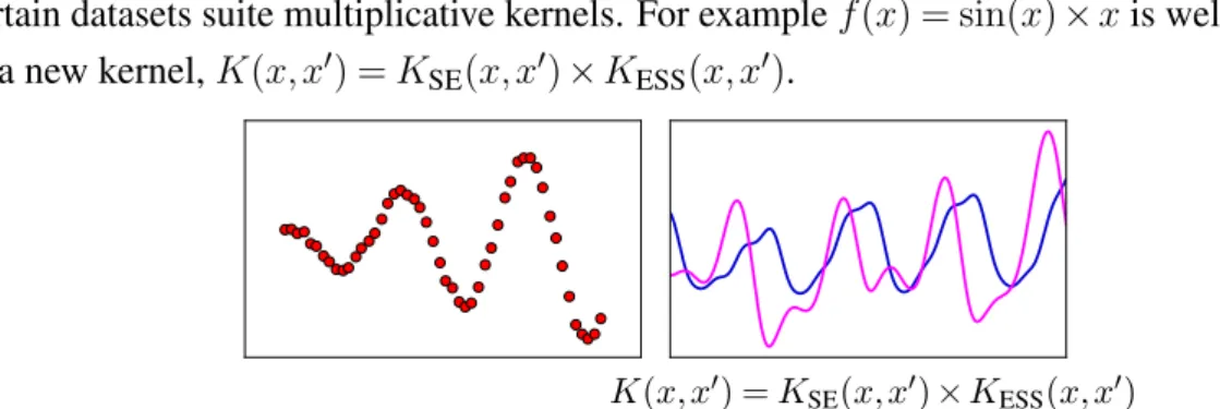
suitable additive kernel combination. . . 32 2.16 Left: Dataset suiting a multiplicative kernel combination. Right: Prior draws
of a suitable multiplicative kernel combination. . . 33 2.17 Prior draws when different kernels are applied to different dimensions of the
input. The right-hand plot uses two SE kernels with differing lengthscales. . 33 3.1 Priors from finite-width BNNs provide an increasingly close approximation
to priors drawn from the equivalent GP kernel when BNN width, H, is increased - here for ERF activation and kernel. . . 42 3.2 Top: Prior draws for infinitely wide single-layer BNNs of various
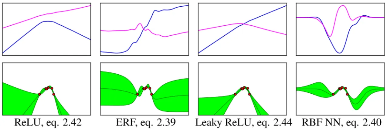
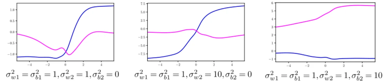
architec-tures. Bottom: Predictive distributions on toy data. . . 43 3.3 Final layer variances: σw22 controls the amplitude of the whole function,
whilstσ2b2controls the spread. ERF activations shown. . . 44 3.4 Final layer variances for classification: σw22controls the both absolute
confi-dence and the speed at which class predictions can switch. Single-layer NN with ReLU activations shown. . . 44 3.5 Prior draws for a single-layer BNN with ERF activations. Increasingσ2w1, σb21
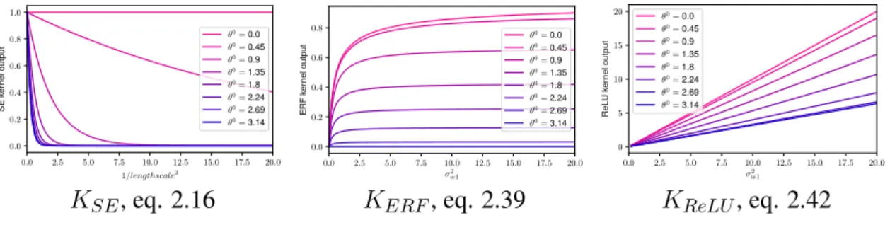
creates noisier functions. Here,σw22= 1, σb22= 0. . . 45 3.6 Kernel analysis, where σ2w2=σb22 and σw22= 1, σb22 = 0. Input angle, θ0
between two inputs is varied whilst the norm,||x||||x′||= 1is held constant. 45 3.7 Prior draws (top & middle: regression, bottom: classification) for finite
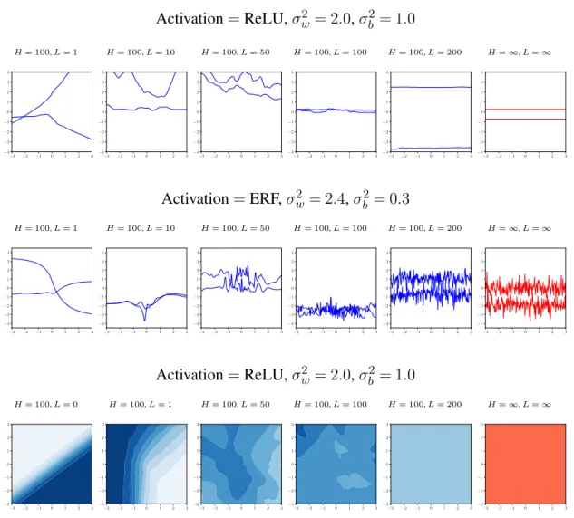
BNNs of increasing depth. These degenerate either into input-independent constants or white noise. In red are prior draws from the ‘infinite’ kernel; that is, by running the recurrence in section 2.6.3 to infinity. . . 46
List of Figures xvii
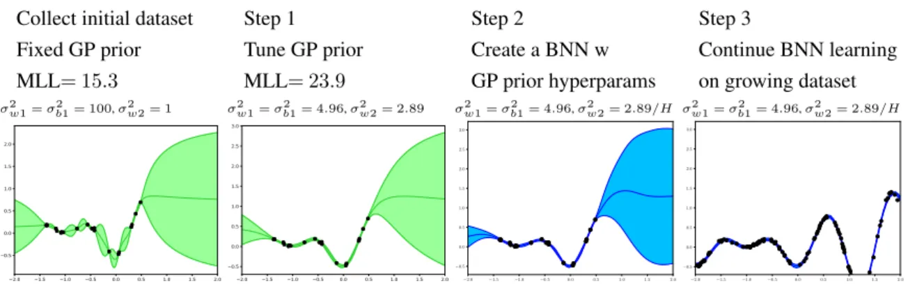
3.8 Using a proxy GP to specify a prior for a single-layer BNN with ERF activations. In step 1, the parameters of the GP ERF kernel (eq. 2.39) are optimised. Note the tuned variance in the GP model is normalised by H
when building the BNN. . . 48 3.9 The cartpole control task is a classic RL problem. Rewards are maximised
by balancing the pole upright. The cart is moved left and right to achieve this, forming the action space for the environment. . . 48 3.10 Performance on a model-based RL task, cartpole, comparing a BNN with
prior tuned using the proposed method (via proxy GP) vs. fixed default prior. Mean±two standard errors, repeated for three runs. . . 49 3.11 BNN architecture determines our prior belief about a function’s properties. In
general BNNs provide little flexibility in this regard - modifying only the ac-tivation function and length scale (‘Basic BNNs’). This chapter explores how to design BNNs to produce more expressive prior functions (‘Combinations of Basic BNNs’). Two prior draws are shown for each BNN architecture. . 50 3.12 Prior draws for a2-Dinput. Square brackets designate which dimension(s)
each kernel is applied to. . . 56 3.13 Two time series with seasonal fluctuations and long term trends. ReLU
and periodic BNNs are separately unable to capture these patterns (first and second from left). However, they succeed when combined in BNN archi-tectures as proposed (third from left), closely approximating the predictive distributions of exact GP inference with the equivalent kernel combinations (right). See main text for model details. . . 60 3.14 Learning for three different BNN architectures on the pendulum task. The
BNN incorporating a suitable prior for task, ‘Periodic×TanH’, outperforms basic BNNs. Mean±1 standard error, three runs. . . 62 3.15 Q-values learnt for the action, torque= 0, conditioned on observations of
˙
θ = 0, and input angle, θ, varied on x-axis and measured in radians. The x-axis range allows observation of three complete rotations of the pendulum (each rotation given by2πradians). Hence, maximum Q-value is predicted when the pendulum is orientated directly upwards. Periodic×TanH captures the local periodicity of the function most accurately. . . 63
4.1 An ensemble of NNs, starting from different initialisations and trained with the proposed modification, produce a predictive distribution approximating that of a GP. This improves with number and width of NNs. . . 67 4.2 Demonstration of (exact) RMS in a 2D parameter space. . . 70 4.3 Examples of the RMS approximate posterior whenµµµanc:=µµµprior,ΣΣΣanc:=
ΣΣΣprior. MFVI also shown. . . 74 4.4 Predictive distributions produced by various inference methods (columns)
with varying activation functions (rows) in single hidden layer NNs on a toy regression task. . . 75 4.5 Empirical plots of conditional likelihoods for 4 randomly sampled parameters
in two-layer NNs. . . 76 4.6 Left: Single layer NN of two hidden nodes. Middle: Draws in parameter
space for prior (red), analytical posterior (blue) and anchored posterior (green). Right: Posterior predictive distribution - dashed red lines are elbows of ReLU units. . . 78 4.7 Comparison of NN ensemble loss choices. . . 79 4.8 The predictive distribution of an anchored ensemble approaches that of a
ReLU GP. . . 80 4.9 Difference in predictive distributions of an anchored ensemble and a ReLU
GP as a function of width and number of NNs. Mean±1 standard error. . . 81 4.10 Anchored ensembling creates uncertainty-aware agents. . . 86 4.11 Anchored ensembling creates robust MBRL agents in noisy environments.
Mean and standard error over five runs. . . 87 5.1 Set up for the toy problem: Left is input data (10 data points linearly spaced
at fixed inputx= 1.0), right is the NN used (one trainable weight). . . 97 5.2 Error surface of LossQD, and LossQDsoft on toy problem, with effect of
hyperparametersλands. . . 98 5.3 Comparison of PI boundaries for GD vs. PSO training methods. Shading
is the predicted 95% PI. Ground truth is given by blue lines - the ideal 95% boundaries and mode. . . 101
List of Figures xix
5.4 Comparison of PI boundaries for two loss functions, QD vs. MVE, given data noise variance drawn from different distributions. Legend as for figure 5.3.102 5.5 Estimation of model uncertainty with a QD ensemble. . . 103 5.6 QD assures global but not pointwise coverage probability. . . 105 5.7 When fitting a single QD NN to uniform data noise, many PIs will give the
same MPIW and PICP. This can lead to diversity in the ensemble, even in regions with much data, and model uncertainty estimates can be overestimated.106 6.1 Qualitative, approximate view of today’s approaches to uncertainty
esti-mation in NNs plotted according to the two criteria targeted in this thesis. Left: The broad classes of techniques. Right: Impact of work in this thesis, comparing the original methods (Deep Ens, LUBE), to the proposals of this thesis (Anch Ens, HQPIs). Circle size roughly represents variability within methods and error of the estimation. . . 112 A.1 Fashion MNIST OOD data examples. . . 156
List of Tables
2.1 Ability of standard NNs to quantify uncertainty types. For regression, it’s assumed prediction is of a single scalar value. . . 20 4.1 NLL regression benchmark results. See appendix A.4 for RMSE (table A.1)
and variants of our method. Mean±1 standard error. . . 82 4.2 Proportion of predictions that were high confidence on out-of-distribution
data, e.g. a single regularised VGG-13 CNN trained on CIFAR-10 made high confidence predictions 54% of the time when asked to predict on MNIST. Mean over five runs (three for CIFAR). ‘Reg.’ refers to standard L2 regularisation, ‘Uncons.’ refers to no regularisation, ‘Anch.’ refers to the proposed anchored regularisation, ‘nxNNs’ refers to an ensemble ofnNNs. 85 5.1 PI quality metrics on ten benchmarking regression datasets; mean ± one
standard error, best result in bold. Best was assessed according to the following criteria. IfP ICP ≥0.95for both, both were best forP ICP, and bestM P IW was given to smallestM P IW. IfP ICP ≥0.95for neither or for only one, largestP ICP was best, andM P IW only assessed if the one with largerP ICP also had smallestM P IW. . . 104 A.1 Variants of our method on benchmark regression datasets, RMSE. Deep
ensembles are included for reference, using published results. . . 151 A.2 Variants of our method on benchmark regression datasets, NLL. . . 151 A.3 Comparison against inference methods on UCI benchmark regression datasets,
log likelihood. Adapted from Mukhoti et al. (2018), also included is the single layer homoskedastic VI results from Tomczak et al. (2018). . . 152
A.4 Fashion MNIST results: proportion of predictions made with≥90% prob-ability, and entropy of predicted categorical distribution. Also shown is relative advantage (percentage change) for each method compared to an-chored ensembles. Averaged over five runs/random seeds, mean±1 standard error. Best result inblue. . . 152 A.5 Hyperparameters used for regression benchmark results. . . 156 B.1 Full permutation results of training method and loss function on synthetic
data with differing noise distributions. Mean±one standard error. . . 163 B.2 RMSE and NLL on ten benchmarking regression datasets; mean ± one
Chapter 1
Introduction
TLDR: Methods for understanding the uncertainty of neural networks are important.
1.1
Big Picture
This thesis contributes to the discipline of building systems that learn from data; machine learning. This promises to deliver flexible, general systems capable of performing tasks requiring some level of cognitive ability. Increasingly, this is referred to under the more grandiose term; artificial intelligence (AI).
AI is beginning to have a major impact on the world. It holds the potential to create new products and services from spam filters to autonomous cars; improve existing ones such as medical diagnosis and language translation; and automate mundane tasks such as production line quality inspection and reading of letter addresses. Projections suggest global GDP could be 14% higher by 2030 as a direct result of AI (Rao and Verweij, 2017).
This thesis focuses on an engineering challenge currently blocking these systems from being more widely applicable in the real-world, and hence unlocking some of this value. It does not focus on a specific application, rather contributing to the fundamental technology that underlies many use cases.
1.2
Breakout Success of Deep Neural Networks
The recent revival of enthusiasm and hope in AI can be put down to the success of a particular class of machine learning model; deep neural networks (NNs). These have proven incredibly effective on specific classes of tasks that traditional approaches struggled with.
Whilst early protoypes of NNs can be traced back as early as 1958 (see section 2.2.1), their value was demonstrated in the 2010s when they were run at scale, training wider, deeper NNs (‘deep learning’), over larger datasets. Notably, these NNs were applied to an image classification task (Russakovsky et al., 2015), delivering a substantial reduction in error rate (Krizhevsky et al., 2012).
As well as a performance improvement, NNs bring an attractive paradigm shift. Previous approaches relied on carefully extracting features using hand-designed rules, followed by a small learnable component. NNs replace this with a single end-to-end learning system. Successes have followed across a variety of vision, audio, control and natural language tasks (Lillicrap et al., 2016; Ping et al., 2018; Radford et al., 2018). NNs have also been combined with the reinforcement learning (RL) framework, creating systems that surpassed human performance in games such as Go, chess, classic 1980s video-games, and modern strategy video-games (Mnih et al., 2015; Silver et al., 2017; Vinyals et al., 2019).
It might appear that this list of achievements could be straightforwardly extended to include any task of interest. However, this overlooks several limitations of today’s NNs. It’s been observed that, ‘it’s easier to build a world champion chess system than it is a mediocre plumber’1. Many sub-fields in machine learning today are, directly or indirectly, developing solutions to these limitations. This thesis is no exception. It contributes to the research effort of building a fundamental property into these systems; that of knowing their uncertainty.
1.3
The Value and Cost of Being Uncertain
The success stories in deep learning to date have been in scenarios where massive datasets were available or could be simulated. ‘Success’ is also in terms of metrics aggregated over a large number of test examples, drawn from the same distribution as the training data. For example, the ImageNet 2015 challenge contained 1.2 million labelled images, with accuracy reported over 0.1 million similar test images (Russakovsky et al., 2015).
This differs in at least two important ways from systems deployed in the real world.
1. Real-world systems do not have guarantees that the data they see when deployed will always be similar to what they were trained on.
2. In real-world systems the confidence inindividual(rather than aggregate) predictions can matter.
1.3 The Value and Cost of Being Uncertain 3
Both these problems are exacerbated by the inability of NNs to properly express their uncertainty.
Regarding point 1), if a system is able to express its uncertainty when presented with an unfamiliar input, there are simple measures that might be implemented, such as referring the case to an expert (a clinician in the example of medical diagnosis), or adopting less risky behaviour (reducing speed in the case of an autonomous vehicle).
To understand point 2), consider a NN predicting the time to failure of a key piece of factory machinery. The system notifies the plant manager that the machine will fail in 60 days. This leaves the manager unsure whether to repair the machine immediately, or if it can be left to run for another 50 days. If the system could communicate its uncertainty with a range this difficulty would be avoided - e.g. 50-70 days with 95% confidence.
In these examples, the value of uncertainty estimates is high. This is in contrast to a typical machine learning benchmark, where classification accuracy might be measured over a large set of test data points, drawn from the same distribution as the training data. Here there is little to be gained from good uncertainty estimates.
As well as there being value to uncertainty estimates, there is also a cost. NNs generally used in practise today are poor at estimating their uncertainty. The techniques reviewed and proposed in this thesis all require modifying these default systems. This brings a cost comprised of two main components; 1) extra implementation effort 2) extra computational requirements. This cost will henceforth be referred to as ‘impact on usability’.
Ideally, one would like uncertainty to have low impact on usability, however, there can be a trade-off between impact on usability and quality of uncertainty estimates. This thesis takes the practical view that methods to quantify the uncertainty of NNs should minimise the impact on usability, whilst producing good quality, or ‘robust’, uncertainty estimates. This is discussed in detail in chapter 6.
1.3.1
Auxiliary Uses
The previous section illustrated the value of uncertainty estimates following deployment of a standard supervised learning system. Aside from this direct use case, uncertainty estimates are valuable in an auxiliary role to many other areas in machine learning. Some of these are listed below.
The most straightforward approach to training NNs requires a large labelled dataset. Whilst for many tasks unlabelled data may be abundant, sourcing labels can be a challenging and
resource-intensive activity. Active learning provides a paradigm for label collection - it allows an algorithm to select which data points it believes it would benefit from being labelled most, hence increasing the efficiency of the labelling process. Having good quality uncertainty estimates available can be important in driving this selection process (Hernández-Lobato and Adams, 2015). This was highlighted as important to Tesla’s efforts in building autonomous vehicles2.
RL describes a learning paradigm where an agent takes actions in an environment, receiving rewards and states. One challenging aspect of this set up is the exploration/exploitation dilemma; at each step the agent must decide whether to exploit its current knowledge, by choosing the action it has observed to be best so far, or explore some new action, which might prove better or worse. Having uncertainty estimates provides agents with an effective approach to handling this dilemma - if the agent is certain an action is optimal, it should exploit its knowledge, whilst if its less certain, it should explore more often (Osband et al., 2016).
These illustrations provide two examples of how uncertainty can be valuable to other sub-fields in machine learning. Other areas that can benefit include adversarial learning (Smith and Gal, 2018), model-based RL (Chua et al., 2018), Bayesian optimisation (Springenberg et al., 2016), meta learning (Finn et al., 2018), continual learning (Nguyen et al., 2018) and behavioural cloning (Menda et al., 2019).
1.4
Research Goal
The previous section motivated the need for uncertainty estimates on the predictions of a NN. This is an active, ongoing research area, and current methods for achieving this, in one way or another, are lacking. This has led to the research goal of this thesis.
Research Goal
Develop techniques enabling NNs to communicaterobust uncertainty estimates on their predictions, whilst minimisingimpact on usability.
‘Impact on usability’ was previously defined. The research goal also places emphasis on the uncertainty estimates being useful and reliable - here termed ‘robust’, due to common usage in the field. In simple terms, the goal states the uncertainty estimates be of maximal value and minimal cost.
1.5 Contributions 5
There are numerous directions worthy of exploration with this goal in mind. Of the various existing techniques (section 2.3), each has advantages warranting further analysis, and disadvantages warranting modification.
This thesis has chosen to drill down into several distinct areas within the research goal that are of high importance to the field. Each investigation will be presented separately, since they study slightly different perspectives on the same goal, and their effectiveness is most easily demonstrated in isolation. However, it should be noted that they are not necessarily mutually exclusive ideas. Chapter 6 provides a framework to visualise the value produced by the contributions of the thesis.
1.5
Contributions
One of the recurring themes in this thesis is the distinction between Bayesian vs. non-Bayesian methods. The non-Bayesian framework gives a rigorous and widely accepted approach to handling uncertainty in any predictive model. As such, it is one of the most important approaches to handling uncertainty with NNs.
One challenge of the Bayesian approach in NNs, is that it is not obvious how to specify parameter priors that capture appropriate prior knowledge about a task. The first contribution of the thesis is both a practical tool to do this, and a lens to understand the meaning of parameter priors.
Contribution 1- Expressive Priors for Bayesian NNs, Chapter 3
This chapter proposes to use the link between GPs and NNs to design better priors for Bayesian NNs. The link allows conversion of a functional prior (in a GP) to a parameter prior (in a Bayesian NN). The main contribution then shows how a popular idea for prior design in GPs (kernel combinations) can be translated to Bayesian NNs.
A second challenge of Bayesian NNs is how to efficiently learn the posterior parameter distribution. Indeed a large proportion of the literature in Bayesian NNs focuses on this. Stochastic gradient descent (SGD) is effective in optimising deterministic NNs, but it is not straightforward to apply this to the setting where parameters are modelled as distributions. On the other hand, ensembles of NNs do use SGD and provide a practical way of computing uncertainty estimates - a number of independent NNs are trained with SGD, and the variance of their predictions is interpreted as uncertainty. Our second contribution reconciles these two approaches.
Contribution 2- Bayesian Ensembling, Chapter 4
Ensembles of NNs have often been shown to outperform Bayesian methods, though are sometimes criticised for lacking a rigorous theoretical framework. This has led to a difficult choice; select the ad-hoc method that works well empirically, or use the more theoretically grounded method. The chapter introduces a third alternative; a modified ensembling procedure that does have strong to connections to the Bayesian framework. Combining these two paradigms results in performance superior to vanilla ensembling.
The third contribution of the thesis moves away from Bayesian methods and considers a NN with two outputs representing the upper and lower bounds of a prediction interval (PI). This makes for an interesting contrast with earlier contributions in Bayesian methods. On the plus side, the intuitive NN architecture and loss function provide a transparent and directly interpretable set up. On the downside, we document a failure mode of the method, providing an exemplum of the potential perils of non-Bayesian methods.
Contribution 3- High-Quality Prediction Intervals, Chapter 5
Adopting the axiom that PIs should be as narrow as possible subject to a certain coverage proportion, this chapter proposes a carefully designed objective function that can be used with SGD. This holds a significant advantage over previous work, which was not compatible with SGD. The chapter also shows that previous work failed to capture one source of uncertainty entirely, and proposes combining with a (vanilla) ensemble to address this.
1.6
Thesis Structure
The following is an overview of the thesis structure.
Chapter 1provides a high-level overview of deep learning, and motivates the need for NNs to be able to estimate their uncertainty. The goals, contributions and structure of the thesis are communicated.
Chapter 2provides prerequisite knowledge to understand later contributions. The following topics are introduced: uncertainty modelling, NNs, uncertainty modelling with NNs, BNNs, GPs, and the connection between BNNs and GPs. The chapter serves as a broad literature
1.7 Publication List 7
review for the thesis, though each technical chapter also contains a focused related work section.
Chapter 3presents the first technical contribution of the thesis, which helps specify appropri-ate priors for BNNs. Broadly, the chapter utilises the link between GPs and BNNs to provide a lens to study the effect of parameter priors in a NN on functions. Most significantly, it translates a popular idea for prior design in GPs (kernel combinations) to BNN architectures for the first time. It draws from publications (Pearce et al., 2020b, 2019b; Tsuchida et al., 2020).
Chapter 4studies a modified version of ensembling NNs; parameters are regularised around a random draw from the prior. The chapter shows this provides connections to a little-known Bayesian inference technique, ‘randomised MAP sampling’. Novel theoretical results as well as empirical experiments are offered. This forms the thesis’s second contribution and draws from publications (Pearce et al., 2018a, 2019a).
Chapter 5derives a loss function allowing a NN to directly output PIs, and shows how it can be made compatible with gradient descent. An explanation for why it should be used together with ensembling is also given. The related publication is (Pearce et al., 2018b).
Chapter 6firstly summarises the contributions of the thesis, and lists follow up work already completed by other authors. The current field is visualised by plotting existing methods on two axes; robustness of uncertainty estimates and impact on usability. We detail the impact of the contributions of this thesis. The chapter then takes a more speculative view of the future of uncertainty in AI. Drawing from (Pearce et al., 2020a), it argues for exploring new paradigms for uncertainty quantification as AI systems grow ever larger and more general. Finally, directions for future work generated throughout the thesis are curated.
1.7
Publication List
The following publications, preprints and extended abstracts were produced over the course of the PhD. Unless stated, the first author of the paper was responsible for the vast majority of technical work.
• AS Palau, K Bakliwal, MH Dhada,T Pearce, AK Parlikad
IEEE International Conference on Prognostics and Health Management 2018 - T Pearce contributed to the implementation and tuning of the RNN.
• T Pearce, M Zaki, A Brintrup, A Neely
High-Quality Prediction Intervals for Deep Learning: A Distribution-Free, Ensembled Approach
ICML 2018
• T Pearce, R Tsuchida, M Zaki, A Brintrup, A Neely
Expressive Priors in Bayesian Neural Networks: Kernel Combinations and Periodic Functions
UAI 2019
• R Tsuchida,T Pearce, C Van Der Heide, F Roosta, M Gallagher
Avoiding Kernel Fixed Points: Computing with ELU and GELU Infinite Networks AAAI 2020
- T Pearce set up the GELU kernel derivation, and ran the benchmarking regression experiments.
• T Pearce, N Anastassacos, M Zaki, A Neely
Bayesian Inference with Anchored Ensembles of Neural Networks, and Application to Exploration in Reinforcement Learning
Exploration in Reinforcement Learning Workshop, ICML 2018 • T Pearce, F Leibfried, M Zaki, A Brintrup, A Neely
Uncertainty in Neural Networks: Approximately Bayesian Ensembling AISTATS 2020
• T Pearce, A Brintrup, A Neely
A Neuroscience-inspired Approach to Building Uncertainty-aware AI NAISys 2020
• T Pearce, A Y K Foong, A Brintrup
Structured Weight Priors for Convolutional Neural Networks
Chapter 2
Background
TLDR: Prerequisite reading for the thesis; uncertainty, neural nets, Bayesian neural nets, Gaussian processes.
This chapter introduces elements important to the broad theme of this thesis: modelling uncertainty with NNs. This is prerequisite knowledge for understanding the contributions presented later in the thesis.
• Section 2.1 - An explanation of the types of uncertainty typically defined in statistical modelling, and how they arise in regression and classification.
• Section 2.2 - Introduces the core model of this thesis: NNs. This is done through a biological lens, which sets up the closing discussion in chapter 6.
• Section 2.3 - Briefly reviews several existing methods which allow NNs to model uncertainty. Chapter 5 will contribute a new method.
• Section 2.4 - A more detailed look at one of the leading methods for modelling uncertainty in NNs: Bayesian NNs. Chapters 3 to 4 contribute in this area.
• Section 2.5 & 2.6 - GPs are naturally able to capture uncertainty. We review this model and describe connections to BNNs. Chapter 3’s contributions build on this.
This chapter serves as both a technical primer and macro-literature review with key literature sources being cited. Each technical chapter (3, 4, 5) further contains a focused literature review relevant to the specific contribution.
2.1
Anatomy of Uncertainty
Consider building a model to predict a person’s height given their age, sex and race, using a dataset of thousands of people living in a small town in Cambridgeshire, UK. The model is then asked to make height predictions for two people.
1. A Caucasian male of 43 years.
2. An aboriginal Taiwanese male of 21 years.
Based on the dataset, the height range for the first might be given as falling between 5’8" to 6’2". The second one is more difficult, since the dataset may not contain any instances of aboriginal Taiwanese. To be cautious, the model might want to output a greater range of 5’6" to 6’5".
The range on the two answers communicates that there is uncertainty in both, but thetype of uncertaintyis different. The first is uncertainty due to factors outside of one’s model of the task (‘aleatoric uncertainty’), the second is additionally uncertain due to lack of knowledge (‘epistemic uncertainty’) (Der Kiureghian and Ditlevsen, 2008).
In general, epistemic uncertainty can be reduced by collecting more data on a task (here, one could collect heights of Taiwanese natives). Aleatoric uncertainty cannot, though it might be reduced by collecting additional information about new variables (here perhaps the weight of the individual).
It’s important to note that this aleatoric/epistemic distinction is a consequence of modelling choices, and is not some absoluteproperty of the task. For example, if instead of using a dataset collected in the Cambridgeshire town, it was collected in Taitung county, the epistemic assignation would be reversed.
A brief philosophical note
Typically, the uncertainty on the outcome of a roll of a dice might be thought of as aleatoric. But is it really? The outcome is some predictable function of release angles, momentum, friction coefficients and so on. In which case why not call it epistemic? Hence, we argue it is more of a modelling choice. Thinking more deeply about the difference between aleatoric and epistemic uncertainty can lead to interesting questions: Is the world inherently stochastic? Does randomness truly exist?
2.1 Anatomy of Uncertainty 11
x
y
x x
Figure 2.1 Visualising aleatoric uncertainty. Even with a large amount of data, uncertainty may remain. Left: Low homoskedastic noise. Middle: High homoskedastic noise. Right: Heteroskedastic noise.
2.1.1
Regression
We now consider, more formally, these two sources of uncertainty in regression tasks, where we predict some scalar,y∈R, based on some inputx∈Rd. Generally it is not possible to perfectlypredict the valuey, since the input features do not contain every detail required. As such, we often assume a model with additive noise,ϵ,
y=f(x) +ϵ. (2.1)
Following from above, ymight represent a person’s height, whilstxis information about their age, sex and race. Knowing these xvariables is not enough to perfectly predict a person’s height, hence we model this unknown with a random variable,ϵ. This represents the
aleatoricuncertainty.
Homoskedastic vs. Heteroskedastic Aleatoric Uncertainty
A simple, practical choice for this random variable is,ϵ∼ N(0, σϵ2), whereσ2ϵ is a parameter to be estimated. This implies thatϵdoes not depend onx, which is known ashomoskedastic
noise. Alternatively, one could define and learn a new function that is dependent on the data,fϵ(x), which leads toheteroskedasticnoise,ϵ∼ N(0, fϵ(x)). An example of each is
visualised in figure 2.1.
Epistemic Uncertainty
We now consider epistemic uncertainty. Our ultimate goal is to capture the uncertainty ofy
4 2 0 2 4
x
y
4 2 0 2 4
x
Figure 2.2 Visualising epistemic uncertainty. Left: A prediction ofywhenx= 0.5should be more certain than whenx= 4.0. Right: Uncertainty inf(x)increases further from the training data.
xandy, we have,
y=f(x) +ϵ
Var[y] =Var[f(x) +ϵ]
=Var[f(x)] +Var[ϵ] (2.2)
Total Uncertainty=Epistemic+Aleatoric.
As discussed,Var[ϵ]is estimated as part of the model - by learningfϵ(x)orσ2ϵ. From eq. 2.2
we see we also need to estimateVar[f(x)], which is the estimated variance of the function. Indeed, this uncertainty overf(x)is our epistemic uncertainty. Typically a model might learnf(x)for some region of the input space covered by the training data, but there will be regions outside of that which it will be uncertain about. This is visualised in figure 2.2.
2.1.2
Classification
The previous two types of uncertainty also apply to classification tasks. Consider a binary classification task, with two possible classes,y∈ {c1, c2}. Figure 2.3 shows a simple 1-D set
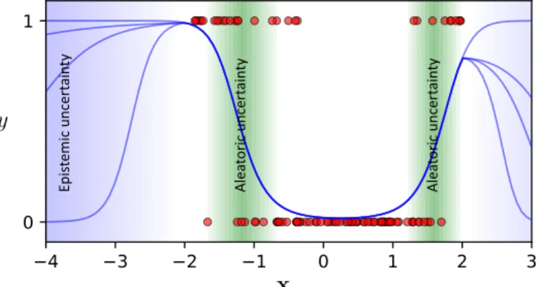
up. Whenx= 0, we can confidently sayP(y= 1)≈0.0. Whenx=−1.2, we can equally sayP(y= 1)≈0.5. Although we are unsure of the class prediction here, we are quite sure that it is0.5. This uncertainty arises from inherent noise in the data and is aleatoric. On the other hand, if asked to predict atx=−4, we might again sayP(y= 1)≈0.5, but this time uncertainty derives from having no data in this region of the input space, and hence little knowledge about the underlying function, so our uncertainty and is epistemic.
2.2 Neural Networks 13 Ep ist em ic u nc er tain ty Al ea to ric unce rt ai nt y Al ea to ric unce rt ai nt y x y
Figure 2.3 1-D binary classification task showing two sources of uncertainty. Blue lines show plausible estimates forPˆ(y=c1|x). The multiple lines arise from uncertainty inf(x).
2.1.3
Other Uncertainties
Above, we have introduced the two sources of uncertainty we will model through this thesis. Care must be taken as these sources appear under various names. Aleatoric uncertainty may be referred to as irreducible noise, data uncertainty, data noise, or known unknowns. Epistemic uncertainty as model uncertainty, or parameter uncertainty.
More confusingly, sometimes the two sources are decomposed or slightly redefined. For example, Lakshminarayanan et al. (2017) talk about calibration (which is related to aleatoric uncertainty) and domain shift / out-of-distribution (OOD) uncertainty (which is related to epistemic uncertainty). Malinin & Gales (2018) explicitly introduce a further source: distributional uncertainty, which allows their proposed model to distinctly model aleatoric and OOD uncertainty, both in a maximum likelihood fashion. They note that this is implicitly covered by epistemic uncertainty under the Bayesian framework.
Finally we note that other types of uncertainty exist that are not considered in this thesis. For example, input uncertainty, where there is uncertainty on the input values.
2.2
Neural Networks
This section provides a primer on NNs. Historically, there have been two broad approaches to building AI systems.
1. Symbolic AI (also ‘expert systems’, ‘Good Old-Fashioned Artificial Intelligence’) takes the view that thought is the manipulation of symbols (words, concepts). Encoding
Figure 2.4 Left: Modern diagram of a single neuron. Right: Early sketches of neuons based on thin slices of brain tissue by Ramón y Cajal.
knowledge into a system, operated on by the rules of logic, may lead to an intelligent system.
2. Connectionism takes an alternative view; that intelligence might emerge through simulating the hardware of a biologically intelligent system.
This second view was the original motivation for building artificial NNs. Whilst today the field of machine learning is quite separate from these biological origins, we use the analogy to provide an intuitive introduction to NNs. This connection also motivates our discussion in section 6.
2.2.1
Origins: Modelling Biological Neurons
In 1888, Ramón y Cajal published evidence that the brain consisted of networks of individual neurons (figure 2.4) (López-Muñoz et al., 2006). This marked the birth of the idea that networks of neurons provide the basis of intelligence.
The first major work on the computational modelling of these networks was published in 1943 by McCulloch & Pitts (1943), when it was put forward that neurons with binary activation functions could do first order logic.
The nervous system is a net of neurons, each having a soma and an axon. Their ... synapses are always between the axon of one neuron and the soma of another. At any instant a neuron has some threshold, which excitation must exceed to
2.2 Neural Networks 15
Figure 2.5 Diagram of an early perceptron by Rosenblatt (1958).
initiate an impulse... From the point of excitation the impulse is propagated to all parts of the neuron.
McCulloch & Pitts (1943)
The idea of synaptic weights being the basis of learning was then developed by Hebb (1950), captured by the well known phrase:cells that fire together wire together. In 1958, Rosenblatt combined this idea with that of McCulloch & Pitts, proposing a computational model of a neuron with learnable weights (Rosenblatt, 1958). This is perhaps the earliest recognisable relative of modern day NNs (figure 2.5).
2.2.2
From Neurons to Deep Neural Networks
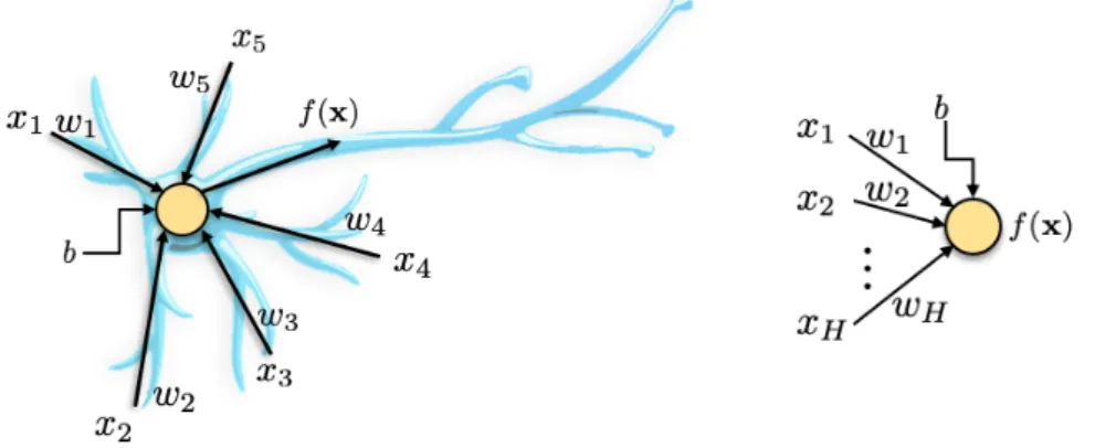
NeuronsFigure 2.6 (left) shows a diagram of a biological neuron, withxirepresenting input signals
into the neuron,withe synaptic weights,bsome bias it must overcome in order to fire, and
f(x)the output. On the right the figure shows the computational graph of an artificial neuron. Biological neurons outputspikesof action potential which vary over the temporal dimension. Conversely, artificial neurons output a continuous value and do not operate over a temporal dimension. The most plausible way to connect these two models is to interpret artificial neurons as modelling therateat which spikes are being fired (firing rate) in the biological neuron given some steady stimulus (Pfeiffer and Pfeil, 2018).
The equation governing the output of an artificial neuron is given by,
f(x) =ψ H X i=1 wixi+b ! (2.3) =ψ(w⊤x+b) (2.4)
Figure 2.6 Diagram of a single neuron. Left: Overlaid on biological neuron. Right: Ab-stracted computational graph.
for some activation function, ψ, input x∈RH, weight vector,w∈RH, bias b∈R, and outputf(x)∈R. This thesis will tend to use vector and matrix notation in eq. 2.4.
It might be hard to see how eq. 2.4 will be of interest. Whilst each neuron carries out a simple operation, by connecting these neurons into large structured networks, powerful computational mappings can be built.
Single Layer Neural Networks
We now build a simple single layer NN composed of artificial neurons. Figure 2.7 shows a NN with a single input and output neuron andH hidden neurons.
Figure 2.7 Single-layer NN (biases not drawn for clarity).
The output of the NN with a general number of inputs (d) and outputs (dout) is computed,
f(x) =b2+W2ψ(W1x+b1), (2.5)
whereW1∈RH×d, andb1∈RH, whilstW2∈Rdout×H andb2∈Rdout. The activation,ψ,
2.2 Neural Networks 17
Deep Neural Networks
If wide enough, single layer NNs are able to approximate any function (Debao, 1993). However, it’s been argued that adding layers, rather than width, produces models better suited to the types of task typically encountered (Bengio, 2009; Poggio et al., 2017). The arguments are non-trivial, describing depth as important to learn compositional, or highly-varying functions, which it is argued are properties of vision and language. The empirical success of deep models provides evidence for this, and it is from their effectiveness that the term ‘deep learning’ emerged (Goodfellow et al., 2016). Figure 2.8 shows a NN with three hidden
layers. Computations are as before, but now must be performed recursively as in eq. 2.6.
Figure 2.8 Deep NN with three hidden layers.
fL(x) =bL−1+WL−1ψL−1 fL−1(x)
(2.6) Where the dimensions ofWL−1andbL−1depend on the number of neurons in the adjacent
layers.
Complex Architectures
So far we have considered fully-connected NNs, where neurons are organised into layers, and each neuron in a layer is connected to every neuron in the adjacent layers. This is a somewhat arbitrary choice of connectivity, and a variety of alternatives exist. Figure 2.9 contains illustrations of three: autoencoders, recurrent NNs, and convolutional NNs. Much of deep learning’s success derives from using architectures suited to a task (often termed ‘structural priors’) (Goodfellow et al., 2016).
Amongst the most important of these architectures, and of most relevance to later experiments in this thesis, is the convolutional NN (CNN), which can be viewed as a sparsely-connected NN with weight sharing. This encourages translational equivariance - a feature produces similar output regardless of it’s local position in the input - and makes it particularly suitable
Figure 2.9 NNs with various connectivity patterns. Left: Autoencoder. Middle: Recurrent NN. Right: CNN.
for data with a spatial or temporal aspect, such as images. The CNN was originally designed to mimic the wiring pattern in human visual systems (Hassabis et al., 2017).
2.2.3
Learning in NNs
Learning in biological intelligence involves modifying synaptic weights of a biological NN. Until now, we have discussed only the structure and computations carried out by artificial NNs in order to get from input to output, and assumed the weights and biases (parameters) are given. Goodfellow et al. (2016) provides a reference for this section.
In order for a NN to be useful, it is necessary to specify parameter values that perform a desired input-output mapping. The process through which these parameters are specified is known as learning or training. One of the major challenges in NNs has been developing effective methods for doing this.
Generally, it is framed as an optimisation problem. A cost function (also ‘loss function’ or ‘objective function’) is defined based on the desired outcome of the task. In a supervised
regression setting, this might be,
Lθ(θ,x,y) = 1 N N X i=1 (yi−yˆi)2, (2.7)
whereyˆi=f(xi, θ)is the output of the NN,θare the NN parameters, andxiandyirefers to
theith input and output respectively.
The optimisation problem is to minimise the cost function by adjusting the parameters. This is commonly done using gradient descent, which uses the partial derivative, ∂θ∂L
2.3 Modelling Uncertainty with Neural Networks 19
loss changes given a (infinitesimally) small increase inθi. The update rule is then,
θi,t+1=θi,t−τ
∂L ∂θi,t
, (2.8)
at learning stept, for some learning rate,τ, controlling the size of the update. Rather than computing the gradient over the whole dataset, in practice it is often computed over some subset (‘mini-batch’) of the data. This introduces some noise to the update step, hence the learning process is termed stochastic gradient descent (SGD). In order to compute the term ∂θ∂L
i for all parameters in the NN, backpropogation is used, which applies the chain
rule successively backwards through the NN. In order to calculate the derivatives, the loss function and NN operations must be differentiable.
Eq. 2.8 gives the vanilla gradient descent update rule. Modern NNs often use variants such as Adam (Kingma and Ba, 2015), which stores a moving average of the gradient mean and variance, and allows more effective weight updates to be made.
2.3
Modelling Uncertainty with Neural Networks
Having introduced uncertainty in section 2.1 and NNs in section 2.2, this section details the ability of standard NNs to model uncertainty. They are found lacking in certain areas, and the section proceeds by summarising existing methods and modifications that can improve their ability to model uncertainty.
A new method is contributed in chapter 5, and improvements to one of the most promising approaches are made in chapters 3 and 4.
2.3.1
Can Standard Neural Networks Model Uncertainty?
Can standard NNs (defined as in section 2.2) used for regression and classification tasks com-municate an appropriate level of epistemic and aleatoric uncertainty relating to a particular prediction? Table 2.1 summarises the answer.
By using a NN to parameterise a probability distribution, aleatoric uncertainty can be captured. For a classification NN, outputs can be squashed through a softmax, creating a final output that can then be interpreted as a multinomial distribution. A regression NN with one output could represent the mean of a normal distribution, with constant variance, capable of capturing only homoskedastic noise. A second output could be added to represent an
Table 2.1 Ability of standard NNs to quantify uncertainty types. For regression, it’s assumed prediction is of a single scalar value.
Classification NN Regression NN Regression NN (one output) (two outputs)
Aleatoric (Homoskedastic) ✓ ✓ ✓
Aleatoric (Heteroskedastic) ✓ ✗ ✓
Epistemic ✗ ✗ ✗
input-dependent variance, which would capture heteroskedastic noise. (Note that the loss function must be matched to the architecture.) These set ups are further detailed in section 2.4.1.
When asked to predict on a data point unlike the training data, the NN should increase its uncertainty. There is no mechanism built into standard NNs to do this. Even in the case of a two-output regression NN, there is no reason for the estimated variance to increase for a new data point. As such, standard NNs cannot estimate epistemic uncertainty. This is unfortunate since epistemic uncertainty is often the more useful component of the two; it is required for many use cases described in chapter 1, such as active learning, exploration in RL, and knowing when an unusual input is received.
2.3.2
Overview of Methods
This section briefly introduces some common methods used to improve uncertainty estimates of NNs.
Quantile Regression
Eq. 2.7 details a loss function that trains a NN to estimate the mean of a scalar target. Using instead,P
|yi−yˆi|, encourages output of the median. Further modifying to,τP∀yi<yˆi(yi−
ˆ
yi) + (τ−1)P∀yi≥yˆi(yi−yˆi), encourages return of some quantile (theτ percentile) of the
predictive distribution (Koenker and Hallock, 2001; Taylor, 2000). Note that no distributional form has been assumed. By estimating, say the0.025and0.975quantiles, a 95% PI could be constructed. Quantile regression is only able to capture aleatoric uncertainty.
2.3 Modelling Uncertainty with Neural Networks 21
Conformal Prediction
This method uses previously seen data to determine prediction regions (e.g. a prediction interval) that provide coverage with some pre-set probability (Shafer and Vovk, 2008). The size of the region indicates the uncertainty. Usefully, it is compatible with any predictive model, including NNs. It is difficult to determine the link with aleatoric and epistemic uncertainty (Hüllermeier and Waegeman, 2019).
Ensembling
A simple approach to estimating uncertainty is to train a small number of NNs (an ensemble), beginning from different initialisations and sometimes on noisy versions of the training data. When asked to make predictions on new data, there will be some diversity in the ensemble’s predictions, which can be interpreted as the uncertainty. The intuition is simple: if the new data point is similar to the training data, the NNs should all produce similar estimates, but if it is very different, there should be higher variance in the predictions.
This is generally presented as a non-Bayesian alternative to epistemic uncertainty estimation (Lakshminarayanan et al., 2017). Chapter 4 discusses this claim more thoroughly, and presents a modification that does lead to strong connections to Bayesian methodology.
Prior Networks
This recently proposed approach explicitly trains a NN to be uncertain on OOD data (Malinin and Gales, 2018). These OOD samples are generated either through adversarial techniques, or by using alternative datasets (e.g. train on CIFAR and use SVHN as OOD examples). This is most useful when these samples are representative of OOD data that will be encountered in the real world. The result is a single NN with good resistance to OOD examples. On the other hand, it may not be straightforward to extend the method to use cases of BNNs such as exploration and active learning, where the training distribution is incrementally growing. Prior networks can capture both aleatoric and epistemic uncertainty.
Bayesian Neural Networks
The Bayesian framework provides a principled framework for handling uncertainty, and has been combined with numerous models and applications. At its simplest, it specifies how to update beliefs (e.g. about functions) in light of evidence (e.g. data points), in an optimal
fashion. It was first applied to NNs in 1992 (MacKay, 1992b), motivated as a principled way to do hyperparameter selection as well as for its ability to capture epistemic uncertainty. A large body of work has followed, more recently under the name ‘Bayesian deep learning’. It is arguably the most prominent approach to handling uncertainty in NNs (as an example, the Baysian Deep Learning workshop has attracted around 100 abstracts in recent years at the NeurIPS conference, bayesiandeeplearning.org). The contributions of this thesis are primarily in this area, as such the following section fully introduces these models.
2.4
Making Neural Networks Bayesian
2.4.1
Distributions Over Parameters
Earlier we introduced weights of a NN as scalar numerical values, that represent the strength of a connection between two neurons, and can be learnt using gradient descent.
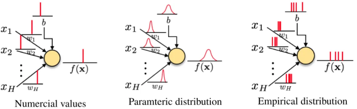
A Bayesian NN requires a conceptually different set up. Rather than assigning each parameter a specific numerical value, we will instead model them as random variables with a probability distribution. This could either be a parametric probability distribution (such as normal or uniform), or an empirical probability distribution (by storing a set of parameter samples). Figure 2.10 illustrates this. Note that probability distributions are shown as though parameters are independent of each other, though this need not be the case.
Probability distributions in general are used to describe the uncertainty over the value of some variable, and this is no exception: we use them to represent the uncertainty in parameters.
Numercial values Paramteric distribution Empirical distribution
Figure 2.10 A neuron with point estimates over parameters produces a point estimate at its output. If parameters are modelled with distributions (parametric or empirical), the output will also be a distribution.
2.4 Making Neural Networks Bayesian 23
Although relatively straightforward conceptually, this new set up has implications both for computing the feedforward output (how should the output of the BNN now be com-puted?), and more challenging, the learning process (how can gradient descent be applied to distributions?).
Bayesian Posterior Distribution
Assigning arbitrary distributions to parameters doesn’t make a NN Bayesian. Bayesian NNs mean a NN with a specific distribution over the parameters, this distribution is known as the ‘Bayesian posterior’, denotedP(θθθ|D). Here,D, stands for some dataset, which in supervised learning is a set of input/output pairs,D={(x1,y1),(x2,y2), . . . ,(xn,yn)}. It is simple to
write an equation to calculate this posterior distribution in terms of several other distributions.
P(θθθ|D) = P(D|θθθ)P(θθθ)
P(D) (2.9)
Note that we have slightly abused notation here, and more precisely can be written,P(D|θθθ) :=
P({yi}ni=1|θθθ,{xi}ni=1), and,P(D) :=P({yi}ni=1|{xi}ni=1).
Likelihood
On the RHS of eq. 2.9 is,P(D|θθθ), called the ‘likelihood’, which represents how likely the data is given the parameters. It returns a single scalar representing the probability of drawing that dataset, given the model parameters.
In order to formulate the likelihood function some probability distribution is specified that is parameterised by the output of a NN. For a regression task a NN with a single output might specify the mean of a normal distribution, with constant variance. If data points are treated independent and identically distributed (iid), the likelihood is then given by,
P(D|θθθ) =
N
Y
i=1
N(yi|f(xi,θθθ), σϵ2), (2.10)
where the NN prediction has been written,f(x,θθθ), to explicitly depend on the parameters, and some amount of noise has been assumed in the data, of varianceσ2ϵ. This is appropriate if the data noise is homoskedastic (section 2.1.1).
If there is reason to believe the data noise is heteroskedastic (section 2.1.1), one might use a NN with two outputs, one specifying the mean and one the variance (or log variance to
ensure it’s positive). The likelihood is then, P(D|θθθ) = N Y i=1 N(yi|f1(xi,θθθ), f2(xi,θθθ)). (2.11)
For classification tasks, withCclasses, and one-hot-encoded labelsyi,j ∈ {0,1}, it’s usual to
have a NN withCoutputs, which are passed through a softmax function in order to convert into a normalised probability (each output between0and1, together sum to1). Denoting
fj(xi,θθθ)as outputj after the softmax, the likelihood is given by a multinomial distribution,
P(D|θθθ)∝ N Y i=1 C Y j=1 fj(xi,θθθ)yi,j. (2.12)
This covers the likelihood functions most commonly implemented with BNNs.
Prior
Also in eq. 2.9, we have,P(θθθ), which is termed the ‘prior’. Broadly speaking, a modeller sets this distribution based on prior knowledge available about the task.
Textbook introductions to Bayes might give examples about coin flipping, where a parameter represents the probability of a coin being biased. The prior encodes an initial belief about this parameter, which is updated by observed data. NNs introduce a complication; it is not obvious what a prior distribution over a NN parameter means about the implied prediction, which is what a modeller might have knowledge about.
It is common (though by no means necessary, e.g. (Nalisnick, 2018)) for BNNs to have iid Gaussian priors, of constant mean and variance across a layer, which leads to interesting connections with GPs. This connection forms an important foundation for later contributions, and is described in section 2.6. This will allow an interpretation of parameter priors as functional priors.
A prior is generally set before observing evidence, however empirical Bayes describes a paradigm whereby hyperparameters controlling the prior are set to be their most likely values according to the data. For example, in a GP this could be the kernel length scale, or in BNNs, the variance of the weight priors for a particular layer. Note that this philosophy faces some criticism (Blundell et al., 2015; Gelman, 2008).
2.4 Making Neural Networks Bayesian 25
Marginal Likelihood
The final term on the RHS of eq. 2.9 is P(D), known as the ‘marginal likelihood’ or ‘evidence’ or ‘prior predictive distribution’, calculated by,
P(D) =
Z
P(D|θθθ)P(θθθ)dθθθ. (2.13) A simple interpretation is that it is a normalising constant, ensuring thatP(D|θθθ)P(θθθ)sums to one over the domain ofθθθ, which is a requirement of a probability distribution.
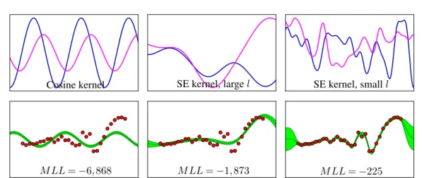
It is also useful as a measure of how well a model fits the data (Rasmussen and Williams, 2006). This can be valuable in empirical Bayes procedures where hyperparameters of the prior are to be estimated. Examples of this are provided for a GP in figure 2.14.
2.4.2
Posterior Predictive Distribution
In models where parameters themselves are of interest (as in the coin flipping example), it might be that generating their posterior probability distribution, P(θθθ|D), is the goal of Bayesian inference. By contrast, in NNs we are less interested in the parameter distributions themselves, and more interested in making predictions using the posterior distributionP(θθθ|D)
for some new data point,x∗. This leads to the posterior predictive distribution,P(y∗|x∗,D).
P(y∗|x∗,D) =
Z
P(y∗|x∗,θθθ)P(θθθ|D)dθθθ (2.14) One insight used in later contributions (chapter 4) is that provided samples can be generated from the posterior, it may not be necessary to fully capture the parameter posterior itself.
2.4.3
Learning in BNNs
In section 2.4.3, we described a learning mechanism, SGD, which is widely used for NNs with point estimates of the parameters and a defined loss function. One of the major challenges of BNNs is that we can no longer use this mechanism directly. The objective of BNNs is to find the posterior distribution; but there is no obvious loss function that can be minimised, nor is it clear how the parameter update rule in eq. 2.8 would apply to distributions.
Computing the posterior analytically is possible only in special models where the prior and likelihood distributions are conjugate. This occurs, for example, with a beta prior and
Bernoulli likelihood, which apply in the coin flipping example. For most models, including BNNs, eq. 2.9 is not tractable.
We now briefly introduce the main classes of techniques used to perform Bayesian inference in NNs. Note that this is an vast, active area of research and we attempt to summarise only the main approaches.
One of the disadvantages of many of these methods is that they fall outside common frame-works used for training NNs used by the majority of the community. Indeed one method that doesn’t, MC Dropout, is (arguably) the most widely used because of this. Our proposal in chapter 4 provides a similarly easy-to-implement method.
Sampling Methods - MCMC, HMC
Markov chain Monte Carlo (MCMC) methods provide a procedure for sampling from a probability distribution. Stochastic chains explore the parameter space. They are designed so that the stationary distribution of the chain matches the target probability distribution. Hence one can obtain a set of parameter samples forming an empirical distribution.
MCMC methods can be implemented with a variety of algorithms. Metropolis–Hastings works well in smalls-scale settings but can be slow to converge for more complex scenarios. Hamiltonian Monte Carlo (HMC) uses gradient information to move around the parameter space more efficiently. It was shown to be better suited to use in BNNs (Neal, 1997), and more recently has been made more practical (Chen et al., 2014).
Variational Inference
Variational inference (VI) provides an alternative paradigm to sampling methods. A para-metric approximating distribution is defined, qν(θθθ), with the goal of finding distribution
parameters, ν, to minimise the Kullback–Leibler divergence between the approximating distribution and the true posterior, argminν DKL(qν(θθθ)||p(θθθ|D)). This optimisation is done
by maximising a surrogate quantity called the ELBO (evidence lower bound), given by, ELBO=
Z
qν(θθθ) logp(D|θθθ)dθθθ+KL(qν(θθθ)||p(θθθ)) (2.15)
The major attraction of the method is precisely that it can be framed as an optimisation problem, which opens the door to widely used tools already available. A disadvantage is that the the quality of approximation of the posterior is limited by both how restrictive the