Succinct Data Structures: From Theory to Practice

(1)

Succinct Data Structures:

From Theory to Practice

Simon Gog

Computing and Information Systems The University of Melbourne

(2)

(3)

(4)

...and Variety

Picture source IBM

This talk addresses two Vs

Variety: Index unstructured data Volume: Index larger data sets Velocity is not directly addressed

(5)

1 The Inverted Index: a success story

2 _{Suffix sorted based indexes: a tour de force}

3 _{More virtues of the Wavelet Tree}

4 _{Various Structures}

5 _{SDSL: A toolbox of succinct structures}

(6)

(7)

Inverted Indexes for a collection of documentsC used for web indexing

practical in domains with well-definedvocabulary space is usually 5−10%ofC(without positions) space is about 50%if positions are included

can not be used to reconstruct original text (parsing, stemming, stopping,...)

original text has to be stored separately to allow snippet extraction

(8)

Inverted Index

Documents (already normalized) d0:is big data really big

d1:is it big in science d2:big data is big

Inverted Lists big : {(0,1),(0,4),(1,2),(2,0),(2,3)} data : {(0,2),(2,1)} in : {(1,3)} is : {(0,0),(1,0),(2,2)} really : {(0,3)} science : {(1,4)}

(9)

(10)

Exact search using Inverted Index based systems (2)

(11)

Advantages:

Sequential locality in many operations (fast!) Index can be stored on disk

Good compression for natural language text Disadvantages:

Decision, what is searchable, made at parsing time No fast calculation of phrase queries

No alphabet⇒not applicable Adapt data to index structure

Search quality seems to be enough for casual web search. Scientific tasks require high quality search.

(12)

Outline

(13)

Suffix sorted based indexes for a textT sort allnsuffixes ofT

works also in domains with no well-defined vocabulary used in Bioinformatics

space

uncompressed:5×to 50×size ofT

compressed:n×Hk(T)≤bzip’dT

index structure adapts to data

can be used to reconstruct original text (Self-Index) Not cover in this talk: LZ compressed indexes (works well for highly repetitive data)

(14)

Hk

of

Pizza&Chili

corpus texts (200MB versions)

H_k(T)in bitscontexts/|T|in percent

k DBLP.XML DNA ENGLISH PROTEINS

0 5.26 0.0 1.97 0.0 4.53 0.0 4.20 0.0 1 3.48 0.0 1.93 0.0 3.62 0.0 4.18 0.0 2 2.17 0.0 1.92 0.0 2.95 0.0 4.16 0.0 3 1.43 0.1 1.92 0.0 2.42 0.0 4.07 0.0 4 1.05 0.4 1.91 0.0 2.06 0.3 3.83 0.1 5 0.82 1.3 1.90 0.0 1.84 1.0 3.16 1.7 6 0.70 2.7 1.88 0.0 1.67 2.7 1.50 17.4

(15)

siz

e

(16)

Self-Index Operations

LetPbe a character pattern of lengthm=|P|.

Operations:

count(P) How many times doesP occur inT?

locate(P) List all count(P) positions whereP occurs.

extract(i,j) Extract textT[i..j]from the index. Operations are efficient (likeO(mlogσ),O(mlogn))

(17)

15 $ 7 dumulmum$ 11 m$ 3 ndumulmum$ lmu 14 $ 9 m$ 1 ndumulmum$ lmu 12 m$ 4 ndumulmum$ u m 6 ndumulmum$ 10 m$ 2 ndumulmum$ lmu 13 $ 8 m$ 0 ndumulmum$ ulmu m 5 ndumulmum$ u _n₌₁₆ Σ ={$,d,l,m,n,u} σ =6 O(n)construction (Weiner,1973) Problem: Structure size: ≥20× |T|

(18)

Suffix Array (SA) of T=

umulmundumulmum$

i 0 1 2 3 4 5 6 7 8 9 10 11 12 13 14 15 0 1 2 3 4 5 6 7 8 9 10 11 12 13 14 15 T umulmundumulmum$ mulmundumulmum$ ulmundumulmum$ lmundumulmum$ mundumulmum$ undumulmum$ ndumulmum$ dumulmum$ umulmum$ mulmum$ ulmum$ lmum$ mum$ um$ m$ $

(19)

i 0 1 2 3 4 5 6 7 8 9 10 11 12 13 14 15 SA 15 7 11 3 14 9 1 12 4 6 10 2 13 8 0 5 T $ dumulmum$ lmum$ lmundumulmum$ m$ mulmum$ mulmundumulmum$ mum$ mundumulmum$ ndumulmum$ ulmum$ ulmundumulmum$ um$ umulmum$ umulmundumulmum$ undumulmum$ Size:≥5× |T|

Binary search to answer

count(|P|)

Match pattern from left to right: e.g.mum

(20)

Burrows-Wheeler Transform (BWT) of T

i 0 1 2 3 4 5 6 7 8 9 10 11 12 13 14 15 SA 15 7 11 3 14 9 1 12 4 6 10 2 13 8 0 5 TBWT m n u u u u u l l u m m m d $ m T $ dumulmum$ lmum$ lmundumulmum$ m$ mulmum$ mulmundumulmum$ mum$ mundumulmum$ ndumulmum$ ulmum$ ulmundumulmum$ um$ umulmum$ umulmundumulmum$ undumulmum$ Well-compressible Newsearchalgorithm (Ferragina & Manzini, 2000): Backward search Does not require SA.

(21)

0 a $ 1 r a$ 2 r abarbara$ 3 d abrabarbara$ 4 $ abracadabrabarbara$ 5 r acadabrabarbara$ 6 c adabrabarbara$ 7 b ara$ 8 b arbara$ 9 r bara$ 10 a barbara$ 11 a brabarbara$ 12 a bracadabrabarbara$ 13 a cadabrabarbara$ 14 a dabrabarbara$ 15 a ra$ 16 b rabarbara$ 17 b racadabrabarbara$

ArrayCcontains start of each character interval:

$ a b c d r r+1

0 1 9 13 14 15 19

rank(i,c) =# occurences of c in TBWT[0,i).

(22)

Backward Search

i TBWT _T 0 a $abracadabrabarbara 1 r a$ 2 r abarbara$ 3 d abrabarbara$ 4 $ abracadabrabarbara$ 5 r acadabrabarbara$ 6 c adabrabarbara$ 7 b ara$ 8 b arbara$ 9 r bara$ 10 a barbara$ 11 a brabarbara$ 12 a bracadabrabarbara$ 13 a cadabrabarbara$ 14 a dabrabarbara$ 15 a ra$ 16 b rabarbara$ 17 b racadabrabarbara$ 18 a rbara$ C $ a b c d r 0 1 9 13 14 15

Now search backwards for bar.

Initial interval:

[sp0,ep0] = [0..n−1] Determine interval forr: sp1=C[r]+rank(sp0,r) ep1=C[r]+rank(ep0+1,r)−1

(23)

0 a $abracadabrabarbara 1 r a$ 2 r abarbara$ 3 d abrabarbara$ 4 $ abracadabrabarbara$ 5 r acadabrabarbara$ 6 c adabrabarbara$ 7 b ara$ 8 b arbara$ 9 r bara$ 10 a barbara$ 11 a brabarbara$ 12 a bracadabrabarbara$ 13 a cadabrabarbara$ 14 a dabrabarbara$ 15 a ra$ 16 b rabarbara$ 17 b racadabrabarbara$ C $ a b c d r 0 1 9 13 14 15

Initial interval:

[sp0,ep0] = [0..n−1] Determine interval forr: sp1=15+rank(0,r) ep1=15+rank(19,r)

(24)

Backward Search

i TBWT _T 0 a $abracadabrabarbara 1 r a$ 2 r abarbara$ 3 d abrabarbara$ 4 $ abracadabrabarbara$ 5 r acadabrabarbara$ 6 c adabrabarbara$ 7 b ara$ 8 b arbara$ 9 r bara$ 10 a barbara$ 11 a brabarbara$ 12 a bracadabrabarbara$ 13 a cadabrabarbara$ 14 a dabrabarbara$ 15 a ra$ 16 b rabarbara$ 17 b racadabrabarbara$ 18 a rbara$ C $ a b c d r 0 1 9 13 14 15

Initial interval:

[sp0,ep0] = [0..n−1] Determine interval forr: sp1=15+0

(25)

0 a $abracadabrabarbara 1 r a$ 2 r abarbara$ 3 d abrabarbara$ 4 $ abracadabrabarbara$ 5 r acadabrabarbara$ 6 c adabrabarbara$ 7 b ara$ 8 b arbara$ 9 r bara$ 10 a barbara$ 11 a brabarbara$ 12 a bracadabrabarbara$ 13 a cadabrabarbara$ 14 a dabrabarbara$ 15 a ra$ 16 b rabarbara$ 17 b racadabrabarbara$ C $ a b c d r 0 1 9 13 14 15

Initial interval:

[sp0,ep0] = [0..n−1] Determine interval forr: sp1=15+0=15 ep1=15+4−1=18

(26)

Backward Search

i TBWT _T 0 a $ 1 r a$ 2 r abarbara$ 3 d abrabarbara$ 4 $ abracadabrabarbara$ 5 r acadabrabarbara$ 6 c adabrabarbara$ 7 b ara$ 8 b arbara$ 9 r bara$ 10 a barbara$ 11 a brabarbara$ 12 a bracadabrabarbara$ 13 a cadabrabarbara$ 14 a dabrabarbara$ 15 a ra$ 16 b rabarbara$ 17 b racadabrabarbara$ 18 a rbara$ C $ a b c d r 0 1 9 13 14 15

Interval: [sp1,ep1] = [15..18] Determine interval forar: sp2=C[a]+rank(sp1,a) ep2=C[a]+rank(ep1+1,a)−1

(27)

0 a $ 1 r a$ 2 r abarbara$ 3 d abrabarbara$ 4 $ abracadabrabarbara$ 5 r acadabrabarbara$ 6 c adabrabarbara$ 7 b ara$ 8 b arbara$ 9 r bara$ 10 a barbara$ 11 a brabarbara$ 12 a bracadabrabarbara$ 13 a cadabrabarbara$ 14 a dabrabarbara$ 15 a ra$ 16 b rabarbara$ 17 b racadabrabarbara$ C $ a b c d r 0 1 9 13 14 15

Interval: [sp1,ep1] = [15..18] Determine interval forar: sp2=1+rank(15,a) ep2=1+rank(ep1,a)

(28)

Backward Search

Interval: [sp1,ep1] = [15..18] Determine interval forar: sp2=1+rank(15,a) ep2=1+rank(ep1,a)

(29)

Interval: [sp1,ep1] = [15..18] Determine interval forar: sp2=1+6

(30)

Backward Search

Interval: [sp1,ep1] = [15..18] Determine interval forar: sp2=1+6=7

(31)

Interval: [sp2,ep2] = [7..8] Determine interval forbar: sp3=C[b]+rank(sp2,b) ep3=

(32)

Backward Search

Interval: [sp2,ep2] = [7..8] Determine interval forbar: sp3=9+rank(7,b) ep3=9+rank(ep1,b)

(33)

Interval: [sp2,ep2] = [7..8] Determine interval forbar: sp3=9+rank(7,b) ep3=9+rank(ep1,b)

(34)

Backward Search

Interval: [sp2,ep2] = [7..8] Determine interval forbar: sp3=9+0

(35)

Interval: [sp2,ep2] = [7..8] Determine interval forbar: sp3=9+0=9

(36)

Conclusion Backward Search

String matching onT only requires

a structure which can answer rank queries on TBWT the C array

TextT itself is not needed.

We search a data structure represents TBWTcompressed answers rank quickly

(37)

LetX be a sequence of lengthnover alphabetΣof sizeσ.

Efficient Wavelet Tree operations:

access(i) RecoverX[i].

rank(i,c) How many times doesc occur inX[0,i)?

select(i,c) Location of thei-th count(P) positions whereP occurs.

(38)

WT operation

rank

arrd$rcbbraaaaaabba 0111011001000000000 a$bbaaaaaabba 0011000000110 a$aaaaaaa 101111111 $ 0 aaaaaaaa 1 0 bbbb 1 0 rrdrcr 110101 dc 10 c 0 d 1 0 rrrr 1 1

Only the bitvectors (dark gray) is stored code(a) = 001

Reduce WT rank on bitvector rank

rank(11,a,WT) =rank(rank(rank(11,0,b) =5,0,b0) = 3,1,b00) =2

(39)

(40)

WT operation

rank

(41)

(42)

Rank on bitvectors

n+o(n)bit space and constant time solution

Jacobson: Space-efficient Static Trees and Graphs, FOCS 1989. Two level schema:

Divide bitvector in superblocks of size log2nand blocks of logn/2.

Store absolute prefix sums for superblocks. Relative perfix sums for blocks.

Four Russian-Trick (Lookup-Table counting set bits) for blocks.

Practice today

Since 2008 CPUs supportpopcountoperation⇒no need for Lookup-Tables.

(43)

arrd$rcbbraaaaaabba 1000000000111111001 rrd$rcbbrbb 11001000100 d$cbbbb 0001111 d$c 100 $c 01 $ 0 c 1 0 d 1 0 bbbb 1 0 rrrr 1 0 aaaaaaaa 1 Char c codeword(c) $ 00000 a 1 b 001 c 00001 d 0001 r 01

(44)

Other WT parametrizations

Shape: balanced, Huffman-shape, Hu-Tucker-shape, Wavelet Matrix

for large alphabets (decreasesO(σlogn)toO(logσlogn)) run-length compressed versions

(45)

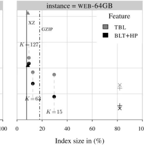
0 20 40 60 80 100 0 2 4 6 8 Index size in (%) Time per character in ( µs ) XZ GZIP K= 15 K= 63 K= 127 Index FM-HF-R3_K FM-RLMN FM-HF-V FM-HF-1L instance =WEB-64MB Index size in (%) 0 20 40 60 80 100 XZ GZIP K= 15 K= 63 K= 127 Feature TBL BLT+HP instance =WEB-64GB

Figure 10. Count time and space of our index implementations on input instances of different size with compression effectiveness baselines using standard compression utilitiesXZandGZIPwith option--best. FM-RLMN profits from each feature. Especially replacing the lookup table version forpopcnt

andselect64with more efficientBLTversions discussed above. Since FM-RLMN is a rather complex structure the differentrankandselectsub data structures “compete” for cache. As expected the

FM-index based onRANK-1L is slower than FM-HF-V when no optimization is used but slightly faster whenBLTandHPare activated. This reflects the outcome of the experiments of the basicrankdata structures used in both indexes shown in Figure 3.

Finally we discuss the time-space trade-offs of the different index types in Figure 10. As discussed above, optimizationsBLTand hugepages only affects the runtime performance on larger data sets (right). The uncompressed representations FM-HF-V and FM-HF-1L, and FM-RLMN are affected the most by the features. The FM-indexes based onH0compressed bitvectors are also affected. Interestingly, the indexes forK= 63and128achieve better compression then ourgzip --best baseline. The FM-index usingRANK-R3_K_and_K_{= 128}_{is only}_5%_{larger than the}_xz_compressed representation of the test input. The index forK= 256is even smaller but is not shown in Figure 10 due to the increased runtime as shown in Table IX.

Overall our new data structures, improvements and optimized implementations enable FM-indexes that are faster than the state of the art (usingRANK-1L) or smaller than state of the art indexes (usingRANK-R3_K_with_K_{= 128}_,_255).

7. CONCLUSION

We proposed a simple, cache-friendly rank data structure, a practical select data structure for uncompressed bitvectors and an improved implementation of compressed bitvector representations. We explore the behavior of rank and select data structures for binary and general sequences for varying data sizes, implementations, instruction sets and operating system features. We show that using the built-inpopcnt and our optimized select64 operation significantly improve the performance of classic rank and select data structures. We further discuss the effect of larger page sizes on the performance of succinct data structures. We demonstrate that these improvements propagate directly to more complex succinct data structures such as FM-indexes. Using larger page sizes has not yet been explored in literature in the context of succinct data structures and

Copyright c 0000 John Wiley & Sons, Ltd. Softw. Pract. Exper.(0000)

Prepared usingspeauth.cls DOI: 10.1002/spe

(46)

Experimental results: construction

Resource diagram for the construction of a Self-Index for 200MB of English text.

(47)

(48)

More WT operations: Query point grids

σ

n

Operations:

count(x₀,x₁,y₀,y₁) # points in rectangle[x0,x1][y0,y1].

(49)

CSA

ω2 0 ω1 0 ω3 0 ω3 0 # 1 ω1 0 ω1 0 ω4 0 ω1 0 # 1 ω1 0 ω4 0 ω3 0 ω1 0 # 1 ω5 0 ω5 0 # 1 T = b= 0 1 2 3 4 5 6 7 8 9 10 11 12 13 14 15 16 17 4 0 9 1 14 2 17 3 8 1 13 2 5 1 6 1 1 0 10 2 12 2 0 0 3 0 2 0 7 1 11 2 16 3 15 3 D= position=

ω

1

(50)

WT application: Top-

k

document retrieval

Represent document arrayDas wavelet tree

First explore nodes, which contain the maximal interval Example: Search top-2 documents (frequency based ranking)

012312110220001233 001101000110000111 0111100001 0111100001 00000 0 11111 1 0 23222233 01000011 22222 0 333 1 1

(51)

012312110220001233 001101000110000111 0111100001 0111100001 00000 0 11111 1 0 23222233 01000011 22222 0 333 1 1

(52)

WT application: Top-

k

document retrieval

012312110220001233 001101000110000111 0111100001 0111100001 00000 0 11111 1 0 23222233 01000011 22222 0 333 1 1

(53)

012312110220001233 001101000110000111 0111100001 0111100001 00000 0 11111 1 0 23222233 01000011 22222 0 333 1 1

(54)

WT application: Top-

k

document retrieval

012312110220001233 001101000110000111 0111100001 0111100001 00000 0 11111 1 0 23222233 01000011 22222 0 333 1 1

(55)

Other results:

2n+o(n)structure answers document frequency in constant time (Sadakane 2007)

Use RMQs for document listing (Sadakane 2007)

Prestore selected intervals (Hon et al. 2009). Use skeleton Suffix Tree for mapping.

(56)

Outline

(57)

Applications

Graphs (deBruijn subgraph, web graph,...) Lists (Inverted Lists,...)

monotone sequenceX with 0≤x₀≤x₁≤. . .≤x_m₋₁≤n.

Lower`=blog_mncbits stored explicitly.

Upper bits as sequenceH of unary encoded gaps Uses 2+blog_mncbits per element

(58)

Compressed Bitvectors: SD-array (Elias-Fano coding)

X = δ = H= L= 6 00110 1 2 01 2 1 1-0 8 01000 2 0 01 0 1 2-1 9 01001 2 1 1 1 0 2-2 17 10001 4 1 001 1 2 4-2 17 10001 4 1 1 1 0 4-4 31 11111 7 3 0001 3 3 7-4 X[3]=rank0(H,select1(H,4))·22+L[3] =4·4+1=17

(59)

InterpretX as positions of set bits in a bitvectorb. Constant timeacccess,rank,selectonb. Well suited for sparse bitvectors.

b= H= L= 0 0 0 1 0 2 0 3 0 4 0 5 1 6 0 7 1 8 1 9 0 0 0 1 0 2 0 3 0 4 0 5 0 6 1 7 0 8 0 9 0 0 0 1 0 2 0 3 0 4 0 5 0 6 0 7 0 8 0 9 0 0 0 1 01 2 01 0 1 1 001 1 1 1 0001 3

select(b,4) =rank0(H,select1(H,4))·22+L[3] =4·4+1=17

rank(b,i)andaccess(b,i): useselect0onH to select right upper part + scan left for entry inL

(60)

Balanced Parentheses Sequences (BPS)

Represent BPS as bitvector.

(()()(()())(()((()())()()))()((()())(()(()()))()))

find_open(i) Find matching closing paren ofBPS[i].

find_close(P) Find matching opening paren ofBPS[i].

enclose(i) Find tightest paren pair which encloses pair (i,find_close(i))

and more (double_enclose(i,j),rank(i),select(i),. . . ) can be answered in constant time by just addingo(n)space. (Munro 1996, Geary et al. 2004 & 2006)

(61)

Application: Succinct representation of trees 15 $ 7 dumulmum$ 11 m$ 3 ndumulmum$ lmu 14$ 9 m$ 1 ndumulmum$ lmu 12 m$ 4 ndumulmum$ u m 6 ndumulmum$ 10 m$ 2 ndumulmum$ lmu 13 $ 8 m$ 0 ndumulmum$ ulmu m 5 ndumulmum$ u (()()(()())(()((()())()()))()((()())(()(()()))())) BPSdfs= tree uncompressed O(nlogn)bits compressed 4nbits

(62)

Balanced Parentheses Sequences (BPS)

Application: Succinct representation of trees

15 $ 7 dumulmum$ 11 m$ 3 ndumulmum$ lmu 14$ 9 m$ 1 ndumulmum$ lmu 12 m$ 4 ndumulmum$ u m 6 ndumulmum$ 10 m$ 2 ndumulmum$ lmu 13 $ 8 m$ 0 ndumulmum$ ulmu m 5 ndumulmum$ u (()()(()())(()((()())()()))()((()())(()(()()))())) BPSdfs=( BPSdfs= 0 tree uncompressed O(nlogn)bits compressed 4nbits

(63)

Application: Succinct representation of trees 15 $ 7 dumulmum$ 11 m$ 3 ndumulmum$ lmu 14$ 9 m$ 1 ndumulmum$ lmu 12 m$ 4 ndumulmum$ u m 6 ndumulmum$ 10 m$ 2 ndumulmum$ lmu 13 $ 8 m$ 0 ndumulmum$ ulmu m 5 ndumulmum$ u (()()(()())(()((()())()()))()((()())(()(()()))())) BPSdfs=(( BPSdfs= 0 1 tree uncompressed O(nlogn)bits compressed 4nbits

(64)

Balanced Parentheses Sequences (BPS)

15 $ 7 dumulmum$ 11 m$ 3 ndumulmum$ lmu 14$ 9 m$ 1 ndumulmum$ lmu 12 m$ 4 ndumulmum$ u m 6 ndumulmum$ 10 m$ 2 ndumulmum$ lmu 13 $ 8 m$ 0 ndumulmum$ ulmu m 5 ndumulmum$ u (()()(()())(()((()())()()))()((()())(()(()()))())) BPSdfs=(() BPSdfs= 0 1 tree uncompressed O(nlogn)bits compressed 4nbits

(65)

Application: Succinct representation of trees 15 $ 7 dumulmum$ 11 m$ 3 ndumulmum$ lmu 14$ 9 m$ 1 ndumulmum$ lmu 12 m$ 4 ndumulmum$ u m 6 ndumulmum$ 10 m$ 2 ndumulmum$ lmu 13 $ 8 m$ 0 ndumulmum$ ulmu m 5 ndumulmum$ u (()()(()())(()((()())()()))()((()())(()(()()))())) BPSdfs=(()( BPSdfs= 0 1 3 tree uncompressed O(nlogn)bits compressed 4nbits

(66)

Balanced Parentheses Sequences (BPS)

15 $ 7 dumulmum$ 11 m$ 3 ndumulmum$ lmu 14$ 9 m$ 1 ndumulmum$ lmu 12 m$ 4 ndumulmum$ u m 6 ndumulmum$ 10 m$ 2 ndumulmum$ lmu 13 $ 8 m$ 0 ndumulmum$ ulmu m 5 ndumulmum$ u (()()(()())(()((()())()()))()((()())(()(()()))())) BPSdfs=(()() BPSdfs= 0 1 3 tree uncompressed O(nlogn)bits compressed 4nbits

(67)

Application: Succinct representation of trees 15 $ 7 dumulmum$ 11 m$ 3 ndumulmum$ lmu 14$ 9 m$ 1 ndumulmum$ lmu 12 m$ 4 ndumulmum$ u m 6 ndumulmum$ 10 m$ 2 ndumulmum$ lmu 13 $ 8 m$ 0 ndumulmum$ ulmu m 5 ndumulmum$ u (()()(()())(()((()())()()))()((()())(()(()()))())) BPSdfs=(()()( BPSdfs= 0 1 3 5 tree uncompressed O(nlogn)bits compressed 4nbits

(68)

Balanced Parentheses Sequences (BPS)

15 $ 7 dumulmum$ 11 m$ 3 ndumulmum$ lmu 14$ 9 m$ 1 ndumulmum$ lmu 12 m$ 4 ndumulmum$ u m 6 ndumulmum$ 10 m$ 2 ndumulmum$ lmu 13 $ 8 m$ 0 ndumulmum$ ulmu m 5 ndumulmum$ u (()()(()())(()((()())()()))()((()())(()(()()))())) BPSdfs=(()()(( BPSdfs= 0 1 3 5 6 tree uncompressed O(nlogn)bits compressed 4nbits

(69)

Application: Succinct representation of trees 15 $ 7 dumulmum$ 11 m$ 3 ndumulmum$ lmu 14$ 9 m$ 1 ndumulmum$ lmu 12 m$ 4 ndumulmum$ u m 6 ndumulmum$ 10 m$ 2 ndumulmum$ lmu 13 $ 8 m$ 0 ndumulmum$ ulmu m 5 ndumulmum$ u (()()(()())(()((()())()()))()((()())(()(()()))())) BPSdfs=(()()(() BPSdfs= 0 1 3 5 6 tree uncompressed O(nlogn)bits compressed 4nbits

(70)

Balanced Parentheses Sequences (BPS)

15 $ 7 dumulmum$ 11 m$ 3 ndumulmum$ lmu 14$ 9 m$ 1 ndumulmum$ lmu 12 m$ 4 ndumulmum$ u m 6 ndumulmum$ 10 m$ 2 ndumulmum$ lmu 13 $ 8 m$ 0 ndumulmum$ ulmu m 5 ndumulmum$ u (()()(()())(()((()())()()))()((()())(()(()()))())) BPSdfs=(()()(()( BPSdfs= 0 1 3 5 6 8 tree uncompressed_O (nlogn)bits compressed 4nbits

(71)

Application: Succinct representation of trees 15 $ 7 dumulmum$ 11 m$ 3 ndumulmum$ lmu 14$ 9 m$ 1 ndumulmum$ lmu 12 m$ 4 ndumulmum$ u m 6 ndumulmum$ 10 m$ 2 ndumulmum$ lmu 13 $ 8 m$ 0 ndumulmum$ ulmu m 5 ndumulmum$ u (()()(()())(()((()())()()))()((()())(()(()()))())) BPSdfs=(()()(()() BPSdfs= 0 1 3 5 6 8 tree uncompressed_O (nlogn)bits compressed 4nbits

(72)

Balanced Parentheses Sequences (BPS)

15 $ 7 dumulmum$ 11 m$ 3 ndumulmum$ lmu 14$ 9 m$ 1 ndumulmum$ lmu 12 m$ 4 ndumulmum$ u m 6 ndumulmum$ 10 m$ 2 ndumulmum$ lmu 13 $ 8 m$ 0 ndumulmum$ ulmu m 5 ndumulmum$ u (()()(()())(()((()())()()))()((()())(()(()()))())) BPSdfs=(()()(()()) BPSdfs= 0 1 3 5 6 8 0 1 3 5 6 8 11 12 ₁₄ 15 16 18 21 23 27 29 30 31 33 36 37 39 40 42 46 tree uncompressed O(nlogn)bits compressed 4nbits

(73)

Application: Range Minimum Queries

ArrayX ofnelements from a well-ordered set.

rmq(i,j)returns position of minimum element inX[i,j]. 2n+o(n)bits andO(1)time solution (Fischer & Heun 2011)

X =1 0 4 1 6 2 2 3 99 4 10 5 5 6 13 7 2 8 74 9 32 10 rmq(2,6)=3

(74)

Compressed Suffix Trees (CST)

15 $ 7 dum ulm um$ 11 m$ 3 ndum ulm um$ lm u 14 $ 9 m$ 1 ndum ulm um$ lm u 12 m$ 4 ndum ulm um$ u m 6 ndum ulm um$ 10 m$ 2 ndum ulm um$ lm u 13 $ 8 m$ 0 ndum ulm um$ ulm u m 5 ndum ulm um$ u 15 7 11 3 14 9 1 12 4 6 10 2 13 8 0 5 0 0 0 3 0 1 5 2 2 0 0 4 1 2 6 1 (()()(()())(()((()())()()))()((()())(()(()()))())) Full functionality... root() is leaf(v) parent(v) degree(v) child(v,c) select child(v,i) sibling(v) depth(v) lca(v,w) sl(v),wl(v,c) id(v),inv_id(i) Size: |CSA|+|LCP|+|BPS|, i.e. about original text size

(75)

Resource diagram for the construction of a CST for 200MB of English text.

(76)

Outline

(77)

https://github.com/simongog/sdsl-lite Input from about 40 research papers

Fast and space-efficient construction

Index structures available for byte and integer alphabets Well-optimized (e.g. hardware POPCOUNT, hugepages,... ) Easy configuration of myriads of CSAs, CSTs, WTs

Fast prototyping

(78)

Outline

(79)

Limitations/Challenges of Succinct Structures: Often only work for a static setting

Memory access pattern often non-local Implementation from scratch difficult Construction is often the bottleneck

Algorithms have to be adapted to work fast with succinct structures

(80)

Conclusion

Advantages of Succinct Structures:

Allow indexation of larger data sets (about 10-100 larger compared to classical indexes).

Adapt to the data: E.g. capture repetitions. Often provide more functionality.

More functionality often produces conceptional easier solutions.

(81)

Many applications heavily depend on Indexes. Self-Indexes made it possible to process Next Generation Sequencing inGenomics andLife Sciences.

Why?

Only the speed of self indexes matches the amazing throughput of sequencing technologies.

(82)

Succinct Data Structures: From Theory to Practice