OF MARGINAL UTILITY
Orazio P. Attanasio and Tullio Jappelli*
Abstract—The theory of intertemporal choice predicts that the cross-sectional variance of the marginal utility of consumption is equal to its own lag plus a constant and a random component. Using general prefer-ence specifications and some assumptions about the nature of the random component, we provide an explicit test of this hypothesis. Our approach circumvents the necessity to identify a pure age profile of the cross-sectional variance of consumption and yields a well-specified statistical test. This test is applied to data from the United States, the United Kingdom, and Italy. The results are remarkably consistent with the restrictions implied by the theory of intertemporal consumption choices.
I. Introduction
O
ne remarkable prediction of the permanent-income hypothesis with certainty equivalence is that consump-tion inequality within a group of households with fixed membership should, on average and over long periods of time, increase with age. By this model, the change in individual consumption represents the annuity value of the revisions in labor income, which (under rational expecta-tions) are unpredictable. Then, if income shocks are not perfectly correlated within the group, the cross-sectional variance of consumption increases with age until retirement (that is, until uncertainty is resolved). This prediction of the theory was first investigated by Deaton and Paxson (1994), who estimate the age profile of the cross-sectional variance of consumption using average cohort data for the United States, the United Kingdom, and Taiwan and find that consumption inequality increases with age in all three coun-tries.If certainty equivalence is relaxed, the permanent-income hypothesis provides predictions about the marginal utility of consumption, and not consumption itself. In particular, the model does not generate an explicit relation between age and consumption inequality or, for that matter, between consumption and income. We thus propose to focus directly on the Euler equation for consumption, and consider the time-series properties of the cross-sectional variance of an approximation of the marginal utility of consumption rather than consumption. Under the identifying assumptions dis-cussed in section II, the theory implies that, in a regression of the cross-sectional variance of the marginal utility of
consumption on a constant and its own lag, the coefficient of the latter is unity. We test this hypothesis in this paper. Our procedure does not require certainty equivalence; does not impose assumptions regarding the relation between age, time, and cohort effects in estimating the age profile of the cross-sectional variance; and delivers a simple statistical test of a well-specified null hypothesis that allows us to apply standard inference tools.
The benefits are not cost free, however. The test we propose is based on assumptions regarding the properties of the residuals of the Euler equation. A rejection of the null hypothesis could therefore be due to the failure of these assumptions and not necessarily of the permanent income model. Furthermore, because we relax certainty equiva-lence, we cannot exploit the relation between consumption, income innovations, and age. For instance, we cannot check if the increase in consumption inequality slows around retirement, as implied by the certainty equivalence case. Nor can we attribute the spreading of consumption inequal-ity to permanent and transitory changes in uncertainty, as Blundell and Preston (1998) propose.
We use average cohort data to test our hypothesis. In the absence of long panel data on consumption, these data are particularly well suited to the problem at hand. Although we cannot compute the cross-sectional variance of the same group of individuals over time, average cohort data allow us to track the variance of a representative sample of the same cohort. Another advantage of cohort data is that they allow us to apply an appropriate instrumental variables estimator. The empirical analysis, presented in section III, uses three approximations to the marginal utility of consumption. Ini-tially, we measure marginal utility as the log of expenditure on nondurable goods. We then take into account the life-cycle variations of family size and define marginal utility as the log of nondurable consumption expenditure per adult equivalent. Finally, we compute marginal utility by relying on available estimates of the parameters of a flexible utility function. These parameters have been estimated with the same data sets used in this paper. Having estimated the marginal utility for each household in the sample, we can then compute the cross-sectional variance of marginal util-ity of population groups defined by year of birth and test whether the coefficient of lagged variance on current vari-ance is unity. The advantage of the third procedure is that marginal utility is allowed to depend upon a full set of demographic and labor supply variables.
We use three sets of cohort data. The British Family Expenditure Survey (1974–1993) and the U.S. Consumer Expenditure Survey (1980–1995) cover a sufficiently long timespan and allow consistent estimation of an Euler
equa-Received for publication May 28, 1998. Revision accepted for publica-tion May 23, 2000.
* University College London, Institute for Fiscal Studies, CEPR, and NBER; and CSEF, University of Salerno, and CEPR, respectively.
We would like to thank James Banks, Richard Blundell, Luigi Pistaferri, and Guglielmo Weber for useful comments and suggestions, and Sarah Tanner for help with the U.K. data. Particular thanks are owed to Angus Deaton and Christina Paxson for interesting discussions and extensive exchanges that we hope improved the paper. We retain responsibility for any errors. This paper is part of the research project, “Structural Analysis of Household Savings and Wealth Positions over the Life-Cycle.” The Training and Mobility of Researchers Network Program (TMR) of the European Commission DGXII and the Italian National Research Council (CNR) provided financial support.
The Review of Economics and Statistics,February 2001, 83(1): 13–27
tion for consumption. We also use data drawn from the Italian Survey of Household Income and Wealth (1987– 1995); because this is too short a timespan to provide reliable estimates of the Euler equation, in this case we do not attempt to measure marginal utility by using a flexible utility function. Section IV summarizes the results.
II. The Cross-Sectional Variance of Marginal Utility
We take off from Deaton and Paxson (1994) and their exploration of the implications of the permanent-income hypothesis for the evolution of consumption and income inequality. It is well known that, if the utility function is quadratic and if the real interest rate equals the discount rate, optimal consumption for individual i follows a mar-tingale:
ci,t⫹1⫽ci,t⫹⑀i,t⫹1 (1)
The cross-sectional variance of the variables in equation (1) is
var共ci,t⫹1兲⫽var共ci,t兲⫹var共⑀i,t⫹1兲⫹cov共ci,t,⑀i,t⫹1兲, (2)
in which variances and covariances are computed over a cross section of households whose composition is constant over time. If aggregate variables are part of the information set of each agent, Deaton and Paxson (1994) show that the time average of cov (ci,t, ⑀i,t⫹1) is zero. Equation (2) then implies that, in a group with fixed membership, the variance of consumption of individuals agedtis stochastically dom-inated by the variance of consumption of the same individ-uals agedt ⫹1. In other terms, in a stationary population, consumption inequality increases with age on average and over long periods of time. Because ⑀i,t⫹1 represents the annuity value of the innovations in permanent income, consumption inequality increases until individuals face in-come shocks. Such dispersion should at least slow down for older households if earnings shocks dominate interest-rate shocks.
A. Relaxing Certainty Equivalence
Equation (1) and (2) can be generalized to more-flexible preference specifications. Suppose that utility is intertem-porally separable and that the instantaneous utility function, defined over nondurable consumption, depends on a set of conditioning variablesz (demographic and labor supply, let us say), and on an unobservable component,v, that captures unobserved heterogeneity. In this case, it can be immedi-ately shown that the Euler equation that applies to individ-uali is
Et关共ci,t⫹1,⬘zi,t⫹1, vi,t⫹1兲共1⫹rtk⫹1兲兴
(3)
⫽共ci,t,⬘zi,t,vi,t兲
whereis the marginal utility of consumption,
rtk⫹1 is the rate of return on a generic assetk,
is a set of parameters of the utility function, and
 ⫽ 1/(1⫹ ␦) is the discount factor.
Note that bothandare assumed to be time invariant and common to all individuals.
Inspection of equation (3) reveals that, if one abandons the assumption of quadratic utility in favor of more-general preference specifications, it becomes very difficult to derive a relationship between the cross-sectional variance of the level of consumption and age. Before investigating in detail the implications of the general specification in equation (3) and discussing our approach, it is useful to consider some simple examples in which the lifecycle model does not necessarily imply that the cross-sectional variance of con-sumption increases with age. Deaton and Paxson (1994) also discuss some of these situations.
A simple situation in which, even with quadratic utility, the cross-sectional variance of utility does not necessarily increases over time is when the discount factor differs from the rate of interest. The Euler equation is then ci,t⫹1 ⫽ constant ⫹ (1 ⫹ ␦)/(1 ⫹ r)ci,t ⫹ ⑀i,t. If r ⬎ ␦, then consumption increases on average over the lifecycle, rein-forcing the effect of the variance of the innovation term. If insteadr ⬍ ␦, consumption declines over the lifecycle. In the absence of income shocks, the cross-sectional variance of consumption would then also fall with age. Income innovations may partly or completely offset the tendency of the variance to fall with age. Note that, with uncertain lifetimes, the risk of longevity makes consumers effectively more impatient, raising the possibility of a declining con-sumption path, particularly in old age.
Another simple example in which the variance of con-sumption does not necessarily increase is one with no uncertainty and isoelastic utility, so that the Euler equation is ln ci,t⫹1⫽ lnci,t⫹ (r ⫺ ␦), where is the intertem-poral rate of substitution. Clearly, although var (lnci,t⫹1) is constant for each age group, var (ci,t⫹1) increases with age ifr ⬎ ␦ and declines if r ⬍ ␦.
The situation in which there is no uncertainty is equiva-lent, as far as the cross-sectional variance of consumption is concerned, to a situation in which individual shocks are perfectly insured. As with perfect insurance, the only shocks to consumption are aggregate ones, and the cross-sectional variance of the marginal utility of consumption is constant over time. Whether the level of cross-sectional variance of consumption increases depends on the nature of preferences and on the relative size of interest rate and discount factor. For instance, with isoelastic preferences and the interest rate less than the discount factor, the cross-sectional variance of consumption levels declines with age.1
1These first two examples indicate that, if one were interested in
As discussed by Deaton and Paxson (1994), another case in which the lifecycle pattern of the cross-sectional variance of consumption is not obvious is one in which demographic (or other variables) affect the marginal utility of consump-tion. If, for instance, utility is defined in terms of per capita, rather than total consumption, with quadratic preferences, the Euler equation takes the formci,t⫹1/Ni,t⫹1⫽ ci,t/Ni,t ⫹
⑀i,t. The lifecycle pattern of the cross-sectional variance of consumption depends now not only on the cross-sectional variance of the shocks but also on the cross-sectional variability (and its changes over time) in family size.2 A similar argument can be made with respect to any age-related preference shift (thez variables in equation (3)).
The final example is one with isoelastic utility and non-insurable shocks. If the distribution of consumption growth is log normal, one obtains an exact Euler equation with a term for precautionary saving:
lnci,t⫹1⫽ln ci,t⫹共r⫺␦兲⫹共⫺1/ 2兲
⫻ 关var共⌬ln ci,t⫹1兲兴⫹⑀t⫹1,
where⫺1is the coefficient of relative prudence and⑀ t⫹1an expectational error.3Computing the cross-sectional variance of both sides of the Euler equation, one sees that the spreading of consumption depends also on the age evolution of the conditional variance of consumption growth. We know very little about this term and how it varies across consumers as they age, which thus makes the predictions of the model hard to pin down.
The examples show that, with slight departures from the simplest model with certainty equivalence, consumption inequality can increase or decrease with age, depending on demographics, preferences, and the gap between the dis-count and interest rates. It should also be clear that the age pattern of consumption levels is not the same as that of consumption logs. The same applies to the marginal utility of consumption. Looking again at equation (3) one sees that the cross-sectional variance of marginal utility declines with age for precisely the same reasons for which one expects the variance of consumption to increase with age.
Even though the relationships between age and the vari-ances of consumption levels, log consumption, and mar-ginal utility are ambiguous, the theory does have predictions about the dynamics of consumption inequality. Our ap-proach consists, therefore, in focusing on the time-series
autocorrelation of the cross-sectional variance of the mar-ginal utility of consumption. As an example, consider again equation (2). One can see that a regression of the cross-sectional variance of consumption—proportional to the marginal utility of consumption under quadratic utility—on its lagged value should yield, under some conditions, a coefficient of unity.
To see how this point extends to more-general situations such as equation (3), we consider the case wherein the instantaneous utility function is isoelastic, that is:
U共c,z, v兲⫽ ci,t
1⫺⫺1
1⫺⫺1exp关⫺⫺ 1共⬘z
i,t⫺vi,t兲兴.
The Euler equation (3) can now be expressed as a linear function of the logarithm of consumption:
ln共ci,t⫹1兲⫹⬘zi,t⫹1⫺vi,t⫹1
(4)
⫽ln  ⫹ln 共ci,t兲⫹⬘zi,t⫺vi,t⫹˜i,t⫹1
⫹ ln 共1⫹rt⫹1
k 兲⫹⑀ ˜i,t⫹1
⫽ln  ⫹ln 共ci,t兲⫹⬘zi,t⫺vi,t⫹i
⫹ ln 共1⫹rtk⫹1兲⫹⑀ i,t⫹1,
whereis the elasticity of intertemporal substitution,
⑀
˜i,t⫹1 is an expectational error, and
˜i,t⫹1 is the higher conditional moments of the distribu-tion of consumpdistribu-tion in equadistribu-tion (3).4
The second equality in equation (4) follows by defining
⑀i,t⫹1 ⫽ ˜i,t⫹1 ⫺ i ⫹ ⑀˜i,t⫹1, where i indicates the time-series average of the conditional moments. The cross-sectional variance of the two sides of equation (4) is
varln共ci,t⫹1兲⫹⬘zi,t⫹1⫹vi,t⫹1
(5)
⫽var关ln 共ci,t兲⫹⬘zi,t⫹vi,t兴⫹var共i兲
⫹var共⑀i,t⫹1兲⫹2cov关ln 共ci,t兲,i⫹⑀i,t⫹1兴.
Equation (5), as such, cannot be measured empirically. (For one thing, the parametersare unknown. Second, the variablevis by definition unobservable. Finally,includes unknown parameters and moments of a distribution that has not yet been specified.) But equation (5) does highlight a sharp prediction of the theory: that the coefficient of the lagged cross-sectional variance of marginal utility equals 1.5 It is precisely because of this property that, in the simple
former is a better approximation of marginal utility when preferences are isoelastic. Furthermore, because consideration of the log of consumption implicitly implies the consideration of a log linearization, the result is independent of the relative size of interest rate and discount factor. Deaton and Paxson focus mainly on the pattern of the variance of log consump-tion.
2The cross-sectional variance of the number of adult equivalents (used
in the later empirical exercises) is flat in the very first part of the lifecycle, increases in middle age, and decreases in the last part of the lifecycle. The same is true for the variance of the logs of adult equivalents.
3The variance in this Euler equation is the time-series variance of
consumption growth for each consumer.
4For instance, if the interest rate is constant and consumption growth is
normally distributed, this term equals the conditional variance of con-sumption growth.
5The left side of equation (4) is not exactly the marginal utility of
case of quadratic utility, the cross-sectional variance of consumption increases, on average, with age. In the remain-ing portion of this section, we illustrate how we propose to test this important implication of intertemporal optimiza-tion.
To make equation (5) operational, we need to make a number of identifying assumptions. We deal with the first problem (that the parameter vector is unknown) below. For the present, we assume thatis known. To address the fact thatvandare unobservable, one can write equation (4) as
ln共ci,t⫹1兲⫹⬘zi,t⫹1
(6)
⫽ln  ⫹ln共ci,t兲⫹⬘zi,t⫹i
⫹ ln共1⫹rtk⫹1兲⫹⌬
vi,t⫹1⫹⑀i,t⫹1.
Assuming that the real interest rate is common across households, the cross-sectional variance of the two sides of equation (6) is given by the following expression:
varln共ci,t⫹1兲⫹⬘zi,t⫹1
(7)
⫽varln共ci,t兲⫹⬘zi,t
⫹var 共i⫹⌬vi,t⫹1⫹⑀i,t⫹1兲
⫹2 cov关ln共ci,t兲⫹⬘zi,t,i⫺⌬vi,t⫹1⫹⑀i,t⫹1兴.
Only the first term on the right side can be measured empirically using cross-sectional data. However, the second and third terms can be decomposed into a part that is constant over time (such as the variance of and its covariance with the other components) and a time-variant component. Equation (7) can then be rewritten as
var关ln 共ci,t⫹1兲⫹⬘zi,t⫹1兴
(8)
⫽0⫹E共t⫹1兲⫹var关ln 共ci,t兲⫹⬘zi,t兴
⫹t⫹1⫺E共t⫹1兲
⫽0⫹var关ln 共ci,t兲⫹⬘zi,t兴⫹t⫹1,
whereE(t⫹1) denotes the time series average oft⫹1;
0 includes the time-invariant terms of the right side of equation (7):
0⫽var共i兲⫹2 cov关ln 共ci,t兲⫹ ⬘zi,t, i兴
⫹ 2 cov关i,⌬vi,t⫹1兴⫹ 2 cov共i, ⑀i,t⫹1兲; and
t⫹1 denotes the time-varying components of the cross-sectional variance:
t⫹1⫽var共⌬vi,t⫹1兲⫹var共⑀i,t⫹1兲⫹2 cov 关ln共ci,t兲
⫹ ⬘zi,t,⌬vi,t⫹1]⫹2 cov共⌬vi,t⫹1,⑀i,t⫹1兲.
The terms0andt⫹1are implicitly defined by the second equality in equation (8). Note that most components oft⫹1 do not vanish. An exception is cov (i, ⑀i,t⫹1), which is 0 under the permanent income hypothesis.
B. The Empirical Test
Suppose now that we can identify one or more population groups whose membership is fixed over time. The cross-sectional variances in equation (8) can then be estimated by computing the corresponding sample variances within groups at different time periods. This application of syn-thetic panel techniques yields consistent estimates of the corresponding population variances. We can then run the regression
var关ln 共ci,t⫹1兲⫹⬘zi,t⫹1兴
(9)
⫽0⫹var关ln 共ci,t兲⫹⬘zi,t兴⫹t⫹1
and test the hypothesis that ⫽1.
The use of OLS to estimate equation (9) would produce inconsistent estimates of , however, for at least three reasons. First, the hypothesis that the cross-sectional covari-ance of ⌬vi,t⫹1 with the observed component of marginal utility at timetis 0 is likely to be violated. Second, the time varying-terms included in t⫹1 might be correlated over time with the variance term in equation (8). Finally, in a finite sample, one never observes the true population mo-ments, but only an estimate of these moments that are therefore affected by measurement error. This induces a further source of bias in the estimate of.
Thus, the issue is that of finding an instrument for var [ln (ci,t) ⫹ ⬘zi,t] that is uncorrelated with t⫹1 and with the sampling error. Synthetic cohort data suggest an ideal candidate for dealing with the potential bias arising from measurement error: if the samples used in estimating the variances in equation (9) are independent—as they typically are in repeated cross sections—so are the sample errors of subsequent periods. Therefore, var [ln (ci,t⫺1) ⫹
⬘zi,t⫺1] is, as far as sampling error is concerned, a valid instrument for the corresponding variance at time t with which it is obviously correlated. However, to guarantee that the (twice) lagged variance is a valid instrument overall, one must assume that cov {t⫹1, var [ln (ci,t⫺1)⫹⬘zi,t⫺1]}⫽ 0, that is, that the twice-lagged variance is uncorrelated with the deviation oft⫹1from its unconditional mean. This is a strong assumption that deserves further scrutiny.
To better understand the issues involved, it is worthwhile to strip the model down to its simplest version, the one with certainty equivalence behind equation (1) and (2), wherein
from its time mean, however, is not an implication of the permanent-income hypothesis. Rather, its validity depends on the nature of the shocks⑀i,t⫹1, on the agents’ information set as well as on the market structure in which they operate. Suppose that the expectational error of the Euler equation is described by ⑀i,t⫹1 ⫽ ␣it⫹1 ⫹ i,t⫹1 where t⫹1 is an aggregate shock and i,t⫹1 is an idiosyncratic shock as-sumed to be i.i.d. across individuals and over time and independent of ␣i and t⫹1. (Notice that the aggregate shock is allowed to affect consumers in different fashion.) This representation of the error term encompasses several models.6
Given the assumed structure of the error term, var (⑀i,t⫹1) ⫽ t2⫹1var (␣i) ⫹ var (i,t⫹1). If i,t⫹1 is indeed i.i.d., then var (i,t⫹1) is constant over time. Iftis also i.i.d.—so that E(t2⫹1) is constant over time— cov [var (⑀i,t⫹1), var (ci,t)] ⫽ 0, and var (ci,t⫺1) is obvi-ously a valid instrument for var (ci,t). If instead t is heteroskedastic and/ort2⫹1exhibits a considerable amount of persistence, then var (ci,t⫺1) may not be a valid instru-ment for var (ci,t). For instance, if the conditional time variance of t⫹1 follows an ARCH(1) process, cov [var (⑀i,t⫹1), var (ci,t)] ⫽ 0, and our instrument is still a valid one; but, ift2⫹1 evolves according to an ARCH of order 2 or higher (or as any GARCH process), it is not. Similar arguments apply toi,t⫹1 and to its cross-sectional variance.
Although we develop the previous example with qua-dratic utility, the same considerations apply to the more general model that relaxes certainty equivalence. In partic-ular, when the innovations to the Euler equation can be decomposed into an aggregate shock and an individual-specific shock, the period t ⫺ 1 variance of the marginal utility of consumption is a valid instrument for its periodt variance if
● the aggregate shock is part of the agents’ information set,
● its second moments do not exhibit persistence over time, and
● the evolution of the cross-sectional variance of the idiosyncratic shocks is not correlated with the cross-sectional variance of consumption.
These are not predictions of the permanent-income/lifecycle model. Thus, our test that ⫽1 is a joint test of the model and these additional assumptions. A finding that ⫽ 1 cannot therefore be taken necessarily as a contradiction of the model, but a finding that ⫽1 implies that the model and our additional assumptions are consistent with the data. We also experiment with an alternative instrument for var [ln (ci,t) ⫹ ⬘zi,t]. Theory suggests that, in the case of
certainty equivalence, the cross-sectional variance of con-sumption is an increasing function of age, so that age is likely to be correlated with the dependent variable even relaxing certainty equivalence. However, for age to be a valid instrument, one must assume that it is uncorrelated with the cross-sectional variance ofi,t and with the time variance oft. The latter assumption is quite plausible. The former, however, is questionable, especially when one con-siders periods of the lifecycle during which uncertainty changes in a dramatic and yet systematic way. The most obvious example is retirement. For this reason, in the empirical section we use age both in addition to and in place of the lagged variance as an instrument for the current variance. We also check if our estimates ofare sensitive to the inclusion of the retired in our samples.
Notice that the hypothesis that ⫽ 1 holds both under the lifecycle model with uninsurable shocks and under perfect insurance. In this sense, our approach (unlike Deaton and Paxson’s (1994)) cannot be used to discriminate between these two models. However, not all models imply such a relationship. To see why this is the case, consider a model in which some consumers might be liquidity con-strained. For a generic consumer i at time t, the Euler equation for consumption is
共ci,t, zi,t,vi,t兲
⫽Et关共ci,t,zi,t,vi,t兲共1⫹r兲/共1⫹␦兲兴⫹i,t
wherei,tis the Kuhn-Tucker multiplier associated with the liquidity constraint for consumeriat timet. Therefore, this term equals 0 for those consumers that are not liquidity constrained. If one thinks that such multipliers are related, when positive, to the level of income, one sees that the cross-sectional variance of consumption is related not only to its lagged value, but also to the value of the cross-sectional variance of income.7 Furthermore, as the number of liquidity-constrained consumers is likely to vary over the business cycle, one would not expect the coefficient of the lagged variance of consumption to be unity.
C. Measuring Marginal Utility and Its Cross-Sectional Variance
The problem that the parameter vectoris unknown can be handled in several ways. The simplest strategy is to drop thez variables and regress the variance of log consumption on the lagged variance. A more satisfactory measure of marginal utility is to assume thatzincludes only family size and to scale the consumption data using adult equivalent weights. This is equivalent to assuming that the utility
6In the case of complete contingent markets, for instance, the error term
has the factor structure⑀i,t⫹1⫽t⫹1⫹i,t⫹1, wherei,t⫹1 is i.i.d and
independent oft⫹1.
7Another model that does not predict ⫽1 is the myopic model of
consumption,ci,t⫽yi,t. One sees immediately that ⫽0 here and that
function is defined on consumption per adult equivalent, rather than on consumption,
U共c,P,N兲⫽ Ni,t 1⫺⫺1
冉
ci,t Pi,t
冊
1⫺⫺1
and estimate
var
冋
ln冉
ci,t⫹1 Pi,t⫹1冊
⫹ln
冉
Pi,t⫹1Ni,t⫹1
冊册
(10)
⫽0⫹var
冋
ln冉
ci,t Pi,t
冊
⫹ln
冉
Pi,tNi,t
冊册
⫹i⫹1
where Pi,t is the number of adult equivalents, Ni,t is the number of household’s members, andis the elasticity of intertemporal substitution.8
A third possibility is to posit more-flexible preference specifications that explicitly allow the utility function to depend on labor supply and demographic variables. Be-cause the preference parameters are unknown, they have to be estimated from the data. We propose the following approach. In a first stage, we use the same cohort data and exploit the orthogonality conditions implied by the Euler equation to estimate the parameters of the utility function. In a second stage, we use the estimated parameters to compute the cross-sectional variance in equation (9) and to test the hypothesis that ⫽1. In section III, rather than performing the first stage, we rely on previous estimates. In particular, we use preference parameters estimated by Euler equations that have been fitted to the same data sets used in this paper.9 In all cases, we estimate equation (9) and (10) for all cohorts simultaneously. Because the population groups (cohorts) might be characterized by different variances inandv, we always check if the results are sensitive to the introduction of dummies for cohort-specific intercepts.
As discussed in subsection IIB, in the presence of (occa-sionally) binding liquidity constraints, the cross-sectional variance of (log) consumption would not only depend on its lagged value but also on the cross-sectional variance of the Kuhn-Tucker multiplier associated with the constraints. As such multipliers are likely to be related to current income, we test for the presence of the variance of lagged income into our regression equations.
D. Comparison with Deaton and Paxson’s Methodology
Average cohort data lend themselves very well to the problem at hand. By definition, birth cohorts are groups with fixed membership.10The most intuitive way of testing the implications of equation (5) is to track the cross-sectional variance of the marginal utility as the cohort ages. Indeed, in their seminal contribution, Deaton and Paxson (1994) constructed average cohort data for the United States, the United Kingdom, and Taiwan, considering the graphical representation of the cross-sectional variance and testing the hypothesis that the variance of (log) consumption increases with age.
Their methodology therefore involves identifying an age profile of the cross-sectional variance. This amounts to disentangling age, time, and cohort effects. Because these variables are perfectly collinear (time ⫽ cohort ⫹ age), Deaton and Paxson normalize the time effects to 0, so that the evolution over time of the cross-sectional variances of each cohort is explained only by a combination of age and cohort effects.11 Without structural and/or out-of-sample information, this normalization is indispensable: Any time trend can be written as a combination of age and cohort effects, and any age effect can be written as a combination of year and cohort effects.
The normalization is essentially an issue of interpretation when describing average cohort profiles of consumption or wages. In the case at hand, however, the implication of the theory being tested is of a structural relationship between age and the cross-sectional variance, and the assumption that all variance trends are explained by cohort and age effects is not particularly appealing. This problem is partic-ularly relevant for the sample period that Deaton and Pax-son consider, at least for the United States and the United Kingdom. During the 1980s, there was a considerable in-crease in inequality that affected all cohorts and was partly related to the increase in the return to education. Our approach completely circumvents this identification issue by focusing on the implication that the coefficient on the lagged variance (that is, the coefficientin equation (9)) is equal to unity. A related advantage is that it tests a well-defined null hypothesis against which standard inference tools can be applied.
8The second term in the square brackets in equation (10) appears if
utility is defined in terms of consumption per adult equivalent but is then summed over the number of family members rather than adult equivalents. With log utility, the expression simplifies to one in which consumption per capita enters the marginal utility. In practice, the inclusion of the second term does not make much difference for the results we obtain.
9A more efficient strategy, which we do not pursue here, might be to
consider equation (6) and (9) as a simultaneous equations system. This would be equivalent to estimating the parameters of the utility function exploiting the restrictions that the theory implies on the time series of both first and second cross-sectional moments. One could then use the over-identifying restrictions (including ⫽1) to test the model. This procedure would also have the advantage of explicitly taking into account the fact that the vectoris unknown.
10To be more precise, Deaton and Paxson (1994) assume that time
effects have zero mean and are orthogonal to a linear trend. This allows identification of all coefficients of interest. They also assume that age, time, and cohort effect do not interact. We are abstracting here from differential mortality and immigration. Because our samples are not restricted to couples, we also abstract from differential divorce rates.
11A slightly less restrictive assumption would be that the average of the
Another important difference between our approach and Deaton and Paxson’s is that focusing on the autocorrelation properties of the cross-sectional variance of the marginal utility avoids the problems that are caused by the fact that, in many plausible situations (some of which we discussed in subsection IIA), the cross-sectional variance of consump-tion does not increase with time. Our approach lends itself naturally to the consideration of preference specifications that are more flexible than quadratic, such as those that allow for a precautionary saving motive. Furthermore, we do not need to assume any relationship between the interest rate and the discount factor and/or the constancy over time of the former.
Our approach, however, is not without disadvantages. First of all, we can obtain consistent estimates of the coefficient in equation (9) only under a number of assump-tions that were discussed at length in subsecassump-tions IIA and IIB. Furthermore, unlike Deaton and Paxson’s approach, ours does not identify the lifecycle profile of consumption inequality and therefore cannot be used to discriminate between a model with perfect insurance and a standard lifecycle model with uninsurable individual shocks. Be-cause of this, we can say that our approach is a complement to—rather than a substitute for—Deaton and Paxson’s.
III. Empirical Results
We present our empirical evidence in three parts. We first describe the data sets used, then provide a graphical illus-tration of the main feature of the cross-sectional variance of consumption and marginal utility, and finally report the results of our econometric analysis. Some of the details of the data treatment are given in appendix A.
A. Data Description
We estimate equation (9) and (10) using three sets of average cohort data. The U.K. Family Expenditure Survey is the largest dataset, including twenty annual surveys (1974–1993). The U.S. Current Expenditure Survey is avail-able for sixteen years (1980–1995). The Italian Survey of Household Income and Wealth is available from 1984 to 1995, but, given the characteristics of this survey, we use data from only 1987 to 1995. Furthermore, the Italian data is available every other year, so that we can use a total of five surveys. Our choice to focus on the United States, the United Kingdom, and Italy was guided mainly by the availability of cohort data for these countries.
The FES: The main motivation for the collection of the Family Expenditure Survey (FES) on the part of the U.K. Department of Employment is the computation of the weights for the retail price index. In recent years, the data set has been used extensively to describe the behavior of U.K. households and to estimate structural models of con-sumption behavior. The sample includes approximately
7,000 households per year. (The survey has no panel ele-ment.) Each household stays in the sample for two weeks, during which it compiles a diary with its expenditures. At the end the diary is collected, and further information on various expenditure items during the previous three months (typically durable goods and utilities) is gathered. The survey also takes information on several economic and demographic household characteristics, ranging from labor supply to household composition. The quality of the con-sumption data (thanks especially to the use of the diary method rather than retrospective interviews) is remarkably good.12
As each household stays in the sample for just two weeks, consumption figures are heavily affected by seasonality. This problem is particularly serious for the cross-sectional variances we compute. For instance, part of the difference in consumption between a respondent interviewed in Decem-ber and one interviewed in August certainly is due to seasonal effects and not to genuine cross-sectional variabil-ity. To account for this, we deseasonalize the individual consumption observations before computing the cross-sec-tional variance. The seasonal adjustment is described in appendix A.
The CEX: The Consumer Expenditure Survey (CEX) is run by the U.S. Bureau of Labor Statistics for the same reasons as the FES (namely to compute the consumer price index), and the size of the sample is roughly similar (ap-proximately 7,000 households per year). Like the FES, the CEX also collects data on income, demographics, and several other variables.13There are, however, two important differences between the two. First, the CEX has a short panel element, in that each household is interviewed five times over fifteen months. The first interview is only a contact interview on which no information is disclosed in the public-use tape; in each of the subsequent four inter-views, however, the household reports detailed information on the expenditures incurred during each of the three pre-vious months. Potentially, that is, each household provides twelve monthly expenditure accounts. Second, the house-holds in the CEX do not compile a diary but answer retrospective questions.
The households in the CEX do not complete their cycle of interviews simultaneously. Because interviews are per-formed every month, households interviewed in different months report information on different periods. For
exam-12A recent study edited by Banks and Johnson (1997) compares
expen-diture and income data in the FES with those of the national accounts. It finds that—controlling for differences in definitions (especially of housing services), reference population, and sampling structure—the FES data track very well their counterparts in the national accounts.
13Some questions are asked only in the last or in the first and last
ple, a household that completes its last interview in January 1990 provides information on each of the twelve months of 1989, and a household that completes its cycle of interviews in June 1990 covers the period from June 1989 to May 1990. One-twelfth of the sample is replaced each month, and of course not all households complete the cycle of five interviews.
This sampling structure complicates the computations of the cross-sectional variances in which we are interested. We cannot compute the cross-sectional variance in a given year using the monthly observations as we do in the FES because several observations would refer to a single household. Variation across monthly observations would therefore re-flect time-series (seasonal or cyclical) rather than cross-sectional variability. Estimating annual consumption for each household is complicated by the overlapping structure of the sample: the “year” over which we have information for each household would be different depending on the month in which the household completes its cycle of inter-views. Annual estimates are further complicated by the fact that not all households complete the cycle.
We consider two possible methods of constructing the cross-sectional variances. The first is to estimate the “cal-endar year” consumption figure for each household on the basis of the months available, with seasonal adjustment. By this method, most households would provide figures to be used in the computation of the variance in two different years, and this should be taken into account in the choice of instruments. The second procedure involves considering only one monthly observation per household; after seasonal adjustment one can compute the cross-sectional variance for all the households in a given quarter or year.
We use the second procedure. Its drawback, however, is that, by limiting itself to one observation per household, it wastes useful information. On the other hand, it is simple to apply and yields a sample whose structure is very similar to that of the FES. To minimize the effect of nonrandom attrition, the monthly observation we select is the first available. The procedure for seasonal adjustment is the same one used for the FES (detailed in appendix A).
The SHIW: The primary purpose of the Bank of Italy Survey of Household Income and Wealth (SHIW) is to collect detailed data on demographics and households’ in-come and wealth. It uses a representative sample of the Italian resident population, and probability selection is en-forced at every stage of sampling. Like the FES and the CEX, it samples the household, defined as all persons residing in the same dwelling and related by blood, mar-riage, or adoption. The SHIW consumption data are col-lected by retrospective questions on broad categories of durable and nondurable consumption during the previous year. This implies that seasonal adjustment is not necessary. Given the different purpose of the survey, the detail and quality of the consumption data is not as high as that in the
FES or the CEX. Nonetheless, the SHIW consumption data match the trends in the national accounts data reasonably well. The sample size is slightly larger than that of the other two surveys (approximately 8,000 households).
Until 1984, the age of the household head is available only in wide bands precluding the construction of year-of-birth cohorts. In 1986, the data for expenditures on durable goods is indistinguishable from nondurable consumption. Since 1987, the survey was conducted every other year. For our purpose, therefore, the only usable surveys are the five surveys taken from 1987 to 1995.
B. Measures of Marginal Utility
In all three surveys, we define consumption as total household expenditure on nondurable goods. This excludes expenditures on durable goods, health, education, and hous-ing—except in the case of the SHIW, where it excludes durable expenditure only. Our focus on nondurable con-sumption implies, implicitly, an ascon-sumption of separability with respect to the excluded components. Current values are transformed into constant values using a consumer price index. As discussed in section II, we use three different approximations of the marginal utility of consumption. The first is simply the logarithm of consumption, and the second is the log of consumption per adult equivalent. The third filters the consumption data using the preference parameters estimated by Attanasio and Weber (1993) for the United Kingdom and by Attanasio and Weber (1995) for the United States. The definition of adult equivalent used in the second procedure assigns a weight of 1 to the first adult, 0.8 to any additional adult, and 0.25 to any child. To compute the expressions in equation (10), it is also necessary to know the value of the elasticity of intertemporal substitution. Those reported in the following tables correspond to a value of of 0.8. We experimented with alternative specifications, both for the definition of adult equivalent and for the assumption about the elasticity of intertemporal substitu-tion, and we obtained very similar results.14
The SHIW allows a straightforward estimation of the variance of annual log consumption. The sample size and structure of the FES and CEX allow us to construct quar-terly data. The results for the United Kingdom and the United States using annual observations are similar to those presented in the following subsections and can thus be omitted for brevity. The only notable difference is that the standard errors for the United States based on annual ob-servations are slightly larger than those based on quarterly observations.
C. Cohort Definition and Descriptive Analysis
In each survey, we restrict the sample to households that are headed by individuals born between 1910 and 1959 and
define ten groups: cohort 1 includes those born in 1910– 1914, cohort 2 those born in 1915–1919, and so on, up to cohort 10 from 1955–1959. We define the age of the cohort as the median age of each cohort in a given sample period. (For instance, the age of cohort 1, born in 1910–1914, is 68 in 1980, 69 in 1981, and so on.)
Table 1 reports the cohort definition and, for each survey, the mean and minimum cell size by cohort. The assumption behind our procedure is that the cross-sectional variance refers to the same group of individuals at different points in time. Even though we do not need to observe the same individuals over time, the test requires that the sample composition be constant. The positive correlation between survival probabilities and wealth implies that rich house-holds are overrepresented in the older cohorts. The
correla-tion between wealth and young headship (young working adults living independently are likely to be wealthier than average) suggests that rich households may also be over-represented in the youngest cohorts. Accordingly, we ex-clude households in which the head is older than eighty or younger than twenty.
The construction of cohort data involves taking means of the marginal utility within each of the cells over successive time periods. Aggregation, however, is not an issue in this context. Each of the methods of measuring the marginal utility of consumption first defines an index of marginal utility at the household level; the cross-sectional variance of this index can then be readily computed within each cell.
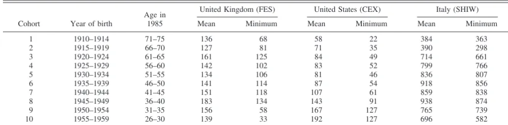
Before presenting the regression results, we provide a graphical exposition of the data. In figure 1, we plot the
TABLE1.—AVERAGE ANDMINIMUMCELLSIZE IN THEFES,THECEX,AND THESHIW
Cohort Year of birth
Age in 1985
United Kingdom (FES) United States (CEX) Italy (SHIW)
Mean Minimum Mean Minimum Mean Minimum
1 1910–1914 71–75 136 68 58 22 384 363
2 1915–1919 66–70 127 81 71 35 390 298
3 1920–1924 61–65 161 125 84 49 714 661
4 1925–1929 56–60 142 102 83 52 799 766
5 1930–1934 51–55 134 106 81 46 836 807
6 1935–1939 46–50 141 114 87 54 918 856
7 1940–1944 41–45 151 118 107 61 859 838
8 1945–1949 36–40 183 134 143 91 938 874
9 1950–1954 31–35 156 58 167 127 765 739
10 1955–1959 26–30 139 33 192 127 696 582
The table reports the average and minimum cell size in the Family Expenditure Survey (FES), the Consumer Expenditure Survey (CEX), and the Survey of Household Income and Wealth (SHIW) by year of birth. The cells are used to compute the variance of log consumption.
TABLE2.—REGRESSIONS FOR THEVARIANCE OFLOGCONSUMPTION
Country var (lnci,t) var (lnyi,t) p-value Instrument set
First-stage R-squared
Number of observations
United Kingdom 0.945 0.14 var (lnci,t⫺1) 0.52 766
(0.037)
0.996 0.91 age, age2 0.48 776
(0.039)
0.969 0.38 age, age2, 0.59 766
(0.035) var (lnci,t⫺1)
1.019 ⫺0.059 0.72 age, age2, 0.61 766
(0.056) (0.058) var (lnci,t⫺1), 0.24
var (lnyi,t⫺1)
United States 0.724 0.04 var (lnci,t⫺1) 0.10 620
(0.134)
1.012 0.90 age, age2 0.24 630
(0.096)
0.972 0.77 age, age2, 0.25 620
(0.094) var (lnci,t⫺1)
0.969 ⫺0.021 0.75 age, age2, 0.25 620
(0.09) (0.037) var (lnci,t⫺1), 0.22
var (lnyi,t⫺1)
Italy 0.798 0.11 var (lnci,t⫺1) 0.63 28
(0.123)
0.830 0.12 age, age2 0.71 38
(0.106)
0.773 0.05 age, age2, 0.79 28
(0.108) var (lnci,t⫺1)
0.924 ⫺0.254 0.58 age, age2, 0.80 28
(0.134) (0.143) var (lnci,t⫺1), 0.30
var (lnyi,t⫺1)
cross-sectional variance of the logarithm of consumption for the United Kingdom, the United States, and Italy, respec-tively. Each connected segment refers to a different cohort, observed over time at different ages. The cohort numbers, let us recall, run from 1 (the oldest) to 10 (the youngest). To facilitate the comparison across countries, the graphs are plotted on the same scale. These graphs are similar to the raw variances produced by Deaton and Paxson (1994). (See their figures 2 and 3 for the United States and the United Kingdom, respectively.)15
As we stress in section II, interpreting these graphs is not easy because cohort, age, and time are perfectly collinear variables. Their distinct effects are not identified: for in-stance, any interpretation of the data in terms of age and cohort effects (normalizing time effects to 0) can be recast in terms of an alternative decomposition in terms of age and time effects (normalizing cohort effects to 0). Nonetheless, some features of the raw data are highly suggestive.
Interestingly, the absolute level of the variance is consid-erably higher in the United States (0.4 on average), lowest in Italy (0.25), and intermediate in the United Kingdom (0.3), reflecting very different patterns of consumption in-equality in these countries. In the United Kingdom, there is some evidence of cohort effects, especially for households born after the second world war (cohorts 7 to 10 in figure 1). In the United States and Italy, cohort effects are absent or
weak at best. In the United Kingdom and Italy, the variance of log consumption increases up to age sixty and diminishes for older households, which Deaton and Paxson interpret as evidence in support of models with finite horizon, in which income shocks cease after retirement. The graph for the United States, by contrast, is much flatter over the entire lifecycle.16
In figure 2, we plot the cross-sectional variance of log consumption defined in terms of adult equivalent, assuming an intertemporal elasticity of substitution of 0.8. (See equa-tion (10).) The behavior of these variances is rather different than in the previous figures in all three countries. First of all, the variance is now considerably smaller, especially in the United Kingdom. Second, the age pattern is much flatter than in the previous set of figures, suggesting that variation in household size and composition over the lifecycle ex-plains a good part of the age profile of the cross-sectional variance of consumption. In the United Kingdom and the United States, there is no evidence of the spreading of consumption over the lifecycle. In Italy, the cross-sectional variance declines slightly with the age of the household head, reversing the pattern in figure 1.17
15As mentioned, in the estimation for the United Kingdom and the
United States, we use the variance of quarterly (log) consumption. To have legible pictures, we plot the variance only for the first quarter of each year and for five cohorts (2, 4, 6, 8, and 10).
16The pattern of inequality may reflect also differences in measurement
of consumption in the different surveys.
17Using a flexible specification of preferences to impute marginal utility
further reduces the cross-sectional variance in the United Kingdom and the United States. There is again weak evidence of age effects in con-sumption inequality only in the United Kingdom. For brevity, these figures are not reported.
FIGURE 1.—THE VARIANCE OF LOG CONSUMPTION
The last set of figures summarizes the age effect in the cross-sectional variance according to the different measures of marginal utility that are available in each of the three countries. The age effect is obtained by regressing the cross-sectional variance against a fifth-order age polynomial, a full set of cohort dummies, and a set of time dummies constrained to sum to 0 and to be orthogonal to a time trend.18 The estimated age pro-files show that consumption inequality increases with age only for the variance of log consumption. Even in this case, however, the age effects show little spread-ing of consumption. Figure 3 shows that in the United Kingdom, the variance increases only from 0.2 to 0.4, in the United States from 0.35 to 0.5, and in Italy from 0.15 to 0.30. If instead consumption is defined in terms of adult equivalent or if we directly impute marginal utility, we find flat (or even declining) age profiles of the cross-sectional variance in each of the three coun-tries.
The pattern of the estimated age effects contrasts slightly with the findings of Deaton and Paxson, particularly in the case of the United States. Using the CEX, they find that the age effects in the United States increase from approximately 0.2 to 0.5 (while ours grows from 0.35 to 0.5) for both the variance of the logarithm of consumption and the variance computed defining consumption per adult equivalent. Part of the difference may derive from differences in the
treat-ment of the data or different sample periods.19They also use quarterly cells, but limit the analysis to the 1980–1990 period. However, computing the age effects after dropping the 1991–1995 years does not change the profiles in fig-ure 3.
As we discussed in section II, only under special assump-tions does the theory deliver a closed-form solution for consumption and allow a test of the hypothesis that con-sumption inequality increases with age on average and over long periods of time. Furthermore, such a prediction of the theory is testable only by arbitrarily normalizing the time effects. Using Deaton and Paxson’s methodology, this pre-diction of the theory is rejected in each of the three data sets when we take into account the fact that part of the inequality in consumption over the lifecycle is explained by variation in household size and composition. We now turn to our alternative—and, in some respects, more general—test of the implication of intertemporal choices for the evolution of the cross-sectional variance of the marginal utility of con-sumption.
D. Regression Results
We regress the variance of log consumption on its own lag (see equation (9)) for the three countries for which we have data. Table 2 reports the point estimates, the standard
18This procedure differs slightly from that used by Deaton and Paxson
because we use a polynomial in age rather than age dummies. This, however, does not affect our results in any substantive way.
19Before computing the cross-sectional variance, we adjust our
con-sumption figures using a model that allows monthly seasonal effects. Furthermore, to avoid complicated MA structures due to the overlapping structure of the sample as well as biases induced by nonrandom attrition, we use only the first interview completed by each household.
FIGURE 2.—THE VARIANCE OF LOG CONSUMPTION PERADULT EQUIVALENT
errors, thep-value of a test that the coefficient of the lagged variance equals 1, and theR-square of the first-stage regres-sion. The basic specification for the variance of marginal utility also included a full set of cohort dummies. However, an F-test for the significance of the cohort dummies was never statistically different from 0, regardless of the mea-sure of marginal utility. The cohort dummies are therefore dropped in the final specifications.
As is shown in section II, OLS estimates of equation (9) are potentially subject to measurement error and endogene-ity bias. Thus, for each specification, we report four sets of results. The first three regressions differ in instruments used. The first uses only the second lag of the cross-sectional variance; the second replaces the lagged variance with the (median) age and age square of the cohort; and the third includes age, age square, and the second lag of the variance. Finally, in the fourth line for each country and definition of marginal utility, we augment the regression with the lagged variance of household disposable income (instrumented with its second lag). Along with the estimate and standard error of the coefficient on the lagged variance of consump-tion (and income, when relevant), we report thep-value of a test of the hypothesis that ⫽1 and theR-square of the first-stage regression.
None of the regressions reported in table 2 rejects the null hypothesis that the coefficient of the lagged variance equals 1, with the exception of the third regression for Italy, where the test rejects the null hypothesis at the five-percent level. The coefficients of the lagged variance are generally
esti-mated with small standard errors, particularly in the case of the United Kingdom. Furthermore, the point estimates for the United States and the United Kingdom are remarkably close to 1 and similar across different sets of instruments. Note also that, in each regression, the instruments have explanatory power for var (lncit).
Our results are not affected by excluding the youngest and oldest cohorts or cohorts whose cells are not very large. For instance, excluding retired households (older than 57 years) does not affect the estimate of, regardless of the instruments that are used in the estimation.
As discussed in section II, the lagged cross-sectional variance of income might be relevant if earnings are related to the Kuhn-Tucker multipliers associated to liquidity con-straints. The fourth row for each country in table 2 shows that there is no evidence that this term plays a role in the regression for the cross-sectional variance of consumption. In table 3, the dependent variable is the cross-sectional variance of log consumption per adult equivalent, as in equation (10).20The estimates are not as precise as those in table 2, particularly for the United States, but the general pattern is confirmed. The magnitude of the estimated coef-ficients for the United Kingdom and the United States is hardly affected, although in Italy the point estimates are
20When the utility function is defined in terms of adult equivalent,
marginal utility depends on the elasticity of intertemporal substitution. The results in the tables refer to the case in which the parameter equals 0.8. Different values yield similar results.
FIGURE 3.—ESTIMATED AGE EFFECTS
much closer to 1. In no case can the hypothesis that ⫽1 be rejected at conventional significance levels. The only exception is the first regression for the United States. Note, however, that in this case the correlation between var (lncit) and var (lncit⫺1) is very low, resulting in a value for R-squared in the first-stage regression of only 0.01. The results reported in table 3 are again robust to the exclusion from the sample of the oldest cohorts and to the inclusion of the lagged income variance as an additional regressor.
In table 4, we compute marginal utility using the speci-fication
U共c,z兲⫽ ci,t
1⫺⫺1
1⫺⫺1exp共⫺⬘zi,t兲,
in whichz includes family size and indicator variables for blue-collar workers, heads out of employment, full-time working spouse, and more than two income recipients. This specification of the instantaneous utility function has been estimated by Attanasio and Weber (1993, 1995) on the same FES and CEX cohort data. Thus, we can readily use their estimates of to compute marginal utility.21 The actual values of the estimates and the details about the construction
of marginal utility are described in appendix A. We do not attempt to fit a flexible Euler equation to Italian data. Due to the few surveys and the fact that we work with annual data, the number of observations is much lower than it is in the other two countries. The point estimate offor the United Kingdom and the United States in Table 4 are again very close to unity, regardless of the instrument set. Given also the small standard errors of the estimate, in no case can we reject the hypothesis that ⫽ 1. The point estimates obtained by dropping the retired do not show again appre-ciable differences as well as those including the lagged income variance.
Our results show that an important implication of the lifecycle model—namely that the coefficient on the lagged variance in equation (9) is equal to unity—is not rejected by the data. It may seem surprising that this result holds for all different measures of marginal utility. However, one should consider that our instrumental-variable strategy and the fact that we are working with isoelastic specifications would give us consistent estimates of the parameter of interest as long as the instruments used are uncorrelated with the omitted variables (for instance, with the cross-sectional variance of adult equivalents).
21If the intertemporal elasticity of substitution, , is constant across
households, it represents only a factor of proportionality that does not affect the regression results. Attanasio and Weber (1993) also consider seasonal shifts of preferences. Because these shifts are assumed to be
multiplicative and constant across consumers, they do not affect the computation of the cross-sectional variance.
TABLE3.—REGRESSIONS FOR THEVARIANCE OFLOGCONSUMPTIONPERADULTEQUIVALENT
Country var (lnci,t) var (lnyi,t) p-value Instrument set
First-stage R-squared
Number of observations
United Kingdom 0.912 0.24 var (lnci,t⫺1) 0.22 766
(0.075)
1.029 0.80 age, age2 0.11 776
(0.112)
0.942 0.41 age, age2, 0.26 766
(0.070) var (lnci,t⫺1)
0.959 ⫺0.002 0.78 age, age2, 0.28 766
(0.152) (0.088) var (lnci,t⫺1), 0.19
var (lnyi,t⫺1)
United States ⫺0.039 0.01 var (lnci,t⫺1) 0.01 620
(0.403)
0.944 0.82 age, age2 0.05 630
(0.245)
0.839 0.48 age, age2, 0.05 620
(0.227) var (lnci,t⫺1)
0.847 ⫺0.011 0.50 age, age2, 0.05 620
(0.23) (0.033) var (lnci,t⫺1), 0.22
var (lnyi,t⫺1)
Italy 1.121 0.74 var (lnci,t⫺1) 0.21 28
(0.362)
0.930 0.71 age, age2 0.62 38
(0.190)
0.987 0.94 age, age2, 0.68 28
(0.185) var (lnci,t⫺1)
0.968 ⫺0.041 0.94 age, age2, 0.68 28
(0.451) (0.210) var (lnci,t⫺1), 0.69
var (lnyi,t⫺1)
The table reports coefficient estimates of the regression
varln共ci,t⫹1/Pi,t⫹1兲⫹ln共Pi,t⫹1/Ni,t⫹1兲⫽0⫹varln共ci,t/Pi,t兲⫹ln共Pi,t/Ni,t兲⫹t⫹1.
IV. Conclusions
The lifecycle hypothesis predicts that the cross-sectional variance of the marginal utility of consumption is equal to its own lag plus a constant and a random component. Using fairly general preference specifications and auxiliary as-sumptions about the nature of the random component, we provide an explicit test of this hypothesis. Our approach circumvents the necessity to identify a pure age profile of the cross-sectional variance of consumption and yields a well-specified statistical test. On the other hand, the test we propose is valid only under specific assumptions about the shocks of the Euler equation for consumption.
Cohort data for the United Kingdom, the United States, and Italy provide strong support for the hypothesis that the coefficient of the lagged cross-sectional variance of mar-ginal utility is equal to 1. That is, the joint hypothesis that the theoretical restrictions on the evolution of the cross-sectional variance and the auxiliary identification assump-tions we use are consistent with the data.
As we have repeatedly stressed, our test does not assume certainty equivalence. Rather, we are able to confront with the data a flexible representation of preferences that allows for departures from certainty equivalence, dependence on family size, labor supply, and other demographic variables. This increased generality, however, has a price: we loose the ability to relate the evolution of the cross-sectional variance of consumption to the evolution of the cross-sectional vari-ance of earnings. This relation has proven to be particularly useful in welfare comparisons among households.
Blundell and Preston (1998) study under which condi-tions consumption is a better indicator of welfare inequality than income. They note that, in the lifecycle model, cross-sectional comparisons of consumption inequality are infor-mative about welfare inequality only on restrictive assump-tions that concern the form of the utility function. They also
show that under certainty equivalence the evolution of the variance of consumption should reflect permanent-income innovations, whereas the variance of earnings should reflect permanent as well as transitory changes in uncertainty. Our study is complementary to theirs in that it shows that one of the most general implications of individuals’ intertemporal choices for the evolution of the cross-sectional variance is borne out by the data.
Dropping certainty equivalence, only simulation analysis can give an idea of the structural relation between the cross-sectional variances of earnings and consumption (ex-amples of such simulation models are in Hubbard, Skinner, and Zeldes (1995)). In principle, these models could simu-late the consumption behavior of a generation and compute the evolution of the cross-sectional variance of marginal utility. By changing the stochastic properties of the income-generating process, it would then be possible to study the relation between income and consumption inequality. We regard this as an interesting topic for future research.
REFERENCES
Attanasio, Orazio P., and Guglielmo Weber, “Consumption Growth, the Interest Rate and Aggregation,”Review of Economic Studies60 (July 1993), 631–649.
“Is Consumption Growth Consistent With Intertemporal Optimi-zation? Evidence from the Consumer Expenditure Survey,” Jour-nal of Political Economy103 (December 1995), 1121–1157. Banks, James, and Paul Johnson,How Reliable Is The Family Expenditure
Survey Data. Trends in Incomes and Expenditure over Time. (London: Institute for Fiscal Studies, 1997).
Blundell, Richard, and Ian Preston, “Consumption Inequality and Income Uncertainty,” Quarterly Journal of Economics113 (May 1998), 603–640.
Deaton, Angus, and Christina Paxson, “Intertemporal Choice and Inequal-ity,”Journal of Political Economy102 (June 1994), 437–467. Hubbard, Glenn R., Jonathan Skinner, and Stephen P. Zeldes,
“Precau-tionary Saving and Social Insurance,”Journal of Political Econ-omy103 (April 1995), 360–399.
TABLE4.—REGRESSIONS FOR THEVARIANCECOMPUTED WITHFLEXIBLEPREFERENCESPECIFICATION
Country var (lnci,t) var (lnyi,t) p-value Instrument set
First-stage R-squared
Number of observations
United Kingdom 0.924 0.26 var [u⬘(ci,t⫺1)] 0.26 766
(0.068)
1.001 0.93 age, age2 0.24 776
(0.073)
0.966 0.57 age, age2, 0.34 766
(0.066) var [u⬘(ci,t)]
0.996 ⫺0.034 0.95 age, age2, 0.36 766
(0.068) (0.046) var [u⬘(ci,t⫺1)], 0.22
var (lnyi,t⫺1)
United States 0.803 0.53 var [u⬘(ci,t⫺1)] 0.02 620
(0.310)
0.995 0.98 age, age2 0.07 630
(0.192)
0.947 0.77 age, age2, 0.08 620
(0.181) var [u⬘(ci,t)]
0.802 0.038 0.45 age, age2, 0.08 620
(0.261) (0.055) var [u⬘(ci,t⫺1)], 0.23
var (lnyi,t⫺1)