Carbon Dioxide Emission Prediction of Four CIS Countries by Applying a Correlation and GMDH Artificial Neural Network

Carbon Dioxide Emission Prediction of Four CIS Countries

by Applying a Correlation and GMDH Artificial Neural

Network

Mohammad Hossein Ahmadi1, Mahdi Ramezanizadeh2, Mohammad Alhuyi Nazari2,3,

Simin Kheradmand4, Shahab Shamshirband5,6

1_{Faculty of Mechanical of engineering, Shahrood University of Technology, Shahrood, Iran} 2_{Aerospace Engineering Department, Shahid Sattari Aeronautical University of Science and}

Technology, Tehran, Iran

3_{Faculty of New Sciences and Technologies, Tehran University, Tehran, Iran.} 4_{Faculty of Civil Engineering, Kharazmi University, Tehran, Iran.}

5_{Department for Management of Science and Technology Development, Ton Duc Thang}

University, Ho Chi Minh City, Vietnam

6 _{Faculty of Information Technology, Ton Duc Thang University, Ho Chi Minh City, Vietnam}

Corresponding author: [email protected]

Abstract

Increase in the emission of Greenhouse Gases (GHS) is among the significant concerns of government, societies, and policy-makers. Due to the highest share of carbon dioxide in the produced GHGs, it is necessary to assess the factors that influence its emission. Energy systems and economic activities noticeably influence the amount of carbon dioxide production of countries. In this article, Artificial Neural Network (ANN) in addition to a linear correlation used to predict carbon dioxide emission of four CIS countries, including Turkmenistan, Uzbekistan, Kazakhstan, and Azerbaijan based the consumption of various energy sources and GDP, as the economic indicator. According to the obtained data by the proposed models, carbon dioxide emission can be estimated by utilizing the mentioned input data. Models’ R-squared value are 0.9997 and 0.9999 in the cases of applying the correlation and ANN-based model. Moreover, the average absolute relative deviations by utilizing the correlation and GMDH ANN are approximately 1.05% and 0.61%, respectively. These statistical values demonstrate more proper performance of the ANN-based model compared with the applied linear correlation.

Keywords: Artificial Neural Network; Carbon dioxide; Greenhouse gases; GMDH; GDP

1. Introduction

Studies have shown that the economic activities influences on energy consumption. Also, the

emission of greenhouse gases (GHGs) depends on the energy system and its features [1]. Increase

in energy consumption causes a higher production of GHGs due to the noticeable share of fossil

fuels in the current energy systems [2]. World energy consumption and carbon dioxide emission

have significantly increased in recent decades, as illustrated in Figure 1. As it is represented, the

world’s total primary energy consumption increased from about 6627.1 Mtoe in 1980 to more than

13511 Mtoe in 2017. In a similar period, the carbon dioxide emission had increment form

approximately 18364 Mt to more than 33440 Mt. Moreover, it can be observed that the trend of

carbon dioxide emission and energy consumption is very similar to each other, which indicates

their dependency. In addition to energy utilization, level of economic activities has an impact on

GHGs emission.

Figure 1 Total primary energy consumption and carbon dioxide emission of the world [3] 15000 17000 19000 21000 23000 25000 27000 29000 31000 33000 35000 6000.0 7000.0 8000.0 9000.0 10000.0 11000.0 12000.0 13000.0 14000.0

1970 1980 1990 2000 2010 2020

C arb o n d io xi d e e m is si o n (M t) To ta l P ri m ary e n erg y co n su m p ti o n (M to e ) Year Energy Consumption

The increasing rate of energy consumption is mainly attributed to development in industrial and

economic activities, increment in population, and improved quality of life. Various ways are

suggested to overcome the energy-related GHG emission, such as improving the efficiency of the

technologies, using renewable energy sources, energy recovery, and energy audit [4–6]. Due to the

lower GHG emission of renewable energies in comparison with fossil fuels such as oil and coal

[7,8], there are several worldwide renewable energy projects [9–11]. Wind and solar energy

projects are among the most attractive and fast-growing types of renewable energy technologies

applicable to power generation, cooling, and heating [12,13]. In order to model the energy system

of a country, it is necessary to consider the share of various sources in the overall energy

consumption; therefore, both renewable sources and different kinds of fossil fuels must be

considered.

Various mathematical approaches are applicable to model the systems and forecast their behavior

[14–16]. Among the several methods used for system modeling, artificial neural networks (ANNs)

have proved their high-level precision due to their intelligent procedure and structure [17,18].

ANNs are used for recognition of patterns and estimating the output of a system based on defined

inputs [18–20]. The accuracy of the ANN-based model is highly dependent on the selection of

input data. According to a study conducted by Rezaei et al. [1] employed consumptions of energy

sources and GDP as input data is appropriate to accurately estimate carbon dioxide of some Nordic

countries [21]. In their study, the maximum value of absolute error was lower than 4%, showing

acceptable precision of the introduced model.

Since the prediction of carbon dioxide emission gets an appropriate insight into the potential ways

of its reduction, it is crucial to obtain a comprehensive and precise model. In this article, GMDH

four Commonwealth of Independent States (CIS) countries based on GDP, coal, oil, natural gas

and renewable energies consumption as the inputs of the model. The data used for modeling are

extracted from various references between 2000 and 2017 in order to have a comprehensive and

reliable dataset as the inputs of the models. Details on the employed algorithm and modeling

procedure explained in the following sections.

2. Method

A model is established by GMDH neural networks with the utilization of a multi-layer network

structure for a complex system based on the interactions of input-output data [22,23]. This neural

network is closely similar to feedforward neural networks. GMDH is a self-taught method

introduced by A.G. Ivakhnenko [24], and then, it is widely used for modeling of complex systems.

Each element in a neural network is literally a nonlinear equation between two inputs and one

output, and its coefficients are determined by regression methods. Useless elements are

automatically removed through the network construction process as a result of the inability to

specify the accurate output and beneficial connections of each hidden layer remain since they are

contributed in the precise prediction of the output and increase the total network efficiency. By

repeating these steps, the GMDH neural network is finally reached, with the lowest error and high

predictive power in determining the correct and close outcomes.

GMDH algorithm creates a model which is a collection of neurons in various layers. In other

words, this neural network is a self-organized network, consisting of several layers and several

neurons in each of the layers.

The network describes the approximate function of 𝑓̂ with the output of 𝑦̂ by combining quadratic

error in comparison to the actual output of y. Therefore, for the M experimentally measured data

comprised of n inputs and a single output, the actual results are stated as follows:

𝑦_𝑗 = 𝑓(𝑥_𝑗1, 𝑥_𝑗2, … , 𝑥_𝑗𝑀) (𝑗 = 1,2, … , 𝑀) (1)

The target is to achieve a neural network that can forecast the output value of 𝑦̂ for any input vector

of X. Hence:

𝑦̂𝑗 = 𝑓̂(𝑥𝑗1, 𝑥𝑗2, … , 𝑥𝑗𝑀) (𝑗 = 1,2, … , 𝑀) (2)

The proposed GMDH neural network should be able to minimize the squared error between the

actual and forecasted values, in other words:

∑(𝑦̂_𝑗2− 𝑦_𝑗2) → 𝑚𝑖𝑛

𝑀

𝑗=1

(3)

The relationship between input and output variables can be stated by using the polynomial function

as follows, i.e. Ivakhnenko polynomials:

𝑦 = 𝑎0+ ∑ 𝑎𝑖𝑥𝑖 𝑛

𝑖=1

+ ∑ ∑ 𝑎𝑖𝑗𝑥𝑖𝑥𝑗 𝑛

𝑗=1 𝑛

𝑖=1

(4)

In many cases, the quadratic and bivariate form of this polynomial is used as follows:

𝑦̂ = 𝐺(𝑥_𝑖, 𝑥_𝑗) = 𝑎₀+ 𝑎₁𝑥_𝑖 + 𝑎₂𝑥_𝑗+ 𝑎₃𝑥_𝑖2+ 𝑎₄𝑥_𝑗2+ 𝑎₅𝑥_𝑖𝑥_𝑗 (5)

The unknown coefficients of 𝑎_𝑖in Eq. (5) are determined by the regression method so that the

difference between the actual output of y and the calculated values of 𝑦̂ for each pair of input

variables, 𝑥_𝑖 and 𝑥_𝑗, is minimized. A set of polynomials is established by using Eq. (5). The

each function of Gi (each constructed neuron), the coefficients are obtained to minimize the total

neuron error in order to achieve optimal fit of the inputs with the total pair of output-input sets:

𝐸 =∑ (𝑦𝑖− 𝐺𝑖)

2 𝑀

𝑖

𝑀 → 𝑚𝑖𝑛

(6)

In the basic methods of the GMDH algorithm, all binary compounds (neurons) are constructed by

n input variables, and the unknown coefficients of the neurons are obtained using the least squares

approach. Therefore, (𝑛₂) =𝑛(𝑛−1)

2 neurons in the second layer are constructed as follows:

{(𝑦_𝑗, 𝑦𝑗𝑝, 𝑦𝑗𝑞)|(𝑗 = 1, 2, … , 𝑀)& 𝑝, 𝑞 ∈ (1,2, … , 𝑀} (7)

The second-order form of the expressed function, Eq. (6), is utilized for each M triple row. These

equations expressed in the following matrix form:

𝐴𝑎 = 𝑌 (8)

Where A represents the vector of unknown coefficients of the second order equation:

𝑎 = {𝑎₀, 𝑎₁, 𝑎₂, 𝑎₃, 𝑎₄, 𝑎₅} (9)

𝑌 = {𝑦1, 𝑦2, 𝑦3, … , 𝑦𝑀}𝑇 (10)

2 2

1 1 1 1 1 1

2 2

2 2 2 2 2 2

2 2

1

1

1

p q p q p q

p q p q p q

Mp Mq Mp Mq Mp Mq

A

x

x

x

x

x x

x

x

x

x

x x

x

x

x

x

x x

 

 

 

 

=

 

 

 

 

M M M M M M

(11)

By using the least squares method with the utilization of regression analysis:

𝑎 = (𝐴𝑇𝐴)−1𝐴𝑇𝐴 (12)

This equation gives the vector of coefficients of Eq. (6) for all M triple sets.

3. Results and discussion

In this paper, four CIS countries, including Uzbekistan, Turkmenistan, Azerbaijan and

Kazakhstan, are considered as the cases of the study. CIS countries have experienced economic

growth after 2000 as illustrated in Figure 2; as a consequence, due to the requirement of energy

for economic and industrial activities, their overall energy consumption has increased after 2000

as shown in Figure 3. According to Figure 3, the overall primary energy consumption of these

countries has increased from 104.57 Mtoe in 2000 to approximately 156 Mtoe in 2017 which

indicates average annual growth rate of 2.25%. Due to the dependency of environmental issues on

the economic activities of the countries and their energy consumption, it is crucial to analyze their

Figure 2 GDP of the investigated countries [3]

Figure 3 Total primary energy consumption of the investigated countries [3]

In addition to GDP, consumption of various conventional fuels must be used as input variables

due to the dependency of production of carbon dioxide on the type of fuels. The emission of carbon

dioxide from the combustion depends on their type as shown in Figure 4. Therefore, the input

variables of the model used for carbon dioxide estimation of carbon dioxide production are GDP,

0 50 100 150 200 250

2000 2005 2010 2015 2020

G D P (b ill io n U SD ) Year Azerbaijan Kazakhstan Turkmenistan Uzbekistan 0 10 20 30 40 50 60 70 80 90

2000 2005 2010 2015 2020

consumptions of oil, renewable energy sources (including hydropower and other renewable energy

consumptions), natural gas and coal which are similar to the previous study [1]. All the data utilized

for modeling are extracted in the period of 2000 and 2017.

Figure 4 Carbon dioxide emission of various fuels [25]

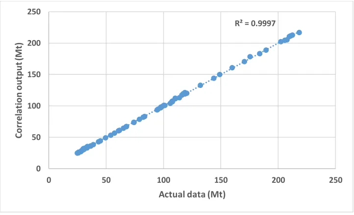
In the first step, a linear correlation is used to find the correlation between the inputs and output.

The obtained correlation by considering the mentioned data is:

Carbon Dioxide emission =−0.00283 ∗ 𝑥₁+ 2.860766 ∗ 𝑥₂+ 4.051923 ∗ 𝑥₃+ 2.382961 ∗

𝑥₄− 1.67667 ∗ 𝑥₅− 0.32311

Where 𝑥₁, 𝑥₂, 𝑥₃, 𝑥₄, and 𝑥₅ denote GDP, oil, coal, natural gas, and renewable energies

consumptions. Based on the calculated coefficients of the correlation, coal has the most significant

effect on the emission of 𝐶𝑂₂. In addition, since the coefficient of renewable energy is negative, it

can be concluded that development in the renewable energy systems leads to reduced GHG

emission. The actual outputs and the corresponded correlation values are represented in Figure 5.

As it is represented, the R-squared value by using the correlation is equal to 0.9997.

0 50 100 150 200 250 300 350 400 450

Hard coal Oil Natural gas

C ra b o n d io xi d e e m is si o n p er u n it o f e n e rr gy (k g/M Wh )

Figure 5 Actual data vs model's outputs in the case of applying linear correlation

In Figure 6, the relative deviation for each data index is represented. According to the comparison

between the correlation output and actual data, the highest absolute relative deviation is

approximately 5.01%. This value demonstrates acceptable accuracy of the correlation as a

predictive tool. The average absolute relative deviation of the proposed correlation is about 1.05%.

R² = 0.9997

0 50 100 150 200 250

0 50 100 150 200 250

C

o

rr

el

at

io

n

o

u

tp

u

t (M

t)

Figure 6 Relative deviation of model's outputs in the case of applying linear correlation

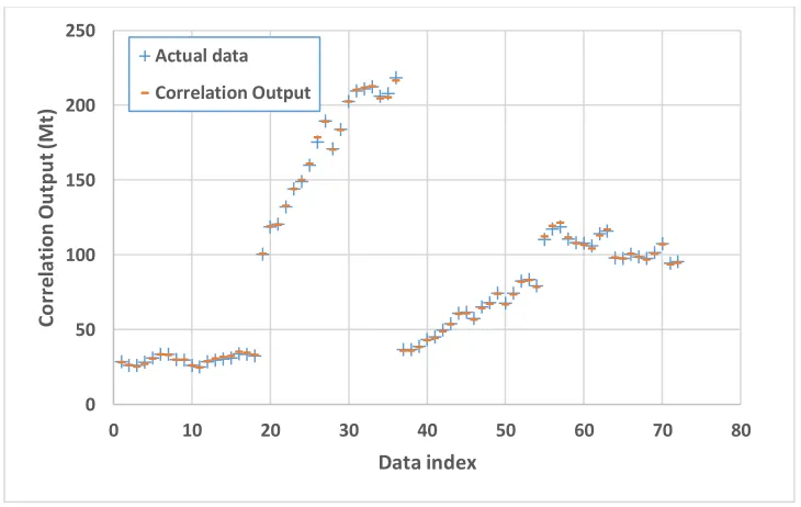
In Figure 7, the actual data and the corresponded calculated value by the correlation are represented.

Comparing the values, both actual ones and correlation outputs, reveals the precision of the

correlation in estimating 𝐶𝑂₂ emission of the investigated countries.

Figure 7 Figure 10 Comparison between model outputs and actual data in the case of applying linear correlation

-6 -5 -4 -3 -2 -1 0 1 2 3 4

0 10 20 30 40 50 60 70 80

R el at iv e d ev ia ti o n (% ) Data index 0 50 100 150 200 250

0 10 20 30 40 50 60 70 80

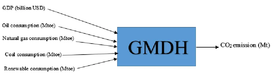
In addition to correlation, an ANN-based model is proposed to compare the results. The schematic

of the model is shown in Figure 8.

Figure 8 Schematic of the model

As it was indicated, GMDH ANN is employed for estimating the carbon dioxide emission. In order

to train and evaluate the model, the data are divided into two subsets. The first subset includes

80% of data used for training the network while the remained ones utilized for testing the trained

model. It should be mentioned that the data used for training and test are selected randomly. The

obtained model based on the applied method and considered variables is:

Carbon Dioxide emission = 61.3782 + _(√𝑥3 ₄)2_{*20.0219 +}

√𝑥4

3

*(-45.6416) + 𝑥₂*5.14946 +

(√𝑥3 1)2*(-0.173833) + 𝑥3*(√𝑥3 4)2*0.107793 + 𝑥3*4.18515 + √𝑥3 1*3√𝑥5∗0.380529) + 3√𝑥2

(-24.137) + 𝑥2*√𝑥3 1*0.24157 + 𝑥2*√𝑥3 3 *(-0.276629) + 𝑥4*√𝑥3 1*(-0.05225) + 𝑥4*√𝑥3 2*(-0.182136)

+ 𝑥₂*𝑥₃*(-0.0266378)

Where 𝑥1, 𝑥2, 𝑥3, 𝑥4, and 𝑥5 denote GDP, oil, coal, natural gas, and renewable energies

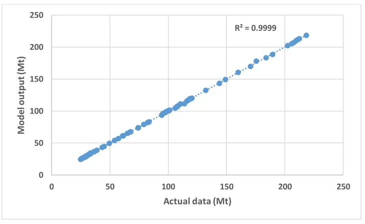
consumptions. In order to assess the model’s precision, some statistical criteria are used [26]. In

comparing the actual data and the outputs of the obtained model reveals that this value is 0.9999.

This value is very close to 1, which means high accuracy of the proposed regression.

Figure 9 Actual data vs model's outputs in the case of applying GMDH

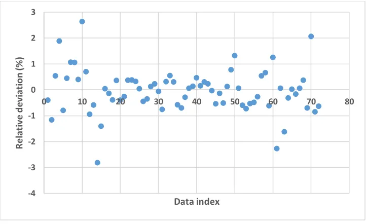
Another criterion used for evaluation is the absolute relative deviation. Based on this criterion, the

model can accurately forecast the emission of carbon dioxide, which can be attributed to both

model ability and appropriateness of the selected input variables. According to Figure 10, the

highest absolute relative deviation of the obtained model is approximately 2.81%, which is another

indicator of the model’s acceptable accuracy. Moreover, the average absolute relative deviation of

this model is about 0.61%. It should be mentioned that since the data are divided into two subsets

in the case of using ANN, which are randomly used for train the network and test, the data indexes

are different from the correlation.

R² = 0.9999

0 50 100 150 200 250

0 50 100 150 200 250

M

o

d

el

o

u

tp

u

t (M

t)

Figure 10 Relative deviation of model's outputs in the case of applying GMDH

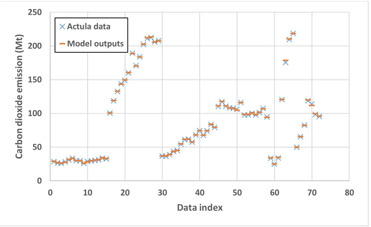
In order to gain more appropriate insight into the model outputs, the actual data and corresponded

model outputs are compared in Figure 11. As it can be observed, the data are in the close vicinity

of each other. In the majority of the cases, the data obtained by the regression and actual data are

approximately equal. Therefore, it can be concluded the model is very reliable to predict carbon

dioxide emission and analyze the share of each input variable on it. By applying this model,

production of carbon dioxide in the investigated countries can be accurately estimated for different

scenarios in future years.

-4 -3 -2 -1 0 1 2 3

0 10 20 30 40 50 60 70 80

R

el

at

iv

e

d

ev

ia

ti

o

n

(%

)

Figure 11 Comparison between model outputs and actual data in the case of applying GMDH

4. Conclusion

The emission of carbon dioxide depends on several factors such as share of energy sources in total

primary energy consumption and the economic activities. In this paper, four CIS countries

including Uzbekistan, Turkmenistan, Azerbaijan and Kazakhstan, are considered as cases of the

study to model the carbon dioxide production on the basis of GDP, as an economic indicator, and

consumption of various fuels and renewable energies. The employed methods for modeling are

linear correlation and GMDH ANN. The R-squared values obtained by the correlation and

ANN-based model are 0.9997 and 0.9999, respectively. In addition, the average absolute relative

deviations in out the cases of using the correlation and GMDH are about 1.05% and 0.61%,

respectively. It is concluded that using GMDH in modeling the emission of carbon dioxide results

in more precise estimation.

References

[1] Rezaei MH, Sadeghzadeh M, Alhuyi Nazari M, Ahmadi MH, Astaraei FR. Applying

GMDH artificial neural network in modeling CO2 emissions in four nordic countries. Int J

0 50 100 150 200 250

0 10 20 30 40 50 60 70 80

C

arb

o

n

d

io

xi

d

e

em

is

si

o

n

(M

t)

Data index

Actula data

Low-Carbon Technol 2018. doi:10.1093/ijlct/cty026.

[2] Dehghani Madvar M, Alhuyi Nazari M, Tabe Arjmand J, Aslani A, Ghasempour R, Ahmadi

MH. Analysis of stakeholder roles and the challenges of solar energy utilization in Iran. Int

J Low-Carbon Technol 2018;13:438–51. doi:10.1093/ijlct/cty044.

[3] BP Statistical Review of World Energy. 2018.

[4] Ahmadi MH, Ahmadi MA, Sadaghiani MS, Ghazvini M, Shahriar S, Alhuyi Nazari M.

Ground source heat pump carbon emissions and ground-source heat pump systems for

heating and cooling of buildings: A review. Environ Prog Sustain Energy 2017.

doi:10.1002/ep.12802.

[5] Mirzaei M, Ahmadi MH, Mobin M, Nazari MA, Alayi R. Energy, exergy and economics

analysis of an ORC working with several fluids and utilizes smelting furnace gases as heat

source. Therm Sci Eng Prog 2018;5:230–7. doi:10.1016/j.tsep.2017.11.011.

[6] Russell A, Ghalaieny M, Gazdiyeva B, Zhumabayeva S, Kurmanbayeva A, Akhmetov KK,

et al. A Spatial Survey of Environmental Indicators for Kazakhstan: An Examination of

Current Conditions and Future Needs. Int J Environ Res 2018;12:735–48.

doi:10.1007/s41742-018-0134-7.

[7] Ramezanizadeh M, Nazari MA, Ahmadi MH, Lorenzini G, Kumar R, Jilte R. A review on

the solar applications of thermosyphons n.d. doi:10.18280/mmep.050401.

[8] Ahmadi MH, Ramezanizadeh M, Nazari MA, Lorenzini G, Kumar R, Jilte R. Applications

of nanofluids in geothermal: A review. Math Model Eng Probl 2018;5:281–5.

[9] Alhuyi Nazari M, Aslani A, Ghasempour R. Analysis of Solar Farm Site Selection Based

on TOPSIS Approach. Int J Soc Ecol Sustain Dev 2018;9.

[10] Álvarez P, Pérez L, Salgueiro JL, Cancela Á, Sánchez Á, Ortiz L. Bioenergy Use from

Pavlova lutheri Microalgae. Int J Environ Res 2017;11:281–9.

doi:10.1007/s41742-017-0026-2.

[11] Dębowski M, Zieliński M, Kisielewska M, Krzemieniewski M. Anaerobic Co-digestion of

the Energy Crop Sida hermaphrodita and Microalgae Biomass for Enhanced Biogas

Production. Int J Environ Res 2017;11:243–50. doi:10.1007/s41742-017-0024-4.

[12] Ramezanizadeh M, Alhuyi Nazari M, Ahmadi MH, Açıkkalp E. Application of nanofluids

in thermosyphons: A review. J Mol Liq 2018;272. doi:10.1016/j.molliq.2018.09.101.

[13] Ahmadi MH, Alhuyi Nazari M, Ghasempour R, Pourfayaz F, Rahimzadeh M, Ming T. A

review on solar-assisted gas turbines. Energy Sci Eng 2018. doi:10.1002/ese3.238.

[14] Ahmadi MH, Ahmadi MA, Nazari MA, Mahian O, Ghasempour R. A proposed model to

predict thermal conductivity ratio of Al2O3/EG nanofluid by applying least squares support

vector machine (LSSVM) and genetic algorithm as a connectionist approach. J Therm Anal

Calorim 2018:1–11. doi:10.1007/s10973-018-7035-z.

[15] Ahmadi MH, Tatar A, Alhuyi Nazari M, Ghasempour R, Chamkha AJ, Yan W-M.

Applicability of connectionist methods to predict thermal resistance of pulsating heat pipes

with ethanol by using neural networks. Int J Heat Mass Transf 2018;126:1079–86.

doi:10.1016/j.ijheatmasstransfer.2018.06.085.

application of machine learning methods to predict the heat transfer performance of

CNT/water nanofluid flows through coils. Int J Heat Mass Transf 2019;128:825–35.

doi:10.1016/J.IJHEATMASSTRANSFER.2018.09.041.

[17] Toghyani S, Ahmadi MH, Kasaeian A, Mohammadi AH. Artificial neural network,

ANN-PSO and ANN-ICA for modelling the Stirling engine. Int J Ambient Energy 2016;37:456–

68. doi:10.1080/01430750.2014.986289.

[18] Maddah H, Aghayari R, Ahmadi MH, Rahimzadeh M, Ghasemi N. Prediction and modeling

of MWCNT/Carbon (60/40)/SAE 10 W 40/SAE 85 W 90(50/50) nanofluid viscosity using

artificial neural network (ANN) and self-organizing map (SOM). J Therm Anal Calorim

2018;1. doi:10.1007/s10973-018-7827-1.

[19] Ahmadi MH, Ahmadi MA, Ashouri M, Razie Astaraei F, Ghasempour R, Aloui F.

Prediction of performance of Stirling engine using least squares support machine technique.

Mech Ind 2016;17:506. doi:10.1051/meca/2015098.

[20] Kahani M, Ahmadi MH, Tatar A, Sadeghzadeh M. Development of multilayer perceptron

artificial neural network (MLP-ANN) and least square support vector machine (LSSVM)

models to predict Nusselt number and pressure drop of TiO 2 /water nanofluid flows through

non-straight pathways. Numer Heat Transf Part A Appl 2018:1–17.

doi:10.1080/10407782.2018.1523597.

[21] Ahmadi MH, Hajizadeh F, Rahimzadeh M, Shafii MB, Chamkha AJ. Application GMDH

artificial neural network for modeling of Al 2 O 3 / water and Al 2 O 3 / Ethylene glycol

thermal conductivity 2018;36:773–82.

a 25W fabricated PEM fuel cell by parametric and GMDH-type neural network. Mech Ind

2016;17:105. doi:10.1051/meca/2015050.

[23] Loni R, Asli-Ardeh EA, Ghobadian B, Ahmadi MH, Bellos E. GMDH modeling and

experimental investigation of thermal performance enhancement of hemispherical cavity

receiver using MWCNT/oil nanofluid. Sol Energy 2018;171:790–803.

doi:10.1016/J.SOLENER.2018.07.003.

[24] Ivakhnenko AG. The group method of data handling- a rival of the method of stochastic

approximation. Sov Autom Control 1966;13:43–55.

[25] www.forestresearch.gov.uk n.d.

[26] Alver A, Baştürk E, Kılıç A. Disinfection By-Products Formation Potential Along the

Melendiz River, Turkey; Associated Water Quality Parameters and Non-Linear Prediction