The Study Of The Method Of The Direct Torque Control Based On Space Vector Pulse Width Modulation

(1)

1

The Study of the Method of the Direct

Torque Control Based On Space Vector

Pulse Width Modulation

Ruan Shihao, LIU Weiting,Wei Haifeng,Yan Pengyu,Yao Jinyi,Chen Jiaqi

School of Electrical and Information, Jiangsu University of Science and Technology, Zhenjiang 212003, China

Abstract：The paper expounds the mathematical

model of permanent magnet synchronous motor,

which introduces the general principle of the direct

torque control and the space vector pulse width

modulation. In the MATLAB/simulink environment,

the mathematical model of permanent magnet

synchronous motor sets up a simulation model of the

direct torque control which based on the theory of

SVPWM. Each step and process of the simulation

model is introduced in detail and finally the

simulation result is obtained. The simulation result

shows that the direct torque control system which

based on the theory of SVPWM has a constant switch

frequency, can reduce the torque ripple greatly, and

improves the current waveform and flux linkage

waveform. So it makes the system have a better

dynamic and static performance and also verify the

feasibility and effectiveness of the plan.

Key words: Permanent magnet synchronous motor;

Direct torque control; SVPWM

0

INTRODUCTION

With the rapid development of power

electronics technology, motor speed regulation

theory and microelectronics technology, as

well as the continuous change and update of

permanent magnet material, the frequency

control technology of Permanent Magnet

Synchronous Motor has been into the rapid

development stage. Permanent Magnet

Synchronous Motor are attaining more and

more attention due to its simple structure, high

moment of inertia ratio, high energy density,

high efficiency, high power, low loss, good

maintainability and so on. Simultaneously,

PMSM has been widely applied into areas of

industrial robots, machining centers, electric

traction, CNC machine tools and aerospaceP

[1]

P

.

The traditional direct torque control

method takes advantage of the hysteresis

control. The width is restricted by the

frequency of inverter switching, which

requires that during one control cycle time,

there is only one basic voltage vector working,

so it will result in the flux and torque ripple

and other issues. Meanwhile, for the SVPWM

control, it can synthesize any desired voltage

vector, which is able to reduce flux linkage

and torque ripple obviously, in order to

improve the system's dynamic static

performance. This paper introduces the direct

torque control program of PMSM on the base

of SVPWM, and makes a stimulation study on

SIMLINK.

1 Mathematical model of PMSM

Make the following assumptions for

convenient analysis before building

mathematical model:

①Ignore the effect of core saturation,

eddy current and hysteresis;

(2)

2 damping winding;

③The three-phase stator winding is

completely symmetrical, and the axes of the

winding of each phase are spatially different

from each other by 120 °. The armature

resistances and inductance of the stator

winding are equal;

④Induced electromotive force (EMF)

and air gap magnetic field are distributed

along the sine, and regardless of the impact of

higher harmonics of the magnetic field.

There are A, B and C three-phase

winding on the stator. There are excitation winding f and direct-axis damping winding D

on the straight shaft of the rotor, and cross-axis damping winding Q on the cross shaftP

[2]

P

. The schematic diagram is shown in

Figure1.1.

Figure 1.1 synchronous motor schematic

Based on the above assumptions, mathematical model of three-phase a, b, c

stationary coordinate system of PMSM rotor magnetic field:

Stator voltage equation is:

    

+ =

c

s

ca

b

s

b

a

s

a

p i R u

ψ ψ

ψ

(1-1) a

u

,

u

b_,

u

c_{are instantaneous value of stator}

winding voltage;

i

a _,

i

b _,

i

c _are

instantaneous value of stator winding phase

current;

ψ

a _,

ψ

b _,

ψ

c _{are instantaneous}

flux value;

p

is differential operator,

;

R

s _{is stator armature phase}

resistance.

Electromagnetic torque equation:

    

  

     

− +

− =

3 4 sin sinθ θ π

ψ_f _a _b

p

e n i i T

(1-2)

e

T

refers to permanent magnet

synchronous motor electromagnetic torque;

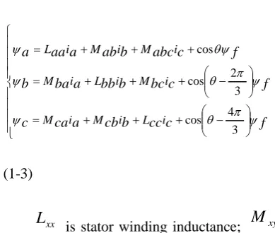
Stator flux equation:

          

     

− + + +

=

     

− + +

+ =

+ +

+ =

f c

cc b cb a ca c

f c

bc b bb a ba b

f c

abc b ab a aa a

i L i M i M

i M i L i M

i M i M i L

ψ π θ ψ

θψ ψ

3 4 cos

3 2 cos

cos

(1-3)

xx

L

is stator winding inductance;

M

xy

is mutual inductance between stator winding;

xy represents one of abc's;

ψ

f_{is rotor flux}

linkage;

θ

is the electrical angle between the

rotor axis and the a-axis.

Based on the above assumptions, the

mathematical model of PMSM rotor magnetic field in two-phase stationary coordinate

(3)

3 system:

Stator voltage equation:

   

+ +

+ =

− +

+ =

θ ωψ

α

αβ

β

αβ

α

sin sin

ψ

α

i

β

ψ

β

i

α

)

n

T_e = _p −

2 3

(1-6)

α

u

,

u

β are the

αβ

axis component

of the stator voltage vector;

R

s _{is stator}

armature phase resistance;

θ

is electrical

angle of the rotor axis to the a axis;

i

α,

i

β

are the

αβ

axis component of the stator

current vector;

p

is differential operator,

dt

d

p

[3]

P

.

2 Traditional DTC control strategy

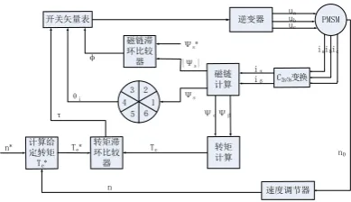
2.1 The basic principle of direct torque control

The principle of the traditional DTC

control scheme is shown in Figure 2.1.1

逆变器 ua

ub

uc

iaibic

ΨαΨβ

iα

iβ

n0

n Te

PMSM

计算给定转矩 Te*

-n*

C2s/3s变换

转矩计算 Te*

磁链计算 Ψs*

|Ψs|

Ψs

速度调节器 1

2 3 4

5 6 φ

θi

τ

磁链滞环比较器

转矩滞环比较器开关矢量表

Figure 2.1.1 PMSM direct torque control system

schematic

The traditional idea of DTC control is to select the appropriate voltage vector by

querying the way of vector switch table to realize the direct control of flux linkage and torque. (The switch voltage vector table

shown in Table 1.) Traditional direct torque control scheme is established in the two-phase

stationary coordinates

αβ

. First of all,

measure the terminal voltage and the terminal

current of the motor; then the transform the coordinate; that is to say, switch the

three-phase stationary coordinate system into the two-phase stationary coordinate system. Use formula (1-5) to calculate the stator flux

s

ψ

, and use formula (1-6) to calculate the

electromagnetic torque

T

e_{, and determine the}

sector in which the flux is located, as shown in

Figure 2.1.2 stator flux vector trajectory.

Compare the given flux linkage

*

s

(4)

4 torque

*

e

T

with the calculated flux linkage

s

ψ

and torque

T

e_{respectively. Get into}

the hysteresis comparator to control the error. Through the two quantities of the error value

and the sector value , you can choose the appropriate voltage space vector, in order to

achieve the motor flux and torque direct

controlP

[4]

P

.

Table 1 switch voltage vector selection table

ψ

∆

_∆

_T

Ⅰ Ⅱ Ⅲ Ⅳ Ⅴ Ⅵ

1

1 U6 U2 U3 U1 U5 U4

0 U5 U4 U6 U2 U3 U1

0

1 U2 U3 U1 U5 U4 U6

0 U1 U5 U4 U6 U2 U3

2.2 Direct Torque Control Simulation Experiment

Motor direct torque control is divided into coordinate transformation module, torque,

flux estimation module, and hysteresis comparison and switching voltage meter selection module. Under the Simulink

simulation environment of MATLAB, the system simulation model of DTC-based

permanent magnet synchronous motor is established according to the control principle of DTC, as shown in Figure 2.2.1.

In the simulation experiment, the parameters of permanent magnet synchronous motor are set as follows: the given motor

speed is 100r/min, the sampling period

T

s

=1e-005s, the simulation time of MATLAB is 0.2s, the DC bus voltage is Udc=310V. At 0.05s plus step load 1N·m, pole pairs number

p

_{=2, stator resistance}

R

s =20.51Ω, the

given value of stator flux

*

s

ψ

_=0.8wb,

cross-axis inductance

L

d _=0.168H,

direct-axis inductance

L

q _{=0.168H, torque}

inertia J=0.0008kg·m2

100 w

Discrete, Ts = 1e-005 s.

powergui

fluxalpha fluxbeta angle ||

figure out angle angleSn figure out Sn

XY Graph1

U_abc U_a U_b V3/2 g A B C + -Universal Bridge

Vabc Iabc A B C a b c Three-Phase V-I Measurement w*

w Te* Te* caculator

ia cia ib cib Te Te caculator

Sector SF STe

pulse Sa Sb Sc

ia ua ib ub cia

cib Subsystem

Step

Scope6

Scope2

Scope1

Scope 0.8

Q* Tm

m A B C Permanent Magnet Synchronous Machine

I_abc I_a I_b I3/2

2 Gain3

DC

<Stator current is_a (A)> <Stator current is_b (A)> <Stator current is_c (A)> <Electromagnetic torque Te (N*m)> <Rotor speed wm (rad/s)>

is_abc

Figure 2.2.1 Permanent Magnet Synchronous Motor

Direct Torque System Simulation Model

3 SVM-DTC control strategy

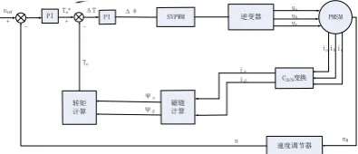
3.1 SVM-DTC control principle

The principle of SVM-DTC control

scheme is shown in Figure 3.1.1

PI PI SVPWM

C2s/3s变换

磁链计算转矩

计算

逆变器

速度调节器

nref ua

ub uc +

- +

-iaibic

Ψα Ψβ

iα iβ

n0 n

Te

PMSM

t

Te* ΔT Δθ

Figure 3.1.1 SVM-DTC control schematic

Compared with the traditional direct torque control scheme, SVM-DTC scheme uses the PI regulator instead of the traditional

scheme of torque hysteresis comparator and flux hysteresis comparator. In addition,

SVPWM module instead of the query switch table. In the control strategy of SVM-DTC, the motor will issue multiple voltage vectors

according to the error of torque and flux linkage in arbitrary control cycle, so as to

(5)

5 flux linkage, reduce the torque ripple, and let

the output waveform become smoother, which in order to obtain better dynamic performance

and static performanceP

[5]

P

.

α

U1 U2

U3 U4

U5 U6

β

Ⅲ

Ⅱ

Ⅰ

Ⅵ

Ⅴ Ⅳ

Uref

θ T6 TsU6

T4 TsU4

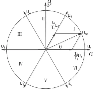
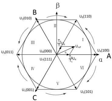
Figure 3.1.3 Basic space voltage vector diagram

Space vector pulse width modulation technology works by using the adjacent two

basic voltage space vector of different action time, as shown in Figure 3.1.3. In the figure, I, II, III, IV, V, VI indicate the sector number

where the reference voltage vector

U

ref_is

located.

U

0_,

U

7_{is zero voltage vector,}

U

1

~

U

6_{is the effective basic voltage vector.}

And these eight basic voltage space vector can

be any number of different voltage space vector synthesis, so that each cycle can choose a reasonable voltage space vector to

compensate for the error of motor torque and stator flux between the observations and

reference valuesP

[6]

P

. In order to be able to

compensate for the error

∆

T

e_{between the}

observed torque value

T

e_{and the torque}

reference output

T

ref _{of the speed regulator,}

it can take advantage of the PI regulator to

calculate the phase angle

∆

θ

, the reference

vector

ψ

ref _{of the flux linkage, the flux}

observation value

ψ

s_{and the phase angle}

s ψ

θ

of the observation value, which stator

flux required to be added, and then get into the flux compensation module to calculate the flux component of the compensation value

α

ψ

S

∆

and

∆

diagram shown in Figure 3.1.2

磁链补偿值分量的计算

电压空间矢量计算

θ

∆ s

ψ

θ

re f

ψ

s

ψ

ref

U_α

ref

U_β SVM 驱动信号 PI

e

T +

-e

T ∆ *

e

T

α

ψ

_S

∆

∆ψSβ

Figure 3.1.2 SVPM module schematic

(6)

6

β

α

θ

Δθ

re f

ψ

∆

ψ

s

ψ

Figure 3.2.1 Stator flux vector

Permanent magnet synchronous motor stator flux vector diagram in Figure 3.2.1, in

which

ψ

s_{is the reference value of stator}

flux vector,

ψ

ref _{is the reference value of}

stator flux vector ,

∆

ψ

s_{is the compensation}

value of stator flux ,

ψ

f _{is the flux vector of}

rotor permanent magnet,

θ

is the angle of

the stator flux vector observations and

∆

θ

is

the increased angle of stator flux vector phase angle.

The calculation process of reference

voltage vector is as follows:

Magnetic chain compensation equation:

(

)

(

)









−

∆

+

=

∆

−

∆

+

=

∆

θ

ψ

θ

ψ

θ

ψ

θ

ψ

β α

sin

s ref

S

s ref

S

(3-1)

Reference voltage space vector equation：

      

+ ∆ =

+ ∆

=

β β

β

α α

α

ψ ψ

i R T U

i R T

U

s s S ref

(3-2)

Stator flux vector equation:

    

+ =

β

α

θ ψ

ψ

θ ψ

ψ

i L

s

ref

S

s

ref

S

sin cos

(3-3)

In the three-phase inverter circuit, it is assumed that the conduction of the power

switch is 1 and the cutoff is 0, we can get the 8

switch status (000 ~ 111) of power switchP

[7]

P

. And the corresponding inverter will output 6

vector is 60°, and the diameter of a hexagon inscribed circle consisting of vector vertices is

dc

U

3

1

.

α

U1(001)

U2(010)

U3(011) U4(100)

U5(101)

U6(110)

β

A

B

U0(000)

U7(111)

C

Ⅲ

Ⅱ

Ⅰ

Ⅵ

Ⅴ Ⅳ

Uref

θ

T6

TsU6

T4

TsU4

Figure 3.2.2 Reference voltage space vector synthesis

diagram

As shown in the above figure, take the

the reference voltage vector

U

ref_{in the first}

(7)

7

ref

U

≤

1

3 U

dc_{, then}

U

ref _{is within the}

inscribed circle. Therefore,

U

ref _{can be}

synthesized by voltage vector

U

4_{and zero}

vector

U

6_{. At the same time, define}

T

₄_，

6

T

_，

T

0_{as the operating time of}

U

₄_，

U

6

and zero voltage vector in a cycle period,

T

s

is the sampling period of system.

In a sampling period, the calculation process of the reference voltage vector in the adjacent two basic voltage vector of the action

time

T

4_,

T

6_{is shown as follows:}

Take Ⅰ sector as an example, according

to the principle of volt-second balance, the relationship between the reference voltage

vector

U

ref _{and the basic voltage vector}

4

U

_is:

(

₄ ₄ ₆ ₆

)

1 _T _U _T _U

T U

s

ref = + (3-4)

0 0 6 6 4

4U T U T U T

T_s = + + _(3-5)

Map the voltage vector to

α

，

β

axis,

shown in figure 3.2.2, and according to the formula (3-4)(3-5), we can get

      = + = 3 sin 3 cos

6

4

π π

β

α

U T T U U T U T T U

s

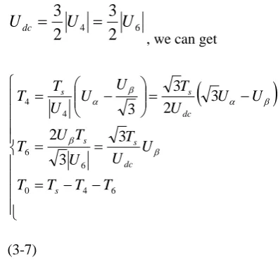
(3-6)

according to formula (3-5) (3-6), and

6 4

2

3

2

3 U

U

_dc

=

, we can get

(

)

          − − = = = − =       − = 6 4 0 6 6 4 4 3 3 2 3 2 3 3 T T T T U U T U T U T U U U T U U U T T s dc s s dc s s β β β α β α (3-7)

Among them, when T4 + T6> T, that is

saturated status, then 4 6

4 4

T

s

+

∗

=

， 6 4 6 6

T

s

+

∗

=

.

Through the previously calculated size of

ref

U

_α

，

U

βref_{, you can determine the sector}

position of spatial voltage reference vector, the operating process is as follows:

U

ref

sin

θ

_{, When}

ref

U

is in sector I, the condition is true

0 >

β

U

，

3 tan

π

α β

_<

U

，that is,

    > − > 0 3 0

β

α

β

U U U (3-8)

In other sectors，we can get three

intermediate variables

M

1，

M

2，

M

3_through

(8)

8

of the same method, and

M

1，

M

2，

M

3

are：

    

    

 

   



₋ ₋

=

   



 ₋

= =

β

α

β

α

β

U U U

T M

U U U

T M

U U

T M

dc

s

dc

s

dc

s

3 2

3 3 2

3 3

3

2

1

(3-9)

Defining variable a, b, c. If

M

1_>0，_then

a=1，or a=0；if

M

2_{>0 , then b=1}，_{or b=0}；

if

M

3_>0_，_{then c=1}_，_{or c=0. Afterwards,}

defining N=4c+2b+a，then N=1~7，We

need to define them one by one，thus, we can

judge the sector position due to N value, and

then get the table 3-1.

Tab.3-1 The relationship between sector position

and N.

N 1 2 3 4 5 6

sectors Ⅱ Ⅵ Ⅰ Ⅳ Ⅲ Ⅴ

After determine the sector position of

ref

U

, we need to Use equation (3-7) to

calculate the individual action time

T

4，

T

6

P

[8]

P

.

The following section describes the

relationship between sector position and action time:

Define variable X，Y，Z；

    

    

 

   



₋ ₊

=

   



 ₊

= =

β

α

β

α

β

U U U

T Z

U U U

T Y

U U

T X

dc s dc s dc s

3 2

3 3 2

3 3

(3-10)

According to equation (3-7), we can get the relationship between T4, T6 and the

sectors, as shown in Table 3-2:

Tab.3-2 Duration of voltage vectors in each sector

sect

ors Ⅰ Ⅱ Ⅲ Ⅳ Ⅴ Ⅵ

T4 -Z Z X -X -Y Y

T6 X Y -Y Z -Z -X

After determining the operating time of a sector and the corresponding space voltage

vector, We can calculate the value of each corresponding comparator according to PWM modulation principle, and the operation

process is as follows:

Defining the the comparison points of

trigger pulse PWM1，PWM3，PWM5 as

1

cmp

T

，

T

cmp2_，

T

cmp3_{. At the same time, define}

three intermediate variables

T

a_，

T

b_，

T

c_{, and}

their values is

(

)

  

   

 

+ =

− − =

6

4

6

4

2 1 2 1 4 1

T T T

T T

T

T T T T

b

c

a

b

a

(3-11)

(9)

9 sectors and comparison points, as shown in

Table 3-3.

Tab. 3-3 Computation of Switch Switching Point

Values

sect

ors Ⅰ Ⅱ Ⅲ Ⅳ Ⅴ Ⅵ

1

cmp3_{, and the triangular}

wave to get the SVPWM output timing.

3.3 SVPWM control simulation experiment

Under the Simulink simulation environment of MATLAB, the system

simulation model of permanent magnet synchronous motor based on SVM-DTC is established according to the control principle

of SVPWM, as shown in Figure 3.3.1. The main structure of SVM-DTC control system

of permanent magnet synchronous motor includes the calculation of reference voltage

vector

U

ref _{, the module simulation model is}

shown in Figure 3.3.2; The judgment of sector

ref

U

, the module simulation model is shown

in Figure 3.3.3. The operating time of effective voltage vector and zero voltage vector, the module simulation model shown in

Figure 3.3.4. Time allocation of changing

switch, the module simulation model shown in

Figure 3.3.5.

In the simulation experiment, the

parameters of permanent magnet synchronous motor are set as follows: the given motor

speed is 100r/min, the sampling period is

T

s

=1e-005s, the simulation time of MATLAB is

0.2s, the bus voltage of DC is Udc=310V, In 0.05s, plus step load is 1N·m, the number of

pole pairs is

p

=2, the stator resistance is

s

R

_{=20.51Ω, the set point of Stator flux is}

ref

ψ

=0.8wb, the cross-axis inductance is

d

L

=0.168H, the direct-axis inductance is

L

q

=0.168H, the torque inertia is J=0.0008kg·m2.

U_abc u_ahpa u_beta u3/2

Discrete, Ts = 2e-005 s.

powergui

Iabc I_ahpa I_beta i3/2 ialpha ibeta ualpha ubeta Rs fluxalpha fluxbeta |flux| jiao figure out fluxalpha fluxbeta ialpha

ibeta fluxalpha fluxbeta Np Te

figure out Te

g A B C + -Universal Bridge

Vabc Iabc A B C a b c Three-Phase V-I Measurement Deta

flux* theta_s flux i_beta i_alpha g Sa Sb Sc Subsystem

Step1 Scope4

Scope2

Scope1

Scope Tm

m A B C Permanent Magnet Synchronous Machine I O

PI1 I O PI

2 Gain3 0.8

Flux*

DC 100

Constant3

10 Constant2 2

Constant1

<Stator current is_a> <Stator current is_b> <Stator current is_c > <Rotor speed wm >

is_abc <Electromagnetic torque Te>

Figure 3.3.1 Permanent magnet synchronous motor

SVM-DTC simulation model

beta *

4Sc

3Sb

2Sa

1g

sin

Trigonometric Function3

cos Trigonometric

Function2 cos Trigonometric

Function1 sin Trigonometric

Function

u_beta

u_alfa pulse

Sa

Sb

Sc

Subsystem

10 Rs

Product7 Product6 Product3

Product2

Product1 Product

Divide1 Divide

0.0002 Constant3

0.0002 Constant2

Add4 Add3 Add2

Add1 Add

|u| Abs1 |u|

Abs 6

i_alpha 5 i_beta

4 flux 3 theta_s

2 flux* 1 Deta

Figure 3.3.2 Calculation of voltage space reference

(10)

10

1 N

Switch2 Switch1 Switch

4 Gain1 2 Gain

f(u) Fcn3 f(u)

Fcn2 f(u) Fcn1 u(2) Fcn

0 Constant1

1 Constant

2 ubetar

1 uaphar

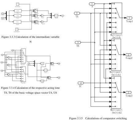
Figure 3.3.3 Calculation of the intermediate variable

N

2 T6 1

Switch1 Switch

Multiport Switch1 Multiport Switch

-1 Gain2 -1 Gain1

-1 Gain

f(u) Fcn2

f(u) Fcn1 Fcn -C

Constant

4 Z 3 Y 2 X

1 N

f(u)

T4

Figure 3.3.4 Calculation of the respective acting time

T4, T6 of the basic voltage space vector U4, U6 3

Tcmp3 2 Tcmp2

1 Tcmp1

Multiport Switch2 Multiport Switch1 Multiport

Switch

4 TC 3 TB 2 TA

1 N

Figure 3.3.5 Calculations of comparator switching

points Tcpm1，Tcmp2，Tcmp3

4 Simulation results of DTC and

SVM-DTC control strategy

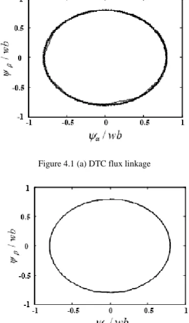
Simulation and experimental results are shown in Figure 4.1 ~ Figure 4.4. Figure 4.1 shows the stator flux trajectory under two

control schemes. Observing Fig. 4.1 (a) and Fig. 4.1 (b), in both cases the flux trajectories

are approximately circular, but in comparison, the flux trajectory under the SVM-DTC scheme is smoother and the flux linkage

Fluctuations are obviously small. This shows that the use of SVM-DTC program greatly

enhances the overall system steady-state

performanceP

[9]

P

(11)

11 Figure 4.1 (a) DTC flux linkage

Figure 4.1 (b) SVM-DTC flux trajectory

Figure 4.2 shows the stator phase current

waveform. By comparing Fig. 4.1 (a) and Fig. 4.1 (b), it can be concluded that the start-up current is large and the steady state time is

long when the traditional DTC scheme is adopted. However, the stator current of the

motor adopting SVM-DTC scheme starts smoothly, the amount of modulation is small , the time achieving steady state is short, and

the waveform is closer to the sine wave. And in the SVM-DTC scheme, the stator current is

sinusoidal and the current ripple is less than 0.1A.

is_abc/A

-6 -4 -2 0 2 4 6

0 0.02 0.04 0.06 0.08 0.1 0.12 0.14 0.16 0.18 0.2 t/s

Figure 4.2 (a) DTC stator three-phase current

is_abc/A

-3 -2 -1 0 1 2 3 4

0.2 0 0.02 0.04 0.06 0.08 0.1 0.12 0.14 0.16 0.18

t/s

Figure 4.2 (b) SVM DTC stator three-phase current

Figure 4.3 (a) and Figure 4.3 (b) show

the electromagnetic torque waveform at steady state. Under the two schemes, the speed of the motor is 0 N·m, at the beginning, and the step

load torque is increased by 1N·m at 0.05s. Comparing Figure 4.3 (a) with Figure 4.3 (b),

we can see that when the motor is started, the torque waveform of the traditional DTC scheme fluctuates greatly and the torque

waveform response time is longer. In the SVM-DTC control scheme, the torque quickly responds to the change of the load torque, that

is, the dynamic response of the system is rapid and the overshoot is small with no static error

in the steady stateP

[10]

P

.

This shows that the motor has good

system performance under SVM-DTC control strategy and the motor can output more stable

and accurate torque.

Te/(N*m)

-10 -5 0 5 10 15

0 0.02 0.04 0.06 0.08 0.1 0.12 0.14 0.16 0.18 t/s

Figure 4.3 (a) DTC torque waveform

-4 -2 0 2 4 6 8

Te /(N*m)

0.2 0 0.02 0.04 0.06 0.08_t/s 0.1 0.12 0.14 0.16 0.18

Figure 4.3 (b) SVM-DTC torque waveform

Figure 4.4 shows the motor speed

(12)

12 Comparing Figure 4.4 (a) and Figure 4.4 (b),

we can find that the speed response time of the system adopting SVM-DTC control scheme is

shorter. When the load changes from zero to 1N.m at 0.05s, the speed is controlled by a certain overshoot, but it quickly stabilizes well.

The system using the traditional DTC control scheme, the speed response time is longer, and

when the load torque changes, the speed will

fluctuate significantlyP

[11]

P

.

-100 -50 0 50 100

0 0.02 0.04 0.06 0.08 0.1 0.12 0.14 0.16 0.18 0.2 t/s

ω/(rad/s)

Figure 4.4 (a) DTC speed waveform

ω/(rad/s)

0 10 20 30 40 50 60

0.2 0 0.02 0.04 0.06 0.08 _t/s 0.1 0.12 0.14 0.16 0.18

Figure 4.4 (b) SVM-DTC speed waveform

5 Conclusion

From the simulation results in this paper, we can see that in the traditional DTC control strategy, the current, torque and flux ripple are

large, and the static dynamic performance is not particularly stable. But the space voltage

vector modulation technology, which takes advantage of SVM, use voltage vector to completely compensate the stator flux error,

and make use of the PI regulator to replace the traditional hysteresis comparator in order to

achieve steady-state flux-free no-static control. Thus it can reduce the flux ripple and torque ripple of the motor, which is able to make the

flux locus smoother and the electromagnetic torque tracking faster. Also, the advantage of

fast response in the traditional DTC control

scheme is maintained.

References and Notes

[1] Steimel A. Direct self-control and

synchronous pulse techniques for

high-power traction inverters in comparison[J].

IEEE Trans Ind Electro，2004，51(4)：810-820.

[2] Giuseppe S，Buja Marian，P Kazmierkowski.

Direct Torque Control of PWM Inverter-Fed AC

Motors-A Survey[J]. IEEE Trans Ind

Electronics，2004，51(4)：744-757.

[3] Song Jianguo，Chen Quanshi. Research of

Electric Vehicle IM Controller Based On Space

Vector Modulation Direct Torque Control. 8th

ICEMS 2005：1617-1620.

[4] Jin Mengjia，Shi Cenwei，Qiu Jianqi，et

al. Stator Flux Estimation for Direct

Torque Controlled Surface Mounted

Permanent Magnet Synchronous Motor

Drives over Wide Speed Region. ICEMS，

2005：350-354.

[5] Tripathi A ， Khambadkone A M ，

Panda S K. Torque ripple analysis

and dynamic performance of a space vector

modulation based control method for AC-drives.

IEEE Trans Power Electronics，2005：485-492.

[6] Parsa L，Toliyat H A. Sensorless direct

torque control of five-phase interior

permanent magnet motor drives. 39th IAS，

(13)

13

[7] Dan Sun，Yikang He，Zhu J G.

Sensorless direct torque control for

permanent magnet synchronous motor based on

fuzzy logic. 4th IPEMC，2004，3：1286-1291.

[8] Linni Jian，Liming Shi. Stability Analysis for

Direct Torque Control of Permanent Magnet

Synchronous Motors. 8th ICEMS 2005

1672-1675.

[9] Linni Jian，Liming Shi. Stability Analysis for

Direct Torque Control of Permanent Magnet

Synchronous Motors. 8th ICEMS 2005

1672-1675.

[10] Yen-Shin Lai ， Fu-San shyu ， Yung-Hsin

Chang. Novel Loss Reduction

Pulsewidth Modulation Technique for

Brushless dc Motor Drives Fed by

MOSFET Inverter[J]. IEEE Trans on Power

Electronics，2004，19(6)：1646-1652.

[11] Yong Liu，Z Q Zhu，David Howe.

Direct Torque Control of Brushless DC

Drives With Reduced Torque Ripple[J]. IEEE