R E S E A R C H
Open Access
Performance characterization and
transmission schemes for instantly decodable
network coding in wireless broadcast
Mingchao Yu
*, Parastoo Sadeghi and Neda Aboutorab
Abstract
We consider broadcasting a block of packets to multiple wireless receivers under random packet erasures using instantly decodable network coding (IDNC). The sender first broadcasts each packet uncoded once, then generates coded packets according to receivers’ feedback about their missing packets. We focus on strict IDNC (S-IDNC), where each coded packet includes at most one missing packet of every receiver. But, we will also study its relation with generalized IDNC (G-IDNC), where this condition is relaxed. We characterize two fundamental performance limits of S-IDNC: (1) the number of transmissions to complete the broadcast, which measures throughput and (2) average packet decoding delay, which measures how fast each packet is decoded at each receiver on average. We derive a closed-form expression for the expected minimum number of transmissions in terms of the number of packets and receivers and the erasure probability. We prove that it is NP-hard to minimize the average packet decoding delay of S-IDNC. We also prove that the graph models of S- and G-IDNC share the same chromatic number. Next, we design efficient S-IDNC transmission schemes and coding algorithms with full/intermittent receiver feedback. We present simulation results to corroborate the developed theory and compare our schemes with existing ones.
Keywords: Wireless broadcast, Network coding, Throughput, Packet decoding delay, Feedback
1 Introduction
The broadcast nature of wireless medium allows one sender to simultaneously serve multiple receivers who are interested in the same data. We consider a block-based wireless broadcast system where a sender wishes to deliver a block of data packets to a set of receivers. The chan-nels between the sender and the receivers are subject to independent random packet erasures. In such systems, a traditional approach is to retransmit the data packets under a receiver feedback mechanism, such as Automatic-Repeat-reQuest (ARQ) [1]. This approach, though simple, is inefficient in terms of throughput, as the transmit-ted packets are non-innovative to the receivers who have already received them.
The advent of network coding (NC) [2] starts a new era for high-throughput network coded wireless com-munications [3–17]. By linearly adding all data packets
*Correspondence: [email protected]
Research School of Engineering, Australian National University, Canberra, Australia
together with randomly chosen coefficients from a suf-ficiently large finite field, random linear network coding (RLNC) can almost surely achieve the minimum block completion time [9–11, 18], which is defined as the num-ber of transmissions it takes to complete the broadcast. Due to the inverse relation between block completion time and throughput under a fixed block size, RLNC can almost surely achieve optimal throughput.
However, with RLNC, data packets are block-decoded by solving a set of linear equations, which can only take place after a sufficient number of coded packets have been received. RLNC thus may suffer from high decoding computational load [11], as well as large average packet decoding delay (APDD) [16], which reflects how fast each data packet is decoded at each receiver on average. High decoding computational load may not be afford-able by receivers with limited computational and energy resources, such as mobile and sensor receivers [11]. Large APDD is undesirable in applications where individual data packets are useful, such as image transmissions and video streaming [19–21].
To alleviate decoding computational load and APDD, the sender can transmit all the data packets uncoded once at the beginning of the broadcast. This method allows the receivers to directly obtain a subset of data pack-ets. It is also throughput optimal and constitutes the systematic transmission phase of RLNC [11]. But in the subsequentcoded transmission phase, RLNC still requires block decoding and suffers from high decoding computa-tional load and APDD.
To further mitigate these issues in the coded transmission phase, instantly decodable network coding (IDNC) techniques [3, 12–15] have been introduced. They make online coding decisions based on receivers’ feedback about their packet reception state, under the restriction that coding/decoding is over the binary field. In other words, IDNC techniques shift the computational load to the sender, and allow receivers to perform sim-ple binary XOR based instant packet decodings, as the sender (such as a base station) usually has much more computational and energy resources than the receivers.
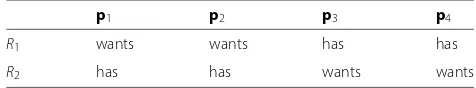
For a handy example of IDNC techniques, consider the packet reception state in Table 1. There are 4 data pack-ets,p1,2,3,4, and 2 receivers,R1,2.R1has receivedp3,4and only wantsp1,2, whileR2has receivedp1,2and only wants p3,4. Consider two IDNC coded packetsX1=p1⊕p3and X2 = p2⊕p4, where⊕denotes the binary XOR oper-ator. By transmittingX1andX2and assuming no packet erasures, both receivers can instantly decode one wanted data packet after each transmission. Hence, there are two data packets decoded in the first transmission and two data packets decoded in the second transmission. The cor-responding APDD is1+1+42+2 =1.5. In contrast, if RLNC is applied, all data packets are decoded after the second transmission, yielding an APDD of 2.
We also note from the above example that an IDNC coded packet ofX=p1⊕p2⊕p3is not instantly decod-able toR1. Restrictions on such packets separate IDNC techniques into two variations. The first one, called strict IDNC (S-IDNC) [13–15], prohibits the transmissions of non-instantly decodable packets to any receiver. Effec-tively, each coded packet can include at most one wanted data packet of every receiver. The second one, called gen-eralized IDNC (G-IDNC), removes this restriction for more coding opportunities.
Therefore, S-IDNC can be thought of as a sub-class of G-IDNC, in the sense that every valid S-IDNC coded packet is also a valid G-IDNC coded packet.
Table 1A example of packet reception state
p1 p2 p3 p4
R1 wants wants has has
R2 has has wants wants
Although G-IDNC has been extensively studied under various wireless broadcast settings, including basic ones [12, 12, 22–28] and those with limited/lossy feedback [29, 30] or with hard deadline [31], most developed algorithms are heuristics, leaving the optimal G-IDNC in terms of throughput and APDD still unknown or intractable due to prohibitively large computational com-plexity. Hence in this paper, we take a step back, aiming to understand the performance limits and optimal imple-mentations of a sub-class of G-IDNC, namely, S-IDNC. This will facilitate the applications of S-IDNC, while also providing new insights into the more general G-IDNC class.
So far, studies on theoretical performance characteri-zation and implementations of S-IDNC have been quite limited in both breath and depth. S-IDNC was graphically modeled in [13], which then proved that the minimum clique partition solution [13] of the associated graph can be an S-IDNC solution that minimizes the block com-pletion time. However, this solution does not take into account the issues of decoding delay and the robustness of coded transmissions to erasures. S-IDNC has shown to be asymptotically throughput optimal when there are up to three receivers or when the number of data packets approaches infinity [20], but the general relation between the throughput of S-IDNC and system parameters has not been characterized before. In addition and to the best of our knowledge, the minimum packet decoding delay of S-IDNC is still unknown. Moreover, there have not been S-IDNC transmission schemes that can work with inter-mittent receiver feedback. Another unaddressed problem is a systematic performance comparison between S-IDNC and G-IDNC.
In this paper, we study the above problems and provide the following contributions:
1. We characterize the throughput performance limits of S-IDNC. Specifically, we derive a closed-form expression for the expected minimum block completion time in terms of the number of packets and receivers and their erasure probabilities. 2. We prove that it is NP-hard to minimize the APDD
of S-IDNC. We derive an upper bound on the minimum packet decoding delay in terms of the minimum block completion time.
4. We also provide new results on the relation between S-IDNC and G-IDNC. For example, we prove the equivalence between the chromatic number of S- and G-IDNC graphs.
2 System model and notations
2.1 Transmission setup
We consider a block-based wireless broadcast scenario, in which the sender needs to deliver a block ofKdata pack-ets, denoted byPK = {pk}Kk=1, toNreceivers, denoted by RN = {Rn}Nn=1through wireless channels that are subject
to independent random packet erasures.
Initially, the K data packets are transmitted uncoded once usingK time slots, constituting asystematic trans-mission phase[11]. Then, each receiver provides feedback to the sender about the packets it has received.1The com-plete packet reception state is represented by anN ×K state feedback matrix (SFM)A, wherean,k = 0 ifRnhas
already receivedpk, andan,k = 1 ifRn has missed (and
thus still wants)pk. The set of data packets wanted byRn
is called theWantsset ofRnand is denoted byWn. The set
of receivers who wantpkis called theTargetset ofpkand
is denoted byTk. The size ofTkis denoted byTk. Packets
with largerTkare more desired by receivers.
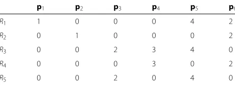
Example 1.Consider the SFM in Fig. 1a with K = 6 data packets and N = 5receivers. The Wants set of R1is
W1 = {p1,p5,p6}. The Target set ofp3isT3 = {R3,R5} and thus T3=2.
Then based onA, the sender starts the second phase, called thecoded transmission phase, in which coded pack-ets are transmitted until the broadcast is completed, i.e, until all receivers have recovered all theKdata packets. A sketch of the two-phase transmission scheme is plotted in Fig. 2.
2.2 Coded transmission phase: two types of IDNC In the coded transmission phase, the sender generates IDNC coded packets under the binary fieldF2. Explicitly,
IDNC coded packets are of the form X = pk∈Mpk,
whereMis a selected subset ofPK, and is called an IDNC coding set. There are three possible types of decodability ofXat each receiver:
Definition 1.1. An IDNC coded packetX is instantly decodable for receiver Rn ifMcontains exactly one data
packet from the Wants setWnof Rn, i.e., if|M∩Wn| =1.
Definition 1.2.An IDNC coded packet X is non-instantly decodable for receiver Rn ifMcontains two or
more data packets from the Wants set Wn of Rn, i.e., if |M∩Wn|>1.
Definition 1.3.An IDNC coded packet X is non-innovative for receiver Rn ifMcontains no data packets
from the Wants set Wn of Rn, i.e., if |M ∩Wn| = 0.
Otherwise, it is innovative.
Restrictions on the above three types of packet decod-ability separate IDNC into two variations. The first one is called strict IDNC (S-IDNC), which is the main subject of our study. It prohibits the transmission of any non-instantly decodable coded packets to any receiver. This restriction implies that any two data packets wanted by the same receiver cannot be coded together. We thus have the concept of conflicting and non-conflicting data packets:
Definition 2.Two data packetspi andpjconflict if at
least one receiver wants both of them, i.e., if∃n:{pi,pj} ⊆ Wn. Otherwise they do no conflict.
An S-IDNC coding set is thus a set of pairwise non-conflicting data packets. The non-conflicting state between all data packets can be represented by an undirected graph
Gs(V,E). Each vertexvi ∈ V represents a data packetpi.
Two verticesviandvjare connected by an edgeei,j ∈Eif piandpjdo not conflict. Thus, every complete subgraph
ofGs, a.k.a., a clique, represents an S-IDNC coding set. In the rest of the paper, we will use the terms “coded packet”,
Fig. 2The considered two-phase transmission schemes. Receiver feedback must be collected by the end of the systematic transmission phase (solid arrow). Intermediate feedback during the coded transmission phase (dashed arrows) are optional
“coding set”, and “clique” interchangeably, and denote the last two byM.
The main limitation of S-IDNC is that a coded packet which is instantly decodable for a large subset of receivers may be prohibited because it is non-instantly decodable for a small subset of receivers. In the second type of IDNC, called generalized IDNC (G-IDNC), the restriction on non-instantly decodable packets is removed for more coding opportunities.2
G-IDNC can also be graphically modeled [23]. The difference is that, in the G-IDNC graph Gg(V,E), a data packet pk wanted by different receivers are individually
represented by different verticesvn,k, for allan,k =1.
Con-sequently, the number of vertices in Gg is equal to the number of “1”s inA. Two verticesvm,i andvn,j are
con-nected by an edge if: (1)i =j, or (2) ifpi ∈/ Wnandpj ∈/ Wm. In the first case,pi=pj, and thus by sendingpiboth
RmandRncan decode. In the second case, by sendingpi⊕ pj,RmandRncan decodepiandpj, respectively, because
they already have pj and pi, respectively. Similar to
S-IDNC, every clique of Gg represents a G-IDNC coding set.
We note that an S-IDNC coded packet is always a G-IDNC coded packet, but the reverse is not necessar-ily true. Below is an example of S- and G-IDNC coded packets.
Example 2.Consider the SFM and its S- and G-IDNC graphs in Fig. 1. The G-G-IDNC graph indicates that (v1,1,v5,3,v4,4)is a clique. The corresponding G-IDNC cod-ing set is (p1,p3,p4), and thus Xg = p1 ⊕ p3 ⊕ p4
is a G-IDNC coded packet. Xg is instantly decodable
for R1,R4,R5 because they only want one data packet from Xg. Xg is non-instantly decodable for R3 because R3 wants both p3 and p4. Xg is non-innovative for
R2.
Due to the existence of R3, Xg is not an S-IDNC
coded packet. Whereas the S-IDNC graph indicates that (v1,v2,v3) is a clique. The corresponding coding set is (p1,p2,p3), and thusXs = p1⊕p2⊕p3 is an S-IDNC
coded packet, which can be verified to also correspond to clique(v1,1,v2,2,v3,3,v5,3)in the G-IDNC graph.
We then introduce the notion of IDNC solution. A set of IDNC coding sets is called an IDNC solution if, upon the reception of the coded packets of all these coding sets, every receiver can decode all its wanted data packets. An S-IDNC solution is denoted by Ss. The set of all S-IDNC solutions of a given SFM is denoted bySs. Similarly, we can also defineSgandSgfor
G-IDNC.
For the SFM in Fig. 1, by partitioning the S-IDNC graph into three disjoint cliques, we can obtain, among others, an S-IDNC solution with three cliques/coding sets: Ss = {(p1,p4),(p2,p5),(p3,p6)}. We can also partition the S-IDNC graph into four disjoint cliques and obtain Ss = {(p1,p2,p3),p4,p5,p6}. Similarly, a disjoint clique partition of the G-IDNC graph is
{(v1,1,v2,2,v5,3,v4,4), (v3,3,v1,6,v2,6,v4,6), (v1,5,v3,5,v5,5), (v3,4,v4,4)}, indicating a G-IDNC solution of Sg =
{(p1,p2,p3,p4),(p3,p6),(p5),(p4)}.
To assess the performance of IDNC solutions, we now introduce our measures of throughput and decoding delay.
2.3 Throughput and decoding delay measures
An S-IDNC solutionSsrequires a minimum of|Ss|coded transmissions. We call USs |Ss| the minimum block completion timeofSs. It measures the best throughput of
Ss, because the total number of transmissions in the sys-tematic and coded transmission phases is lower bounded by K + U§s, yielding a throughput of
K
K+U§s packet per
transmission. We further denote byUsthe absolute
mini-mum block completion time over all the S-IDNC solutions ofA, i.e.,Usmin{U§s :§s∈Ss}. Similarly, we denote by Ugthe absolute minimum block completion time over all
the G-IDNC solutions ofA.
(APDD)D, which is the average time it takes for a receiver to decode a data packet. For example, the APDD of all receivers is calculated as:
the minimum APDD ofS. We further denote byDs(resp.
Dg) the absolute minimum APDD over all S- (resp. G-)
IDNC solutions ofA. We also note that in the specific case of an S-IDNC solutionSs,un,kis indeed the index of the
first coding set in Ss that containspk, as every receiver
who wantspkcan decode it from this coding set.
Example 3.Consider the SFM in Fig. 1a. Suppose that an S-IDNC solution with four coded packetsX1=p1⊕p2, X2= p3⊕p6,X3= p4, andX4 =p5are transmitted in this order. The receivers’ decoding time{un,k}are
summa-rized in Table 2. The minimum APDD of this solution is DSs =(1×2+2×5+3×2+4×3)/12=2.5.
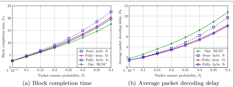
In each time slot of the coded transmission phase, the sender selects and broadcasts a coding set through erasure-prone wireless channels. We denote by UT the
block completion time of the coded transmission phase, and byDTthe APDD of this phase, calculated as in (1).UT
andDT measure the throughput and decoding delay
per-formance of this phase, respectively. They vary according to the IDNC solutions, transmission schemes, and erasure patterns. But it always holds thatUT UsandDT Ds
if S-IDNC is applied. Therefore, Us and Ds reflect the
performance limits of S-IDNC. Hence, we will first study these limits in the next section, and then design S-IDNC transmission schemes and coding algorithms in Sections 4 and 5, respectively.
3 Performance limits and properties of IDNC In this section, we study performance limits and proper-ties of S-IDNC and compare it with G-IDNC.
Table 2The decoding delay of original data packets at the receivers
3.1 Absolute minimum block completion timeUs
We first study the throughput limit of S-IDNC, measured by the absolute minimum block completion timeUs. It has
been proved thatUsis equal to the size of the minimum
clique partition solution3ofGs[13], denoted bySc. This equivalence holds because of the following property:
Property 1.Removing any vertex from the S-IDNC graph does not change the connectivity of the remaining vertices.
This property holds because vertices inGsrepresent dif-ferent data packets. Thus, to remove all vertices fromGs (i.e., to complete the broadcast), at least|Sc|cliques must be removed, which yieldsUs= |Sc|.
According to graph theory,|Sc|is equal to the chromatic number4χ(Gs) of the complementary graphGs, which has the same vertex set asGs, but has opposite vertex connec-tivity. We thus have Us = χ(Gs). Bounds and
approxi-mations on the chromatic number of a given graph have been well-studied in the graph theory literature [33–35]. They provide some insights into theUs of a given SFM.
In this subsection, we are interested in the probabilistic characterization ofUs, asGs is the consequence of
ran-dom packet erasures in the systematic transmission phase. Specifically, we address the following question:what is the relation between Usand system parameters, including the
number of data packets and receivers, as well as the packet erasure probability?
For wireless broadcast, a common assumption on ran-dom packet erasures is that they are independently and Bernoulli distributed at each receiverRn with an erasure
probability ofPe,n. Under this assumption, a similar
ques-tion has already been introduced and answered for the RLNC technique. RLNC has been proved to be asymptot-ically throughput-optimal, for each RLNC coded packet is almost surely linearly independent of the previous RLNC coded packet(s) when the finite field is sufficiently large [11]. Hence, RLNC is able to offer the smallest block com-pletion time among all NC techniques. It has also been shown in [6, 36, 37] that the block completion time of RLNC scales asO(ln(N))whenK is a constant. Conse-quently, the throughput of RLNC vanishes with increasing number of receivers N. To prevent zero throughput, it has been proved in [38] that K should scale faster than ln(N).
Theorem 1.The mean of the absolute minimum block completion time Us is a function of the block size K, the
number of receivers N, and packet erasure probability
{Pe,n}Nn=1:
where o(1) is a small term that approaches zero with increasing K.
Proof. Our approach is to model the complementary S-IDNC graph Gs after the systematic phase as a random graph with i.i.d. edge generating probability. Recall that two vertices inGsare connected if the two data packets conflict, i.e., if at least one receiver has missed both pack-ets. Therefore, the generating probability of every edge, denoted byPc, is calculated as:
Pc=1− N
n=1
1−Pe2,n. (3)
Then, the key is to prove that different edges are gen-erated independently. We first consider the independence between two adjacent edges. Without loss of generality let us consider the generation ofe1,2 ande1,3, two edges that are adjacent via v1, and are incident to v2 andv3, respectively. We denote byP(e1,2)the probability thate1,2 is generated. It holds thatP(e1,2)=P(e1,3)=Pcin (3). We
further denote byP(e1,2|v1)the probability thate1,2is gen-erated conditioned on thatv1is generated. We then argue the following relations:
1. P(e1,2,v1)=P(e1,2), because the generating ofe1,2 already indicates thatv1is generated. Similarly, we also haveP(e1,3,v1)=P(e1,3);
2. P(v1|e1,2,e1,3)=1because of the same reason as above;
3. P(e1,e2|v1)=P(e1|v1)·P(e2|v1), because ifv1is already generated, the generating ofe1(resp.e2) only depends on whetherp2(resp.p3) is wanted by some of the receivers who wantp1. Since wantingp2and p3are independent events for every receiver, the generating ofe1ande2is independent conditioned on thatv1is generated;
4. P(v1)2≈P(v1)≈1, and the accuracy increases quickly with increasing number of receiversN. This is becauseP(v1)is the probability that at least one receiver has missedp1in the systematic transmission phase. It has a value of1−Nn=1(1−Pe,n), which
quickly approaches to 1 with increasingN.
Then, to prove thate1,2ande1,3are generated indepen-dently, we only need to show thatP(e1,2,e1,3) = P(e1,2)·
where (4) follows Bayes’ rule. Hence, the generation ofe1,2 ande1,3are asymptotically independent of each other.
On the the other hand, it is intuitive that two disjoint edges in Gs are generated independently. Therefore, we can assume that all edges in Gs are generated indepen-dently.
Consequently, Gs can be modeled as an Erdõs-Rényi random graph [39], which hasK vertices and i.i.d. edge generating probability ofPc. Figure 3 compares the mean
number of edges (with a value ofK(K−1)/2·Pc) of our
proposed random graph model and the simulated aver-age number of edges inGs. Our model shows virtually no deviation under all considered values ofNandK.
From graph theory, givenK andPc, almost every
ran-dom graphGshas a chromatic number of [40]:
χ(Gs)= K
substituting (3) into (5) we obtain (2).
Theorem 1 has the following important corollary:
Corollary 1.The mean E[Us]of the absolute minimum
block completion time of S-IDNC increases almost linearly with the number of receivers when all receivers experience similar packet erasure probabilities.
Proof. This corollary can be proved by letting
{Pe,n}Nn=1 = Pe, which will transform (2) into a linear
Then, by noting that the mean block completion time of the coded transmission phase is lower bounded byE[Us],
Fig. 3The mean and simulated number of edges inGswhen{Pe,n}Nn=1=0.2 andK∈[20, 100]
reduce decoding delay [41]. In the next subsection, we will study the APDD of S-IDNC.
3.2 Absolute minimum average packet decoding delayDs Unlike Us, to the best of our knowledge, there is no
existing hardness result on findingDs. In this subsection,
we address it through the following theorem and then propose an upper bound onDs.
Theorem 2.It is NP-hard to find the absolute minimum
APDD Dsof S-IDNC.
In order to prove it, we first reveal the perfect decoding scenario of each receiver. We first note that it is impossible for a receiver to decode more thanuwanted data pack-ets from the firstucoded packets, for anyu > 0. Then for every receiverRn, its perfect decoding scenario is to
decode one of its|Wn|wanted data packet from each of the first|Wn|coded packets. Intuitively, this scenario min-imizes both the BCC and APDD experienced byRn. By
extending the perfect decoding scenario to all receivers, we obtain the concept ofperfect S-IDNC solution:
Definition 3.An S-IDNC solution is perfect and is denoted bySp if every receiver Rn can decode one of its |Wn| wanted data packets from each of the first |Wn| coding sets inSp.
By its definition,Spoffers the perfect packet decoding scenario for all receivers; every coded packet allows all receivers that are still missing data packets to decode one
wanted data packet. Therefore, its APDD, denoted byDSp,
is a lower bound ofDs, and can only be achieved if Sp
exists. The value ofDSpis:
DSp =
1 T
N
n=1
wn
i=1
i. (7)
The hardness of deciding the existence ofSp is as fol-lows:
Theorem 3.It is NP-complete to decide the existence of
Spfor a given SFM.
It is proved through a reduction from a graph γ -colorability (γ 3) problem, which is well-known to be NP-complete [34]. The proof is given in Appendix 1. Then by noting thatDSpcan only be achieved bySp, Theorem 3 has the following corollary:
Corollary 2.It is NP-complete to decide the achievabil-ity of DSpfor a given SFM.
Corollary 2 proves Theorem 2 by contradiction; if it is easy to find Ds for a given SFM, then we can
eas-ily decide the achievability ofDSp by comparingDswith DSp, as Ds = DSp means that DSp is achievable, and Ds>DSpmeans thatDSpis not achievable. However, this
result contradicts with Corollary 2. Hence, it is NP-hard to findDs.
Property 2.The absolute minimum APDD Dsis upper
decode a data packet fromMu. The minimum APDD of
Ssis thus:
2 . Applying this result to an S-IDNC solution with absolute minimum block completion timeU = Us,
we obtain the result.
Our proof indicates that, although it is NP-hard to achieveDs, we can still effectively reduce APDD by
reduc-ing the sizes of our S-IDNC solutions. Before we further explore this result to implement S-IDNC, we would like to compare the performance limits of S-IDNC that we have just derived with G-IDNC.
3.3 S-IDNC vs. G-IDNC
In this subsection, we address the question ofhow does S-IDNC compare with G-IDNC?
We first note that the NP-hardness of finding Ds
also holds for Dg. This is because the perfect
S-IDNC solution Sp is also the best possible G-IDNC solution. For the throughput, we first present a rela-tion between S- and G-IDNC graphs (proved in the appendix):
Theorem 4. The minimum clique partition solutions of S-IDNC and G-IDNC graphs have the same size. In other words,χ(Gs)=χ(Gg).
This theorem, together with Corollary 1, indicates that χ(Gg) also increases almost linearly with N when all receivers experience similar erasure probabilities. How-ever, the above theorem does not implyUs =Ug. This is
because G-IDNC does not have Property 1. Explicitly, by removing a vertex fromGg, more edges and larger cliques may be generated, and thus the absolute minimum block completion timeUgcan be smaller thanχ(Gg)of the
orig-inal G-IDNC graphGg [24]. We thus haveUg Us. We
note, however, that a systematic way of findingUg other
than brute-force search remains widely open.
4 S-IDNC transmission schemes
In this section, we design S-IDNC transmission schemes to compensate for packet erasures in the coded transmis-sion phase. To this end, the sender has to regularly collect feedback from the receivers about their packet recep-tion state to make online coding decisions. We consider transmission schemes with two different types of feedback frequency, namely:
1. Fully-online feedback: feedback is collected after every coded transmission. However, this could be costly in wireless communications. We thus also consider a reduced feedback frequency next;
2. Semi-online feedback: feedback is only collected after transmitting a complete S-IDNC solution;
To be able to design S-IDNC transmission schemes, two questions need to be answered first:
1. What is the optimization objective for throughput and decoding delay improvement?
2. What does the sender need to send to achieve it?
Before addressing these questions, we first highlight some challenges:
Remark 1.Under random packet erasures, a reason-able measure of throughput is the mean block completion time E[UT]of the coded transmission phase. However, it
is intractable to minimize E[UT]. To see this, let us
con-sider the stochastic shortest path (SSP) method [23]. In SSP method, the state space comprises the current SFM and its successors, and thus has a prohibitively large size with a value of2T, where T is the number of “1”s inA. The action
space for each state comprises all cliques/coding sets, which is NP-hard to find [42]. Then, E[UT]is recursively
min-imized by examining all the states and the associated actions. Such examination is necessary, because the packet erasures can take any pattern and are not predictable. But it makes E[UT]intractable to minimize. To overcome this
difficulty, we will turn to optimization objectives that are heuristic, but still based on SSP optimization principles.
Remark 2. It is intractable to minimize the APDD DT
of the coded transmission phase due to the NP-hardness of finding Ds, because otherwise by setting Pe = 0, the
min-imum DT is equal to Ds. To overcome this difficulty, we
simulations, which show that DT generally decreases with
decreasing UT.
4.1 Fully-online transmission scheme
In this scheme, the current state in SSP is the cur-rent SFM A, the absorbing state is the all-zero SFM and is denoted by A0. The action space comprises all the S-IDNC coding sets of A. The cost of each action is one, for it consumes one transmission. The block completion timeUT is thus equal to the number
of transitions (a.k.a. path length or distance) between AandA0.
According to Remark 1, it is intractable to choose an action/coded packet that minimizes the expected path length (and thus E[UT]). As a heuristic alternative, we
propose to choose an action/coded packet that belongs to the shortest path from A to A0, which has a length of Us. This choice guarantees that, upon the reception
of the coded packet at all interested receivers, the short-est distance between the updated state A and A0 is minimized to Us − 1. To this end, the coded packet
must belong to a minimum clique partition solutionSc. Otherwise, the shortest distance between A and A0 is stillUs.
We then reduce APDD by forcing the coded packet to be maximal (and thus serving the maximal number of receivers). However, cliques in a minimum clique par-tition solution are not necessarily maximal. Hence, we further require the coded packet to belong to a set of Usmaximal cliques that together cover all the data
pack-ets. This set is also an S-IDNC solution and is denoted bySm.
In conclusion, we propose the following coded packet
Mf for fully-online transmission scheme:
Given an SFM instance, the preferred coded packetMf is the most wanted coded packet inSm, whereSm is an S-IDNC solution that contains Usmaximal cliques.
4.2 Semi-online transmission scheme
The current and absorbing states in this scheme is the same as in the fully-online scheme. But the action space becomes the set of all S-IDNC solutions Ss, and the
cost of each action is the solution size |Ss|, which is equal to the length of a semi-online transmission round. The total cost is thus equal to the block completion time.
According to Remark 1, it is intractable to minimize the expected total cost (and thusE[UT]). As a heuristic
alternative, we propose to minimize the expected cost of the shortest path between AandA0. The shortest path includes only one transition, representing the event that every coded packet of the chosen solutionSsis received by all the interested receivers after only one semi-online
round. Denote the probability of this event byPs. Then the
expected cost is|Ss|/Ps, wherePsis calculated as:
Here,dk is called the packet multiplicity and is defined
below.
Definition 4.The multiplicity dkof data packetpkis the
number of coding sets inSsthat comprisepk.
We note that the minimum clique partition solutionSc is not a preferred semi-online S-IDNC solution. Although
Scoffers the smallest solution size (|Sc| =Us), it does not
maximizePsbecause every data packet has a multiplicity
of only one due to disjoint cliques inSc. In contrast, the
Sm we have proposed for the fully-online case can offer a higherPsthanScdue to possibly overlapping maximal
cliques, while also offering the smallest solution size. We still wish to answer the following question before choosingSmas our preferred semi-online S-IDNC solu-tion: Is there a solution that, though is large in its size, provides higher packet multiplicities, so that Ps is
maxi-mized?
An explicit answer to this question is difficult to obtain, because it requires the examination of all the solutions of size greater thanUs. Such search is costly and does not
provide any insight into this question. Moreover, a larger solution is unlikely to provide higher packet multiplicities due to the following property of S-IDNC solutions:
Property 3.Every coding set in an S-IDNC solution comprises at least one data packet with a multiplicity of one.
This property holds because if every data packet in a coding set has a multiplicity of greater than one, then this coding set can be removed from the solution with-out affecting the completeness of the solution. Due to the above property, an S-IDNC solutionSs has at least|Ss| data packets with a multiplicity of only one. According to (10), these unit-multiplicity data packets reducePsthe
most. Hence, S-IDNC solutions with a larger size may have more unit-multiplicity data packets than Sm, and thus are not preferable.
Therefore, we chooseSmfor throughput improvement. Then, by taking into account our secondary optimization objective, i.e., the APDD, we define our preferred semi-online S-IDNC solution as follows:
Given an SFM instance, the preferred semi-online S-IDNC solution isSm, which comprises a set of Usmaximal
A flow-chart of the proposed two transmission schemes are presented in Fig. 4. Both the fully- and semi-online IDNC schemes require findingSm. Since packet multiplic-ity is not a concern in graph theory, algorithms that find
Smdo not exist in the graph theory literature. Hence, we will design algorithms dedicated for S-IDNC in the next section. Before moving on, we briefly compare S-IDNC and G-IDNC under the above two transmission schemes.
4.3 S-IDNC vs. G-IDNC
With fully-online feedback, the sender can update the G-IDNC graphGg and add new edges representing coding opportunities after every transmission. The throughput of G-IDNC is thus better than S-IDNC. But, the price is high computational load, because G-IDNC graph is much larger than S-IDNC graph (O(NK) vs. O(K)). On the other hand, it has been proved in [30] that, when receiver feedback is not available, the best strategy for the sender is not to updateGg (compared with certain probabilistic update strategy). Therefore, during a semi-online trans-mission round, the sender only sends the minimum clique partition solution ofGg, which, according to Theorem 4, has the same size as the minimum clique partition solu-tion of S-IDNC.
5 S-IDNC coding algorithms
The two transmission schemes we proposed in the last section require findingSm, an S-IDNC solution that con-tainsUsmaximal coding sets. In this section, we develop
its optimal and heuristic algorithms.
5.1 Optimal S-IDNC coding algorithm
Our optimal algorithm finds all validSmin two steps:
Step-1 Find all the maximal coding sets (maximal cliques): This problem is NP-hard in graph theory [42], and thus cannot be optimally solved by an algorithm whose computational
complexity is a polynomial of the numberK of data packets. However, it can be solved by
exponential algorithms such as Bron-Kerbosch (B-K) algorithm [42]. We use B-K algorithm to optimally find the group of all maximal cliques and denote the group byA.
Step-2 Find all validSmfromA: We propose a branching algorithm in Algorithm 1. The intuition behind this algorithm is that, if a data packetpkbelongs todkmaximal coding sets in A, then one of thesedkmaximal coding sets must
be included inSmfor the completeness ofSm. In the extreme case wheredk=1, the sole
maximal coding set that containspkmust be
included inSm. Below is an example of Algorithm 1.
Example 4.Consider the graph model in Fig. 5. In Step-1, we find all the maximal cliques:A = {(p1,p3),
(p2,p3,p5),(p3,p4),(p4,p6),(p5,p6)}. Then in Step-2:
1. Initially,S= ∅,S =A\S=A, and the set of data packets not included inSis
P = {p1,p2,p3,p4,p5,p6}. Sincep1is only included in(p1,p3)andp2is only included in(p2,p3,p5), these two coding sets must be added toS. Hence,
S = {(p1,p3),(p2,p3,p5)}after the first two iterations;
2. The set of data packets not included inSis
P = {p4,p6}, and the remaining maximal coding sets areS =A\S={(p3,p4),(p4,p6),(p5,p6)}}. Sincep4 has a multiplicity of 2 underSdue to(p3,p4)and
(p4,p6), we branchSinto two successors:
S1= {(p1,p3),(p2,p3,p5),(p4,p5)}and
S2= {(p1,p3),(p2,p3,p5),(p4,p6)}. SinceS2 contains all data packets and there are no other branching opportunities, the algorithm stops and outputsS2asSm.
B-K algorithm and Algorithm 1 constitute our opti-mal S-IDNC coding algorithm. It is optiopti-mal because it exhaustively finds all the validSm from all the maximal
Algorithm 1Optimal S-IDNC solution search 1: input:the group of all maximal coding sets,A; 2: initialization:a setBof solutions,Bonly contains an
empty solutionS= ∅. A counteru=1;
3: whileno solution inBcontains all data packets,do 4: whilethere is a solution inBwith sizeu−1,do 5: Denote this solution byS = {M1,· · ·,Mu−1}.
Denote the data packets included inS byP = u−1
i=1{Mi}and all data packets not included inS byP =PK \P. Also denote the maximal coding sets not included inSbyS =A\S;
6: Pick fromPthe data packetpthat has the small-est multiplicitydunderS. Denote thedcoding sets which containpbyM1,· · ·,Md;
7: BranchSintodnew solutions,S1,· · ·,Sd. Then, add M1,· · ·,Md to these solutions, respec-tively. The sizes of the new solutions areu; 8: end while
9: u=u+1;
10: end while
11: Output the solutions in B that contain all data packets.
coding sets. Among these solutions, we can choose the one that optimizes a secondary criteria, such as the one offering the smallestDS, or the largestPS, calculated using
(10).
5.2 Hybrid S-IDNC coding algorithm
Algorithm 1 is memory demanding, because the number of candidate solutions grows exponentially with branch-ing. Thus, we propose a heuristic alternative to it. The idea is to iteratively maximize the number of data packets included inSm. The algorithm is given in Algorithm 2.
B-K algorithm and Algorithm 2 constitute our hybrid S-IDNC coding algorithm. It produces only one S-IDNC solution, with no guarantee on the solution size. It is still computational expensive due to B-K algorithm. Thus, we develop a polynomial time heuristic S-IDNC coding algorithm next.
Algorithm 2Hybrid S-IDNC solution search 1: input:the group of all maximal coding sets,A; 2: initialization:an empty solutionS = ∅, a counter
u=1, packet setP =PK;
3: whileSdoes not contain all data packets,do
4: find the coding setMinAthat contains the largest number of data packets inP;
5: AddMtoS and remove data packets inMfrom
P;
6: u=u+1;
7: end while
8: Output the solutionS.
5.3 Heuristic S-IDNC coding algorithm
Algorithm 3 is a simple algorithm that heuristically finds the maximum (the largest maximal) clique of a graph. The intuition behind this algorithm is that, a vertex is very likely to be in the maximum clique if it is incident by the largest number of edges. Variations of this algorithm have been developed in the literature [12, 13, 23]. But, this algo-rithm has not been applied to finding a complete S-IDNC solution, and its computational complexity has not been identified yet.
Algorithm 3Heuristic maximum clique search 1: input: graphG(V,E);
2: initialization: an empty vertex setVkeep; 3: whileGis not emptydo
4: add to Vkeep the vertex v which has the largest number of edges incident to it;
5: updateGby deletingvand all the vertices not con-nected to v(These vertices can be ignored because they cannot be part of the target clique, which con-tainsv);
6: end while
7: vertices inVkeepare pair-wise connected, and no other vertices can be added to them. Hence, Vkeep is a maximal clique.
The computational complexity of Algorithm 3 is polynomial in the number of data packetsK. The highest computational cost occurs when the input graph is com-plete, i.e., when all vertices are connected to each other. In this case, only one vertex will be removed in each itera-tion. Thus, the number of remaining vertices in iteration-i will beK−i,∀i∈[0,K−1]. Then, to find the vertex with the largest number of incident edges, we needK−i com-parisons. The total computational cost is thus in the order ofKi=−01K−i=K(K−1)/2. Hence, the computational complexity of Algorithm 3 is at mostO(K2).
We apply Algorithm 3 to iteratively find Sm in Algorithm 4. In each iteration, we find a clique using Algorithm 3, maximize it by adding more vertices to it whenever possible, and then remove it from the S-IDNC graph. This will increase the multiplicities of the added vertices/packets. Below is an example:
Example 5.Consider the graph Gs in Fig. 1b. In the
first two iterations, the algorithm will choose M1 =
(p1,p2,p4)andM2 = (p3,p6), respectively. In the third
Algorithm 4Heuristic S-IDNC solution search 1: input: a graphG(V,E);
2: initialization: an empty vertex setVcovered, a working graphGw=G, and a counteri=0;
3: whileVcovered=Vdo
4: Find the maximum clique inGwusing Algorithm 3. Denote it byMi;
5: Find the vertices inVcoveredwhich are connected to
Mi. Denote their set byVi(They are the candidate vertices that could be added toMi.);
6: Generate a subgraph of G whose vertex set is Vi. Denoted this subgraph byGi(Vi,Ei);
7: Find the maximum clique inGi using Algorithm 1, denoted it byMi(All vertices inMiare connected to each other and thus can all be added toMi.); 8: UpdateVcoveredby adding vertices inMiinto it; 9: UpdateGwby removingMifrom it;
10: UpdateMiasMi = Mi∪Mi(The new clique is at least as large as the old one, and thus provides higher packet multiplicity);
11: i=i+1;
12: end while
In conclusion, we proposed an optimal coding algo-rithm that exhaustively finds all the possibleSm, and also proposed its hybrid and heuristic alternatives. Both the
optimal and hybrid algorithms are exponential-time algo-rithms in terms ofK due to their use of B-K algorithm, while the heuristic algorithm is a polynomial-time one. The output Sm is used as the S-IDNC solution for the semi-online transmission scheme. If fully-online trans-mission scheme is applied, the transmitted coding setMf is chosen fromSm.
6 Simulations
In this section, we present the simulated throughput and decoding delay performance of IDNC (abbreviated as S-in the figures) under different scenarios, S-includS-ing under fully- and semi-online transmission schemes, and under the use of optimal, hybrid and heuristic coding algorithms (abbreviated in the figures as Fully-, Semi-, Opt., Hybr., and Heur., respectively).
We also compare S-IDNC with RLNC and G-IDNC. For RLNC, we assume a sufficiently large finite field, so that its throughput is almost surely optimal and serves as a benchmark. For G-IDNC, although its best perfor-mance is at least as good as S-IDNC (as we have explained in Section 3.3), this advantage will not necessarily be reflected in our simulation results. This is because there has not been any optimal G-IDNC algorithm. Instead, we apply a heuristic algorithm (abbreviated as Heur. G- in the figures) proposed in [23], which aims at minimizing the block completion time. This aim coincides with our opti-mization priorities for S-IDNC in Remark 2, namely, to minimize the block completion time first.
We conduct four sets of simulations. In all simulations we apply a block size ofK=15. In the first three sets, we fixPe=0.2 and set the number of receiversN∈[5and40].
In the fourth set, we fixN=15 and setPe∈[0.05, 0.4].
The purposes of the four sets of simulations are as fol-lows. The first set compares the performance limits of the three techniques. The results are presented in Fig. 6. The second (resp. third) set of simulations compares the throughput and decoding delay performance under fully-online (resp. semi-fully-online) transmission schemes. The results are presented in Fig. 7 (resp. Fig. 8). We note that the performance of RLNC is the same under both schemes, because RLNC is feedback-free. In the fourth set, we evaluate the performance of our hybrid algorithm under different packet erasure probabilities and compare it with fully-online heuristic G-IDNC and RLNC. The results are presented in Fig. 9.
Our observations on S-IDNC are as follows:
• The absolute minimum block completion time of S-IDNC increases almost linearly withN. This result matches Corollary 1;
Fig. 6The throughput and decoding delay performance limits of S- and G-IDNC, and RLNC
• The optimal coding algorithm always provides better throughput performance than its hybrid and heuristic alternatives. This result verifies our choice ofSmfor throughput improvement, because only the optimal coding algorithm can always produceSm, which has
|Sm| =Us;
• However, the optimal coding algorithm does not necessarily minimize the APDD. For example, in Fig. 6b, the hybrid algorithm provides slightly smaller APDD than the optimal one when there are no packet erasures and when the number of receivers isN15;
• The performance gap between the optimal and hybrid algorithms is always marginal, and is much smaller than their gap with the heuristic one. Hence,
the hybrid algorithm strikes a good balance between performance and computational load.
A cross comparison of RLNC, S-, and G-IDNC shows that:
• The throughput of RLNC is always the best. The throughput of S-IDNC is very close to RLNC when the number of receivers is small. Their gap increases withN ;
• In general, the APDD of both S- and G-IDNC is better than RLNC. This advantage only vanishes when the block completion time of S- and G-IDNC becomes much larger than RLNC, which takes place whenN is much larger than K ;
Fig. 8The throughput and decoding delay performance of semi-online transmission scheme when different coding algorithms are applied. It is compared with the performance of heuristic semi-online G-IDNC and RLNC
• With a moderate number of receiversN=15, the APDD of S-IDNC is better than RLNC under all simulated values of packet erasure probability;
• There is no clear winner between the performance of heuristic G-IDNC and optimal S-IDNC. We can expect that G-IDNC will outperform S-IDNC if its optimal coding algorithm is developed.
In summary, our simulations verified our theorems, propositions, and algorithms. They also demonstrated that, if we are concerned with both throughput and decoding delay performance, S-IDNC is a good alterna-tive to RLNC when the number of receivers is not too large.
7 Conclusions
In this paper, we studied the throughput and average packet decoding delay (APDD) performance of S-IDNC in broadcasting a block of data packets to wireless receivers under packet erasures. By using a random graph model, we showed that the throughput of S-IDNC decreases with increasing an number of receivers. By introduc-ing the concept of perfect S-IDNC solution, we proved the NP-hardness of APDD minimization. We derived an upper bound on APDD and showed that minimiz-ing the IDNC solution size can effectively reduce APDD. By applying stochastic shortest path method, we showed that it is intractable to make optimal coding decisions in the presence of random packet erasures. We then
used heuristic objective functions to determine the pre-ferred coded packet(s) to send when fully- or semi-online receiver feedback is collected. We developed optimal and heuristic S-IDNC coding algorithms that minimize the solution size and increase packet multiplicity. We also compared S-IDNC with G-IDNC by proving the equiva-lence between the chromatic number of the complemen-tary S-IDNC and G-IDNC graphs.
Our work provides new understandings of S-IDNC. It will facilitate the extension of S-IDNC to applica-tions in other network settings, such as cooperative data exchange and distributed data storage. We are also inter-ested in designing approximation and heuristic algorithms for APDD minimization.
Endnotes
1We assume that there exists an error-free feedback
link from each receiver to the sender that can be used with an appropriate frequency. The feedback content is the index of the data packets it has received. Each index has a length of log2Kbits. The feedback frequency will be studied in Section 4.
2In traditional G-IDNC, non-instantly decodable
packets will be discarded by the receivers. Storing such packets may further improve throughput with extra computational cost. This problem is beyond the scope of this paper. Interested readers are referred to [32] for a recent treatment.
3The minimum clique partition solution of a graphGis
the minimum set of disjoint cliques ofGthat together cover all the vertices.
4The chromatic number of a graphGis the minimum
number of colors to color the vertices so that any two connected vertices have different colors.
Appendix 1: Proof of Theorem 3
In this appendix we prove that it is NP-complete to decide the existence of the perfect S-IDNC solutionSpfor a given SFMA. Our approach takes two steps: firstly, a polynomial reduction from a graphγ-colorability problem to hyper-graph coloring problem, and then a polynomial reduction from hypergraph coloring problem to our problem of findingSp.
Before we start, we first introduce some related con-cepts and theorems. A graphG(V,E)is calledγ-colorable if there exists a partition of V into γ sets, denoted by
{Vi}γi=1, such that|Vi∩en| 1 for anyen ∈ E. In other
words, vertices inG can be colored using γ colors such that every pair of adjacent vertices have different colors. According to graph theory, it is NP-complete to decide whether a graph G(V,E) is γ-colorable or not for any
γ 3.
A hypergraphHis defined by a set of verticesVand a set of hyperedgesE. Each hyperedgeen ∈E can be incident
to any number of vertices, i.e.,|en| 1.His calledγ
-uniform if every hyperedge is incident toγ vertices, i.e.,
|en| = γ for allen ∈ E.His called stronglyγ-colorable
[43] if there exists a partition ofVintoγ sets, denoted by
{Vi}γi=1, such that|Vi∩en| 1 for anyen ∈ E. In other
words, vertices ofHcan be colored usingγ colors, such that every color appears at most once in every hyperedge. We now prove that it is NP-complete to decide whether aγ-uniform hypergraph is stronglyγ-colorable or not for anyγ 3.
Given anyγ 3 and a graphG(V,E)withK vertices andNedges, we construct a hypergraphH(V,E)as fol-lows: for every edgeen ∈ E, we generate a hyperedgeen
by adding toenγ −2 dummy verticesvn,1· · ·vn,γ−2. The resultedenis incident toγ vertices, whereγ −2 of them are dummy vertices only incident byen. Consequently,H is aγ-uniform hypergraph withK+(γ −2)N vertices. Sinceen⊂enfor alln∈[1,N],Gis a subgraph ofH. Then,
the reduction is as follows:
• IfGisγ-colorable, then for every hyperedgeen, there are already two differently colored vertices. Then, by heuristically color the remainingγ −2dummy vertices inenusing the remainingγ −2colors for all n∈[1,N], we obtain a strongγ−coloring ofH.
• IfHis stronglyγ-colorable, then sinceG⊂H,Gis already colored with at mostγ colors, say with
γ γ colors. To obtain aγ-coloring ofG, we can heuristically chooseγ −γ vertices ofGand assigning each of them with a different new color.
The above reduction indicates that an algorithm that can optimally solve the strong γ-coloring problem for anyγ-uniform hypergraph will also solve theγ-coloring problem of any graph: given any G, we construct Has described above and passHto the algorithm for solution. Then, by noting that it is NP-complete to decide whether G is γ-colorable or not, our reduction proves that it is NP-complete to decide whether a γ-uniform hypergraph is stronglyγ-colorable or not.
We now prove the NP-completeness of deciding the existence ofSpby reducing aγ-uniform hypergraph to a SFMA, and reducing the strongγ-coloring ofHtoSp.
Given anyγ-uniform hypergraphH(V,E) withK ver-tices and N hyperedges, we construct an instance of A with K data packets and N receivers: we identify each vk∈Vwith a data packetpk, and identify eachen∈Ewith
a receiverRnwho wants the data packets represented by
the vertices inen, i.e., lettingWn=en. In the resultingA,
every receiver wantsγ data packets. Then, the reduction is as follows:
• IfHis stronglyγ-colorable, then since everyenhasγ
partition{Vi}γi=1ofVsuch thatVi∩en=1for all
n∈[ 1,n]. Then, by identifying eachViwith a coding setMi, we have|Mi∩Wn| =1. Hence,
S= {Mi}γi=1is a S-IDNC solution that allows all receivers to instantly decode one of theirγ wanted data packets from the coded packet of each of theγ coding sets. According to Definition 3,Sis a perfect S-IDNC solutionSp.
• IfAhas the perfect S-IDNC solutionSp= {Mi}γi=1, then|Mi∩Wn| =1for alln∈[1,N]. Then by identifying eachMiwith a vertex setVi, we obtain a partition{Vi}γi=1ofVsuch that|Vi∩en| =1for all
n∈[1,N]. By definition, this partition is a strong
γ-coloring ofH.
The above reduction indicates that an algorithm that can optimally find the perfect solution for any SFMAwill also solve the strongγ-coloring problem of anyγ-uniform graph: given any such H, we construct an instance of A as described above and pass A to the algorithm for solution.
Then, by noting that it is NP-complete to decide whether aγ-uniform hypergraph is stronglyγ-colorable or not, our reduction proves that it is NP-complete to decide whether the perfect solutionSpexists or not for a givenA.
Appendix 2: Proof of Theorem 4
Theorem 4 requires the proof of χ(Gs) = χ(Gg). Since every S-IDNC solution is also a G-IDNC solution, but a G-IDNC solution is not necessarily an S-IDNC solution, we haveUs Ug, and thusχ(Gs) χ(Gg). Hence, here
we only need to prove thatχ(Gs)χ(Gg).
We first introduce the concept of affiliated S-IDNC graph Gas of a G-IDNC graphGg, which is construct as follows. Given Gg that involves K data packets and N receivers, we generate a graphGas withK vertices, each representing a data packet. We then connect vi and vj
in Gas if for every pair of{m,n} ∈[1,N], vi,m and vj,n
are connected upon their existence inGg. In other words, we claim that pi andpj do not conflict if every vertex
that representspiinGg is connected to every vertex that
representspjinGg.
Given an SFM A, we can easily show that its S-IDNC graphGsis the same as the affiliated S-IDNC graphGasof its G-IDNC graphGg. Hence, our task becomes to prove thatχ(Gas)χ(Gg), whereχ(Gas)=Us. This statement
is true if the following property is true:
After removing any cliqueMg fromGg, the chromatic number of the affiliated S-IDNC graphGasis reduced by at most one.
SinceGg is nonempty as long asGas is nonempty, this property indicates that any clique partition solution of
Gg must have a size of at least χ(Gas), which will prove thatχ(Gas) χ(Gg). Property 6 can be proved through induction:
1. IfMgdoes not contain any conflicting data packets inGas, thenχ(Gas)is reduced by at most one; 2. IfMgcontains one pair of conflicting data packets in
Gas, thenχ(Gs)is reduced by at most one; 3. IfMgalready containsm pairs of conflicting data
packets inGas, then modifyingMgto contain one more pair of conflicting data packets inGascannot further reduceχ(Gas).
The first statement is self-evident, because the set of data packets included in such Mg is a clique of
Gas. By removing it, χ(Gas) can be reduced by at most one.
To prove the second statement, without loss of general-ity we assume that the pair of conflicting data packets is (p1,p2). Then the set of data packets included inMgtakes a form of{Ms,p1,p2}, whereMsis the set of pair-wise non-conflicting data packets, and thus is a clique ofGas. Sincep1conflicts withp2, there exists at least one pair of unconnected vertices inGgthat representsp1andp2. This pair is not included inMg, and thus is kept after remov-ingMgfromGg. Hence, in the updated affiliated S-IDNC graphGas,v1andv2exist, and are unconnected. Let the chromatic number ofGasbeU, then the minimum clique partition ofGas takes a form of {M1,· · ·,MU}, which keepsp1andp2in different coding sets. Then, sinceMs is a clique ofGas,{Ms,M1,· · ·,MU}is a partition ofGas with a size ofU +1. Thus,U χ(Gas)−1, implying thatχ(Gs)is reduced by at most one after removingMg fromGg.
The proof of the third statement is similar to the sec-ond one, and thus is omitted here. According to the above three statements, no matter how many conflicting data packets are included inMg, after removingMgfromGg, the chromatic number of the affiliated S-IDNC graphGas is reduced by at most one. Therefore, χ(Gg) χ(Gas). SinceGas is the same asGs, we haveχ(Gg) χ(Gs)and Theorem 3 is proved.
Competing interests
The authors declare that they have no competing interests.
Received: 29 June 2015 Accepted: 4 November 2015
References
1. JK Sundararajan, D Shah, M Médard, inProc. IEEE Int. Symp. Information Theory (ISIT). ARQ for network coding, (2008)
2. R Ahlswede, N Cai, S Li, R Yeung, Network information flow. IEEE Trans. Inf. Theory.46, 1204–1216 (2000)


![Fig. 3 The mean and simulated number of edges in Gs when {Pe,n}Nn=1 = 0.2 and K ∈ [20, 100]](https://thumb-us.123doks.com/thumbv2/123dok_us/890848.1107176/7.595.58.542.86.308/fig-mean-simulated-number-edges-gs-pe-nn.webp)