Tracking of Multiple Moving Sources
Using Recursive EM Algorithm
Pei-Jung Chung
Department of Electrical Engineering and Computer Science, University of Michigan, Ann Arbor, MI 48109-2122, USA Email:peijung [email protected]
Johann F. B ¨ohme
Signal Theory Group, Department of Electrical Engineering and Information Science, Ruhr-University of Bochum, 44780 Bochum, Germany
Email:[email protected]
Alfred O. Hero
Department of Electrical Engineering and Computer Science, University of Michigan, Ann Arbor, MI 48109-2122, USA Email:[email protected]
Received 31 December 2003; Revised 17 June 2004
We deal with recursive direction-of-arrival (DOA) estimation of multiple moving sources. Based on the recursive EM algorithm, we develop two recursive procedures to estimate the time-varying DOA parameter for narrowband signals. The first procedure requires no prior knowledge about the source movement. The second procedure assumes that the motion of moving sources is described by a linear polynomial model. The proposed recursion updates the polynomial coefficients when a new data arrives. The suggested approaches have two major advantages: simple implementation and easy extension to wideband signals. Numerical experiments show that both procedures provide excellent results in a slowly changing environment. When the DOA parameter changes fast or two source directions cross with each other, the procedure designed for a linear polynomial model has a better performance than the general procedure. Compared to the beamforming technique based on the same parameterization, our approach is computationally favorable and has a wider range of applications.
Keywords and phrases:sensor array processing, recursive estimation, moving sources, tracking.
1. INTRODUCTION
The problem of estimating the direction of arrival (DOA) of plane waves impinging on a sensor array is of fundamental importance in many applications such as radar, sonar, geo-physics, and wireless communication. The maximum like-lihood (ML) method is known to have excellent statistical performance and is robust against coherent signals and small
sample numbers [1]. However, the high computational cost
associated with ML method makes it less attractive in prac-tice.
To improve the computational efficiency of the ML
ap-proach, numerical methods such as the expectation and
maximization (EM) algorithm [2] were suggested in [3,4,5].
Recursive procedures based on the recursive EM (REM) al-gorithm for estimating constant DOA parameters were
dis-cussed in [6, 7]. Similar procedures for tracking multiple
moving sources were studied in [8,9]. In [9], the authors
focused on narrowband sources and assumed known signal waveforms.
The REM algorithm is a stochastic approximation pro-cedure for finding ML estimates (MLEs). It was first
sug-gested by Titterington [10] and extended to the
multidimen-sional case in [6]. As it was pointed out by Titterington,
REM can be seen as a sequential approximation of the EM algorithm. The gain matrix of REM is the inversion of the augmented data information matrix. Through proper de-sign of the augmentation scheme, the augmented data and the corresponding information matrixes usually have a
sim-plestructure [2]. In this case, the REM algorithm is very easy
to implement. For constant parameters, estimates generated by REM are strongly consistent and asymptotically normally distributed. For time-varying parameters, the tracking abil-ity of a stochastic approximation procedure depends mainly on the dynamics of the true parameter, gain matrix, and step
size [11].
slowly with time. The second procedure assumes that the
time-varying DOA parameter θ(t) is described by a linear
polynomial of time. This model is important since a smooth
functionθ(t) can be approximated by a local linear
polyno-mial in a short-time interval [12]. The procedure reported in
[8] employs a decreasing step size to estimate the polynomial
coefficients. However, since the DOA parameterθ(t) and the
log-likelihood function change with time, a decreasing step size may not capture the nonstationary feature of the under-lying system over a long period. To overcome this problem, we suggest a constant step size to be used in the algorithm. It is noteworthy that both procedures are aimed at
maximiz-ing the expected concentrated likelihood function [13].
In-troducing a linear polynomial model implies increasing the dimension of the parameter space. With the additional de-gree of freedom, the procedure designed for a linear polyno-mial model should perform better than the general one.
In contrast to methods based on subspace tracking [14]
or two-dimensional beamforming [12], our approach can be
easily generalized to wideband cases including underwater
acoustic signals. Unlike the Kalman-type algorithms [15], the
recursive procedures considered here have a much simpler implementation.
This paper is outlined as follows. We describe the
sig-nal model and the REM algorithm briefly in Sections 2
and 3.Section 4 presents two recursive procedures for lo-calizing moving sources. Simulation results are discussed in Section 5. We give concluding remarks inSection 6.
2. PROBLEM FORMULATION
Consider an array of N sensors receiving M far-field
waves from unknown time-varying directions θ(t) =
[θ1(t)· · ·θM(t)]. The array outputx(t)∈CN×1at time
in-stanttis expressed as
x(t)=Hθ(t)s(t) +u(t), t=1, 2,. . ., (1)
where the steering matrix
Hθ(t)=dθ1(t)· · ·dθM(t)∈CN×M (2)
consists of M steering vectors d(θm(t)) ∈ CN×1 (m =
1,. . .,M). To avoid ambiguity, we assume thatM < N. The
signal waveform s(t) = [s1(t)· · ·sM(t)]T ∈ CM×1 is
con-sidered unknown and deterministic. (·)T denotes the
trans-pose of a vector. Furthermore, the noise processu(t)∈CN×1
is independent identically complex and normally distributed
with zero mean and covariance matrixνI, whereνrepresents
the unknown noise spectral parameter andI is the identity
matrix.
In the following, we assume that the number of sources
M is known. Standard procedures based on minimum
de-scription length (MDL) criteria [16] or multiple hypothesis
testing [7] can be used to determineM. The problem of
in-terest is to estimate the time-varying DOA parameterθ(t)
re-cursively from the observationx(t). We assume that a good
initial estimateθ0is available at the beginning of the
recur-sion.
3. RECURSIVE PARAMETER ESTIMATION USING INCOMPLETE DATA
The REM algorithm suggested by Titterington is a stochastic approximation procedure for finding MLEs. As pointed out
in [10], there is a strong relationship between this procedure
and the EM algorithm [2]. Using Taylor expansion,
Tittering-ton showed that, approximately, REM maximizes EM’s aug-mented log likelihood sequentially. The unknown
parame-ter is considered as constant in [10]. In the fixed parameter
case, a properly chosen decreasing step size is necessary to ensure strong consistency and asymptotic normality of the
algorithm [10,17].
Suppose x(1),x(2),. . . are independent observations,
each with underlying probability density function (pdf)
f(x;ϑ), where ϑ denotes an unknown constant
parame-ter. The augmented data associated with the EM algorithm
y(1),y(2),. . . is characterized by the pdf f(y;ϑ).
Accord-ing to [2], the augmented data y(t) is so specified that
M(y(t)) = x(t) is a many-to-one mapping. Let ϑt denote
the estimate aftertobservations. The following procedure is
aimed at finding the true parameterϑwhich may coincide
with the MLE in the asymptotic sense [18]:
ϑt+1=ϑt+tIEM
ϑt−1γx(t),ϑt, (3)
wheretis a decreasing step size and
IEM represent the augmented information matrix and gradient
vector, respectively. ∇ϑ is a column gradient operator with
respect toϑ. We assume that both (4) and (5) exist. Under
mild conditions, the estimates generated by (3) are strongly
consistent, asymptotically normally distributed. In view of the well-known singularities and multiple maxima that are on likelihood surfaces, one could not of course expect
con-sistency irrespective of the starting point [10].
The augmented data y usually has a simpler structure
than the observed data x. Therefore, the augmented data
information matrix IEM(ϑt) is easier to compute and
in-vert than the observed data information matrix I(ϑt) =
E[−∇ϑ∇Tϑlogf(x;ϑ)|x(t),ϑ]|ϑ=ϑt. Although REM does not
have the optimal convergence rate in the Cram´er-Rao sense
as the following procedure [10]:
ϑt+1=ϑt+tIϑt−1γx(t),ϑt, (6)
it is much easier to implement than (6). UsingIEM(ϑt)−1as
the gain matrix is a tradeoffbetween the convergence rate
and computational cost.
When the parameter of interest varies with time, a
de-creasing step size such ast =t−α, 1/2< α≤1, cannot
cap-ture the nonstationary feacap-ture of the underlying system. A
classical way to overcome this difficulty is to replacet with
a constant step size . In general, a large step size reduces
A small step size has opposite effects. Since the time-varying
parameterϑ(t) may follow a complicated dynamics, an exact
investigation of the convergence behavior of the algorithm
ϑt+1=ϑt+IEM
ϑt−1γx(t),ϑt (7) is only possible when certain assumptions are made on the parameter model. More discussion about convergence prop-erties of a stochastic approximation procedure in a
nonsta-tionary environment can be found in [11].
4. LOCALIZATION OF MOVING SOURCES
The REM algorithm with constant step size (7) is applied
to estimate the time-varying DOA parameterθ(t). We start
with a general case in whichθ(t) changes slowly with time
and then consider a linear polynomial model.
4.1. General case
From the signal model inSection 2, we know that the array
observationx(t) is complex and normally distributed with
the log likelihood function
logfx(t);ϑ
According to (7), all elements in ϑshould be updated
simultaneously. Since we are mainly interested in the DOA
parameterθ(t) and since including{s(t),ν}in the recursion
will complicate the gain matrixIEM(ϑt)−1, the procedure (7)
is only applied toθ(t). The estimate for signal waveform and
noise level, denoted byst=[st1 s2t · · · stM]Tandνt,
respec-tively, is updated by computing their MLEs once the current
DOA estimate is available. For simplicity, we useθinstead of
θ(t) in the following discussion.
Taking the first derivative on the right-hand side of (8)
with respect toθm, we obtain themth element of the gradient
vectorγ(x(t),ϑt) [17]:
γx(t),ϑtm= ν2tRex(t)−HθtstHdθtmstm, (9)
whered(θm)=∂d(θm)/∂θm.
The augmented datay(t) is obtained by decomposing the
array output into its signal and noise parts. Formally it is ex-pressed as
y(t)=y1(t)T· · ·ym(t)T· · ·yM(t)T T.
(10)
The augmented data associated with themth signal
ym(t)=dθmsm(t) +um(t) (11)
(1) Calculate the gradient vectorγ(x(t),θt) by (9) and the matrixIEM(θt) by (14).
(2) Update DOA parameters by
θt+1=θt+[IEM(θt)]−1γ(x(t),θt).
(3) Update the signal and noise parametersst,νtby (15).
Algorithm1: Recursive EM algorithm I (REM I) (arbitrary mo-tion).
is complex and normally distributed with meand(θm)sm(t)
and covariance matrix νmI with the constraintMm=1νm =
ν. A convenient choice isνm =ν/M. The corresponding log
likelihood is given by
logfy(t);ϑ
Since the signals are decoupled through the augmentation
scheme (10),IEM(ϑt) is anM×Mdiagonal matrix when we
only consider the DOA parameterθ. By definition (4), the
mth diagonal element ofIEM(ϑt) is the conditional
expecta-tion of the second derivative of the augmented log likelihood
which is given by
Once the estimateθt+1is available, the signal and noise
parameters are obtained by computing their MLEs at current
θt+1andx(t) as follows:
Given a constant step size, the number of sourcesM,
and the current estimateθt, the (t+ 1)st recursion of the
4.2. Linear polynomial model
We consider moving sources described by the linear polyno-mial model
θ=θ0+tθ1, (16)
where θ0 = [θ01,. . .,θ0M]T andθ1 = [θ11,. . .,θ1M]T. The
linear polynomial (16) can be seen as a truncated Taylor
ex-pansion which gives a good description for the source
mo-tion in a small observamo-tion interval [12].
The REM algorithm is applied to estimateθ0andθ1. For
notational simplicity, we define the extended DOA
parame-ter asΘ =[ΘT1· · ·ΘT
m· · ·ΘTM]T, whereΘm =[θ0m,θ1m]T.
Similarly to the procedure presented inSection 4.1, REM is
only applied to update the DOA parameter Θ rather than
ϑ=[ΘTs(t)Tν]T.
thatθ is calculated at the current estimateΘt according to
the linear model (16).
Because each source is described by two unknown pa-rameters, the augmented data information matrix becomes block diagonal. Unfortunately, this matrix is singular under current parameterization. To avoid singularity and simplify the recursion, rather than using this block diagonal matrix in the recursion directly, we consider an alternative matrix
˜
IEM(ϑt) which is the diagonal part ofIEM(ϑt).
Letd(Θtm)=∂2d(θ
m)/∂θm2|θm=θ0mt +tθ1mt . According to the
augmentation scheme specified above, the 2mth and (2m+
1)st diagonal components of ˜IEM(Θt) are given by
Similarly to the general case, the signal and noise
param-eters are updated by (15) once the estimateΘt+1is available.
The parameterθt+1in (15) is replaced byΘt+1.
(1) Calculate the gradient vectorγ(x(t),Θt) by (17) and the matrix ˜IEM(Θt) by (18).
(2) Update DOA parameters by
Θt+1=Θt+[˜IEM(Θt)]−1γ(x(t),Θt).
(3) Update the signal and noise parametersst,νtby (15) withθtreplaced byΘt.
Algorithm2: Recursive EM algorithm II (REM II) (linear polyno-mial model).
Given the step size, the number of sourcesM, and the
current estimateΘt, the (t+ 1)st recursion of the algorithm
proceeds as shown inAlgorithm 2.
For simplicity, the REM for the general case and the REM for the linear polynomial model are referred to as “REM I” and “REM II,” respectively.
From (9), (14), and (15), the computational
complex-ity of REM I lies approximately between O(MN + MN2)
and O(MN + N3). The dominant term MN2 (or N3)
is associated with st+1 given by (15) which is a
solu-tion to a least square (LS) problem. Different LS
algo-rithms yield different computational loads [19]. Due to
the increased number of unknowns, REM II requires twice as many computations as REM I in computing the gra-dient vector and augmented information matrix. Clearly,
REM II is computationally more efficient than the
local-polynomial-approximation (LPA) based beamforming
tech-nique [12] whose computational complexity is given by
O(NTLP) whereT represents the number of snapshots,L
denotes the number of points in the angular search domain,
and P denotes the number of angular velocity search
do-main.
It was pointed out in [13] that REM for constant DOA
es-timation is indeed a recursive procedure for finding the max-imum of the expected concentrated likelihood function
L(θ)= −tr logP(θ)Cx(t)
, (19)
where Cx(t) = E[x(t)x(t)H]. The constant step size
con-sidered in REM I captures the time-varying character of the likelihood function. Similarly, REM II is aimed at
find-ing the maximum of L(θ). Using a different
parameteri-zation, such as a linear polynomial model implies increas-ing the dimension of the parameter space. With the addi-tional degree of freedom, REM II is expected to have a
bet-ter tracking ability. Labet-ter in Section 5we will show that in
critical situations where two source directions cross with each other, REM II provides more accurate estimates than REM I.
Choosing a proper step size plays an important role in the algorithms’ tracking ability. The optimal step size depends on the dynamics of the true parameters, for instance, rate of
change. Interested readers can find general guidelines in [11]
and an adaptive procedure designed for REM with a
90
Figure 1: True trajectory (solid lines) and estimated trajectory (nonsolid lines) by REM I for the narrowband case. θ0 = [10◦, 60◦, 66◦],θ1=[0.6◦,−1.0◦, 0.4◦]. SNR=20 dB.
4.3. Extension to broadband signals
The algorithms presented previously are derived under the narrowband signal assumption. Extension to the broad-band case is straightforward. From the asymptotic theory of
Fourier transform [21], we know that each frequency bin is
asymptotically independent of each other [22]. The log
likeli-hood function associated with the broadband signal is a sum of the log likelihoods of individual frequency bins. Corre-spondingly, the gradient vector and augmented information matrix can be easily obtained by adding up the gradient vec-tors and augmented data information matrices of relevant frequency bins. Similarly to the narrowband case, the signal and noise parameters at each frequency are updated by cal-culating their MLEs once the current DOA estimate is avail-able.
5. SIMULATION
The proposed algorithms are tested by numerical experi-ments. In the first part, we consider REM algorithms’ appli-cation in narrowband and broadband cases. In the second part, we compare REM II with the LPA-based beamforming
technique [12].
5.1. Recursive EM algorithms I and II
The narrowband signals generated by three sources of equal power are received by a uniformly linear array of 15 sensors with interelement spacings of half a wavelength. The
signal-to-noise ratio (SNR), defined as 10 log(sm(t)2/ν),m=1, 2, 3,
is kept at 10, 20 dB. The motion of the moving sources is
de-scribed by the linear polynomial model (16). Three different
parameter sets{θ0,θ1}are assumed in the experiments. Each
experiment performs 200 trials.
In the first experiment, we consider relatively fast
mov-ing sources. The true parameters are given by θ0 =
[10◦, 60◦, 66◦], θ1 = [0.6◦,−1.0◦, 0.4◦], where θ1 is
mea-Figure 2: True trajectory (solid lines) and estimated trajectory (nonsolid lines) by REM II for the narrowband case. SNR=20 dB.
sured by degrees per time unit. In order to get a good insight into the tracking behavior, the same initial values are used in all trials. We applied LPA-based beamforming to 20
snap-shots to obtain the initial estimatesθ00=[10.5◦, 59.5◦, 68.5◦],
θ01 =[0.58◦,−0.99◦, 0.38◦]. The initial estimate for REM I is
given byθ00. Both algorithms use a constant step size=0.6.
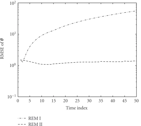
Figures 1and2present the true values of θ and an
exam-ple of estimated trajectories. As shown in both figures, two
source directions cross with each other at t = 32.
Obvi-ously, the recursive procedure designed for the most gen-eral case cannot follow fast moving sources at all. In con-trast, the estimated trajectory obtained by REM II is very
close to the true one. Figures 3and4show the root mean
square errors (RMSEs) of the DOA estimates, defined as
θt−θ2 = M
m=1(θtm−θm)2, averaged over 200 trials.
Since REM I fails to track the moving sources, the corre-sponding RMSE grows with increasing time. On the other hand, the RMSE associated with REM II decreases slightly at the beginning of the recursion and then remains almost
constant. Comparing Figures3and4, one can observe that
SNR = 20 dB has a slightly lower RMSE than SNR =
10 dB.
The second experiment involves three slowly moving
sources. The true parameter values are given by θ0 =
[30◦, 50◦, 62◦],θ1 =[0.06◦,−0.1◦, 0.05◦]. Note that the
an-gular velocityθ1is approximately 1/10 of that considered in
the previous experiment. We applied the ML method to
ob-tain the initial estimatesθ00 = [30.1◦, 50.8◦, 60.9◦]. Because
the angular velocity is very small compared to that in the
previous experiment, we takeθ01 =[0◦, 0◦, 0◦] as the initial
value forθ1. The initial estimate for REM I is given byθ00.
Both algorithms use a constant step size =0.6. Figures5
and6 present the true and estimated trajectories obtained
by REM I and REM II. Similarly to the first experiment, two
source directions cross with each other att=126. The
102
101
100
10−1
RMSE
o
f
θ
0 5 10 15 20 25 30 35 40 45 50
Time index REM I
REM II
Figure3: RMSE of θversus time for the narrowband case. SNR
=20 dB.
102
101
100
10−1
RMSE
o
f
θ
0 5 10 15 20 25 30 35 40 45 50
Time index REM I
REM II
Figure4: RMSE of θversus time for the narrowband case. SNR
=10 dB.
crossing happens. Betweent=100 andt=230, where two
source directions cross with each other, the estimated trajec-tories associated with the first two sources do not get close to
each other. Instead, they just depart in the vicinity oft=126.
For the same scenario, REM II provides a more accurate
es-timate.Figure 6shows that the crossing point causes a larger
deviation from the true trajectory. Due to a higher sensitivity to the variation of angular velocity at the crossing point, the
estimated trajectory inFigure 6is slightly worse than that in
Figure 2. Comparison of Figures7and8with Figures3and
4 shows an overall lower RMSE in this scenario. Although
REM I provides more reliable estimates than in the first ex-periment, REM II still outperforms REM I.
90 80 70 60 50 40 30 20 10 0
DO
A
(d
egr
ee
)
50 100 150 200 250 300
Time index
Figure 5: True trajectory (solid lines) and estimated trajectory (nonsolid lines) by REM I for the narrowband case. θ0 = [30◦, 50◦, 62◦],θ1=[0.06◦,−0.1◦, 0.05◦]. SNR=20 dB.
90 80 70 60 50 40 30 20 10 0
DO
A
(d
egr
ee
)
50 100 150 200 250 300
Time index
Figure 6: True trajectory (solid lines) and estimated trajectory (nonsolid lines) by REM II for the narrowband case. SNR=20 dB.
In the third experiment, three sources move slowly
with different speeds but do not cross with each other.
The true parameters are given by θ0 = [10◦, 30◦, 62◦],
θ1 = [0.08◦, 0.1◦, 0.06◦]. The initial estimates are θ00 =
[10.04◦, 30.04◦, 62.05◦],θ01 =[0◦, 0◦, 0◦]. We use a constant
step size = 0.6. Both algorithms have good tracking
abil-ity. Figures9and10show that RMSE is the lowest among
all three scenarios. REM II has a better performance than REM I. While REM II has a better performance at higher SNR, REM I seems to be less sensitive to SNRs in all three scenarios.
102
101
100
10−1
RMSE
o
f
θ
0 50 100 150 200 250 300
Time index REM I
REM II
Figure7: RMSE of θversus time for the narrowband case. SNR
=20 dB.
102
101
100
10−1
RMSE
o
f
θ
0 50 100 150 200 250 300
Time index REM I
REM II
Figure8: RMSE of θversus time for the narrowband case. SNR
=10 dB.
bins. The scenario similar to the second experiment leads to
the results presented in Figures11and12. The estimates
be-have similarly to the narrowband case. Comparison of RM-SEs shows that using more frequency bins leads to higher ac-curacy.
5.2. Comparison with LPA beamforming
We compare REM II with the LPA-based beamforming
ap-proach suggested by Katkovnik and Gershman [12]. Both
algorithms assume the motion model (16). In the first
ex-periment, the narrowband signals are generated by the
fol-lowing parameter setsθ0 = [10◦, 60◦], θ1 = [0.6◦,−1.0◦],
102
101
100
10−1
RMSE
o
f
θ
0 50 100 150 200 250
Time index REM I
REM II
Figure 9: RMSE ofθversus time for the narrowband case. SNR
=20 dB.θ0=[10◦, 30◦, 62◦],θ1=[0.08◦, 0.1◦, 0.06◦].
102
101
100
10−1
RMSE
o
f
θ
0 50 100 150 200 250
Time index REM I
REM II
Figure10: RMSE ofθversus time for the narrowband case. SNR
=10 dB.
SNR=0, 10 dB. In the second experiment, we consider
mov-ing sources with lower angular velocities θ0 = [30◦, 50◦],
θ1=[0.06◦,−0.1◦]. A sliding window of 25 snapshots is used
in the LPA beamforming. The REM II is initialized by the LPA beamforming in the first scenario and ML method in the second one. To ensure the same data length in each time
interval, we use additional (W−1) samples in the LPA
beam-forming processing.
The estimated trajectories presented in Figures13and14
are very close to the true ones. The RMSEs ofθ0andθ1
cor-responding to the first source are plotted in Figures15and
102
101
100
10−1
RMSE
o
f
θ
0 50 100 150 200 250 300
Time index REM I
REM II
Figure 11: RMSE ofθversus time for the broadband case. SNR
=20 dB.θ0=[30◦, 50◦, 62◦],θ1=[0.06◦,−0.1◦, 0.05◦]. Number of frequency bins=3.
102
101
100
10−1
RMSE
o
f
θ
0 50 100 150 200 250 300
Time index REM I
REM II
Figure 12: RMSE ofθversus time for the broadband case. SNR
=10 dB.
RMSE associated with REM II changes slowly over time.
While estimates of θ0 remain constant, the estimates ofθ1
become more accurate with increasing recursions. Also, we can observe that while LPA beamforming provides an
over-all betterθ0 estimates and better angular velocity estimates
at beginning of the recursion, REM II improvesθ1estimates
with increasing time and has less fluctuations.
Compared with the Cram´er-Rao bounds (CRBs) [23],
one realizes that an REM II is certainly not an efficient
es-timator. However, the ML approach suggested in [23], whose
estimation accuracy is close to CRB, is a batch processing and requires a complicated multidimensional search procedure.
90 80 70 60 50 40 30 20 10 0
DO
A
(d
egr
ee
)
10 20 30 40 50 60
Time index
Figure 13: True trajectory (solid lines) and estimated trajec-tory (nonsolid lines) by LPA beamforming. SNR= 10 dB.θ0 = [10◦, 60◦],θ
1=[0.6◦,−1.0◦].
90 80 70 60 50 40 30 20 10 0
DO
A
(d
egr
ee
)
10 20 30 40 50 60
Time index
Figure 14: True trajectory (solid lines) and estimated trajectory (nonsolid lines) by REM II. SNR=10 dB.
In the second experiment, REM II provides much more
accurate estimates than LPA beamforming.Figure 17shows
that LPA beamforming even fails to follow the moving
sources. We can observe inFigure 18that REM II has lower
RMSE in bothθ0andθ1estimation. Consequently, as shown
in Figures19and20the resulting DOA estimates are much
better than LPA beamforming. In both experiments, the computational time needed for LPA beamforming is about 800 times as high as that required by REM II due to the two-dimensional search procedure.
102
Figure15: (a) RMSE ofθ0corresponding to the first source versus time. (b) RMSE ofθ1versus time. SNR=10 dB.
both slowly and fast moving sources. Both procedures gener-ate accurgener-ate estimgener-ates when there is no crossing point. When two source directions coincide with each other, the steering
matrix H(θ) becomes rank deficient. The signal waveform
s(t) cannot be determined properly. Consequently the DOA
parameter cannot be estimated accurately. In this case,
regu-larization is needed [23]. Since REM II incorporates a linear
polynomial model, it has a better tracking ability than REM I when this critical situation occurs. Compared to LPA beam-forming, our method has a clear computational advantage. It provides comparable results with LPA beamforming in the fast moving sources case and outperforms LPA beamforming in the slow moving source case. In addition, REM is applica-ble to both narrowband and broadband signals.
6. CONCLUSION
We addressed the problem of tracking multiple moving sources. Two recursive procedures are proposed to estimate the time-varying DOA parameter. We applied the recursive EM algorithm to a general case in which the motion of the sources is arbitrary and a specific case in which the motion of sources is described by a linear polynomial model. Be-cause of the simple structure of the gain matrix, the suggested procedures are easy to implement. Furthermore, extension of our approaches to broadband signals is straightforward.
102
Figure16: (a) RMSE ofθ0corresponding to the first source versus time. (b) RMSE ofθ1versus time. SNR=0 dB.
Figure 17: True trajectory (solid lines) and estimated trajectory (nonsolid lines) by LPA beamforming. θ0 = [30◦, 50◦], θ1 = [0.06◦,−0.1◦]. SNR=10 dB.
102
Figure18: (a) RMSE ofθ0corresponding to the first source versus time. (b) RMSE ofθ1versus time. SNR=10 dB.
polynomial model has a better performance than the gen-eral procedure. Important issues such as step size design and convergence analysis are still under investigation.
ACKNOWLEDGMENTS
The authors thank the anonymous reviewers for their constructive comments that significantly improved the manuscript and also thank Associate Editor J. C. Chen for coordinating a speedy review.
REFERENCES
[1] J. F. B¨ohme, “Array processing,” inAdvances in Spectrum Esti-mation. Vol 2, S. Haykin, Ed., pp. 1–63, Prentice-Hall, Engle-wood Cliffs, NJ, USA, 1991.
[2] A. P. Dempster, N. Laird, and D. B. Rubin, “Maximum like-lihood from incomplete data via the EM algorithm,” J. Roy. Statist. Soc. Ser. B, vol. 39, no. 1, pp. 1–38, 1977.
[3] E. C¸ekli and H. A. C¸´yrpan, “Unconditional maximum like-lihood approach for localization of near-field sources: algo-rithm and performance analysis,”AE ¨U - International Journal of Electronics and Communications, vol. 57, no. 1, pp. 9–15, 2003.
[4] M. Feder and E. Weinstein, “Parameter estimation of super-imposed signals using the EM algorithm,”IEEE Trans. Acous-tics, Speech, and Signal Processing, vol. 36, no. 4, pp. 477–489, 1988.
Figure 19: True trajectory (solid lines) and estimated trajectory (nonsolid lines) by REM II. SNR=10 dB.
102
[5] N. Kabaoˆglu, H. A. C¸irpan, E. C¸ekli, and S. Paker, “Determin-istic maximum likelihood approach for 3-D near field source localization,” AE ¨U - International Journal of Electronics and Communications, vol. 57, no. 5, pp. 345–350, 2003.
[6] P. J. Chung and J. F. B¨ohme, “Recursive EM and SAGE algo-rithms,” inProc. IEEE Workshop on Statistical Signal Process-ing, pp. 540–542, Singapore, August 2001.
[7] D. Maiwald, Breitbandverfahren zur Signalentdeckung und – ortung mit Sensorgruppen in Seismik– und Sonaranwendungen, Doctoral thesis, Department of Electrical Engineering and In-formation Sciences, Ruhr-Universit¨at Bochum, Bochum, Ger-many, 1995.
[9] L. Frenkel and M. Feder, “Recursive expectation-maximiza-tion (EM) algorithms for time-varying parameters with ap-plications to multiple target tracking,”IEEE Trans. Signal Pro-cessing, vol. 47, no. 2, pp. 306–320, 1999.
[10] D. M. Titterington, “Recursive parameter estimation using incomplete data,”J. Roy. Statist. Soc. Ser. B, vol. 46, no. 2, pp. 257–267, 1984.
[11] A. Benveniste, M. M´etivier, and P. Priouret, Adaptive Algo-rithms and Stochastic Approximations, Source Springer Ap-plications of Mathematics Series, Springer-Verlag, New York, NY, USA, 1990.
[12] V. Katkovnik and A. B. Gershman, “A local polynomial ap-proximation based beamforming for source localization and tracking in nonstationary environments,” IEEE Signal Pro-cessing Letters, vol. 7, no. 1, pp. 3–5, 2000.
[13] P. J. Chung and J. F. B¨ohme, “Recursive EM and SAGE al-gorithms with application to DOA estimation,” to appear in IEEE Trans. Signal Processing.
[14] B. Yang, “Projection approximation subspace tracking,”IEEE Trans. Signal Processing, vol. 43, no. 1, pp. 95–107, 1995. [15] R. E. Zarnich, K. L. Bell, and H. L. Van Trees, “A unified
method for measurement and tracking of contacts from an array of sensors,” IEEE Trans. Signal Processing, vol. 49, no. 12, pp. 2950–2961, 2001.
[16] M. Wax and I. Ziskind, “Detection of the number of coherent signals by the MDL principle,”IEEE Trans. Acoustics, Speech, and Signal Processing, vol. 37, no. 8, pp. 1190–1196, 1989. [17] P. J. Chung,Fast algorithms for parameter estimation of sensor
array signals, Doctoral thesis, Department of Electrical Engi-neering and Information Sciences, Ruhr-Universit¨at Bochum, Bochum, Germany, May 2002.
[18] D. M. Titterington, A. F. Smith, and U. E. Makov, Statistical Analysis of Finite Mixture Distributions, John Wiley & Sons, New York, NY, USA, 1985.
[19] G. H. Golub and C. F. Van Loan, Matrix Computations, Johns Hopkins Studies in Mathematical Sciences, John Hop-kins University Press, Baltimore, Md, USA, 3rd edition, 1996. [20] P.-J. Chung and J. F. B¨ohme, “Recursive EM algorithm with adaptive step size,” inProc. IEEE Seventh International Sympo-sium on Signal Processing and Its Applications, vol. 2, pp. 519– 522, Paris, France, July 2003.
[21] D. R. Brillinger, Time Series: Data Analysis and Theory, Holden-Day, San Francisco, Calif, USA, 1981.
[22] J. F. B¨ohme, “Statistical array signal processing of measured sonar and seismic data,” inProc. SPIE Advanced Signal Pro-cessing Algorithms, vol. 2563 ofProceedings of SPIE, pp. 2–20, San Diego, Calif, USA, July 1995.
[23] T. Wigren and A. Eriksson, “Accuracy aspects of DOA and angular velocity estimation in sensor array processing,”IEEE Signal Processing Letters, vol. 2, no. 4, pp. 60–62, 1995.
Pei-Jung Chung received the Dr.-Ing. degree in 2002 from Ruhr-Universit¨at Bochum, Germany. From 1998 to 2002, she was with the Signal Theory Group in the Department of Electrical Engineering and Information Sciences, Ruhr-Universit¨at Bochum, Germany. From May 2002 to January 2004, she held a postdoctoral position at Carnegie Mellon University, USA. Since February 2004, she has been a
Postdoctoral Researcher at the University of Michigan, Ann Arbor, USA. Her research interests include statistical signal processing and sensor array processing.
Johann F. B¨ohmereceived the Diplom in mathematics in 1966, the Dr.-Ing. degree in 1970, and the Habilitation degree in 1977, both in computer science, from the Tech-nical University of Hannover, Germany, the University of Erlangen-Nuremberg, many, and the University of Bonn, Ger-many, respectively. From 1967 to 1974, he was with the Sonar Research Laboratory, Krupp Atlas Elektronik, Bremen, Germany.
He then joined the University of Bonn till 1978 and the FGAN in Wachtberg-Werthhoven. Since 1980, he has been a Professor of sig-nal theory in the Department of Electrical Engineering and Infor-mation Sciences, Ruhr-Universit¨at Bochum, Germany. His research interests are in the domain of statistical signal processing and its applications. He is an IEEE Fellow and recipient of the 2003 IEEE Signal Processing Society Technical Achievement Award.
Alfred O. Heroreceived the Ph.D. degree from Princeton University in 1984 in elec-trical engineering. Since 1984, he has been a Professor with the University of Michigan, Ann Arbor, Mich, USA, where he has ap-pointments in the Department of Electrical Engineering and Computer Science, the De-partment of Biomedical Engineering, and the Department of Statistics. His research interests are in the areas including