Far-ultraviolet and far-infrared bivariate luminosity function of galaxies:
Complex relation between stellar and dust emission
Tsutomu T. Takeuchi1, Akane Sakurai1, Fang-Ting Yuan1, V´eronique Buat2, and Denis Burgarella2
1Division of Particle and Astrophysical Science, Nagoya University, Furo-cho, Chikusa-ku, Nagoya 464-8602, Japan 2Laboratoire d’Astrophysique de Marseille, OAMP, Universit´e Aix-Marseille, CNRS,
38 rue Fr´ed´eric Joliot-Curie, 13388 Marseille cedex 13, France
(Received November 17, 2011; Revised June 24, 2012; Accepted June 25, 2012; Online published March 12, 2013)
Far-ultraviolet (FUV) and far-infrared (FIR) luminosity functions (LFs) of galaxies show a strong evolution fromz=0 toz=1, but the FIR LF evolves much stronger than the FUV one. The FUV is dominantly radiated from newly-formed short-lived OB stars, while the FIR is emitted by dust grains heated by the FUV radiation field. It is known that dust is always associated with star formation activity. Thus, both FUV and FIR are tightly related to the star formation in galaxies, but in a very complicated manner. In order to disentangle the relation between FUV and FIR emissions, we estimate the UV-IR bivariate LF (BLF) of galaxies withGALEXandAKARI All-Sky Survey datasets. Recently, we developed a new mathematical method to construct the BLF with given marginals and a prescribed correlation coefficient. This method makes use of a tool from mathematical statistics: the so-called “copula”. The copula enables us to construct a bivariate distribution function from given marginal distributions with a prescribed correlation and/or dependence structure. With this new formulation, and FUV and FIR univariate LFs, we analyze various FUV and FIR data withGALEX,Spitzer, andAKARI, to estimate the UV-IR BLF. The obtained BLFs naturally explain the nonlinear complicated relation between FUV and FUV-IR emission from star-forming galaxies. Though the faint-end of the BLF was not well constrained for high-zsamples, the estimated linear correlation coefficientρwas found to be very high, and is remarkably stable regarding redshifts (from 0.95 atz =0, to 0.85 atz=1.0). This implies that the evolution of the UV-IR BLF is mainly due to the different evolution of the univariate LFs, and may not be controlled by the dependence structure.
Key words:Dust, galaxies: formation, galaxies: evolution, stars: formation, infrared, ultraviolet.
1.
Introduction
Exploring the star formation history of galaxies is one of the most important topics in modern observational cosmol-ogy. In particular, the “true” absolute value of the cosmic star formation rate (hereafter SFR) has been of central im-portance to an understanding of the formation and evolution of galaxies.
However, this has been a difficult task for a long time because of dust extinction. Active star formation (SF) is al-ways accompanied by dust production through various dust grain formation processes related to the final stage of stel-lar evolution (e.g., Dwek and Scalo, 1980; Dwek, 1998; Nozawaet al., 2003; Takeuchiet al., 2005c; Asanoet al., 2013). Observationally, the SFR of galaxies are, in princi-ple, measured by the ultraviolet (UV) luminosity from mas-sive stars because of their short lifetime (∼106 yr)
com-pared with the age of galaxies or the Universe. However, since the UV photons are easily scattered and absorbed by dust grains, the SFR of galaxies is always inevitably af-fected by dust produced by their own SF activity. Since the absorbed energy is re-emitted at wavelengths of the far-infrared (FIR), we need observations both in the UV and
Copyright cThe Society of Geomagnetism and Earth, Planetary and Space Sci-ences (SGEPSS); The Seismological Society of Japan; The Volcanological Society of Japan; The Geodetic Society of Japan; The Japanese Society for Planetary Sci-ences; TERRAPUB.
doi:10.5047/eps.2012.06.008
FIR to gain an unbiased view of their SF (e.g., Buatet al., 2005; Seibert et al., 2005; Takeuchiet al., 2005a, 2010; Corteseet al., 2006; Bothwellet al., 2011; Haineset al., 2011; Haoet al., 2011).
After much effort of many researchers, the cosmic history of the SFR density is gradually converging at 0 < z < 1. This “latter half” of the cosmic SFR is characterized by the rapid decline of the total SFR, especially the decrease of the contribution of dusty IR galaxies toward z = 0: While, at z = 0, the contribution of the SFR hidden by dust is 50–60%, it becomes>90% at z = 1 (Takeuchiet al., 2005a). This difference in the decrease in SFR obtained from FUV and FIR has already been recognized in IR stud-ies (e.g., Takeuchiet al., 2001a, b). Later works have con-firmed this “dusty era of the Universe”, and revealed that the dominance of the hidden SF continues even toward higher redshifts (z∼3) (e.g., Murphyet al., 2011; Cucciatiet al., 2012).
Consequently, a natural question arises: what does the different evolution at different wavelengths represent? To address this problem, it is very important to understand how we select sample galaxies and what we see in them. Each time we find some relation between different properties, we must understand clearly which is real (physical) and which is simply due to a selection effect. Some are detected at both bands, but some are detected only at one of the ob-served wavelength and appear as upper limits at the other
wavelength. In previous studies, it was often found that various claims were inconsistent with each other, mainly because they were not based on a well-controlled sample of FUV and FIR selected galaxies. Recently, thanks to new large surveys, some attempts to explore the SFR distribu-tion of galaxies in a bivariate way have been made, through the “SFR function” (e.g., Buatet al., 2007, 2009; Bothwell et al., 2011; Haineset al., 2011). These works are based on the FUV and FIR LFs and their sum, but have not yet ad-dressed their dependence on each other. To explore further the bivariate properties of the SF in galaxies, a suitable tool is the UV-IR bivariate luminosity function (BLF).
However, constructing a BLF from two-wavelength data is not a trivial task. When we have a complete flux-limited1
multiwavelength dataset, we can estimate a univariate lu-minosity function (LF) at each band, but what we want to know isthe dependence structurebetween luminosities at different bands. Mathematically, this problem is rephrased as follows: can we (re)construct a multivariate probabil-ity densprobabil-ity function (PDF) satisfying prescribed marginals? Although there is an infinite number of degrees of freedom to choose the original PDF, if we can model the dependence between variables, we can construct such a bivariate PDF. A statistical tool for this problem is the so-called “copula” (see Section 2 for the definition).
The copula has been extensively used in financial engi-neering, for instance, but until recently there have been very few applications to astrophysical problems (e.g., Benabed et al., 2009; Koen, 2009; Satoet al., 2010, 2011; Scher-reret al., 2010). Takeuchi (2010) introduced the copula to the estimation problem of a BLF. In this work, we apply a copula-based BLF estimation to the UV-IR two-wavelength dataset fromz=0 toz=1, using data fromIRAS,AKARI2,
Spitzer3, andGALEX4.
The layout of this paper is as follows: We define a copula, in particular the Gaussian copula, and formulate the copula-based BLF in Section 2. We then describe our UV and IR data in Section 3. In Section 4, we first formulate the likelihood function for the BLF estimation. Then, we show the results, and discuss the possible interpretation of the evolution of the UV-IR BLF. Section 5 is devoted to the summary.
Throughout the paper, we will assume M0 = 0.3, 0 =0.7 and H0 =70 km s−1Mpc−1. The luminosities
are defined asνLν and expressed in solar units assuming L=3.83×1033erg s−1.
2.
The Bivariate Luminosity Function Based on
the Copula
1Or any other observational condition.2URL: http://www.ir.isas.ac.jp/ASTRO-F/index-e.html. 3URL: http://www.spitzer.caltech.edu/.
4URL: http://www.galex.caltech.edu/.
ate DF. We note that all bivariate DFs have this form and we can safely apply this method to any kind of bivariate DF estimation problem (Takeuchi, 2010). In various applica-tions, we usually know the marginal DFs (or equivalently, the PDFs) from the data. The problem then reduces to a statistical estimation of a set of parameters to determine the shape of the copulaC(u1,u2). In the form of the PDF,
Since the choice of copula is literally unlimited, we have to introduce a guidance principle. In many data analyses in physics, the most familiar measure of dependence might be the linear correlation coefficientρ. Mathematically speak-ing,ρdepends not only on the dependence of two variables but also the marginal distributions, which is not an ideal property as a dependence measure. Even so, a copula hav-ing an explicit dependence onρ would be convenient. In this work, we use a copula with this property: the Gaussian copula.
One of the natural candidates withρ may be a copula related to a bivariate Gaussian DF (for other possibilities, see Takeuchi, 2010). The Gaussian copula has an explicit dependence on a linear correlation coefficient by its con-struction. Let
The density ofCG,cG, is obtained as
andIstands for the identity matrix.
2.3 Construction of the UV-IR BLF
In this work, we define the luminosity at a certain wave-length band byL≡νLν(νis the corresponding frequency). Then the LF is defined as the number density of galax-ies whose luminosity lgalax-ies between the logarithmic interval [logL,logL+d logL]:
φ(1)(L)≡ dn
d logL , (10)
where we denote logx ≡ log10x and lnx ≡ logex. For
mathematical simplicity, we define the LF as being normal-ized, i.e.,
φ(1)(L)d logL =1. (11)
Hence, this corresponds to a PDF. We also define a cumu-lative LF as
(1)(L)≡ logL
logLmin
φ(1)(L)d logL, (12)
whereLminis the minimum luminosity of galaxies
consid-ered. This corresponds to the DF. If we denote the univari-ate LFs asφ1(1)(L1)andφ2(1)(L2), then the BLFφ(2)(L1,L2)
For the Gaussian copula, the BLF is obtained as
φ(2)(L
For the UV LF, we adopt the Schechter function (Schechter, 1976):
For the IR, we use the analytic form for the LF proposed by Saunderset al.(1990):
We use the re-normalized version of Eqs. (17) and (16) so that they can be regarded as PDFs, as mentioned above.
2.4 Selection effects: another benefit of the copula BLF
Another benefit of the copula is that it is easy to incor-porate observational selection effects which always exist in any kind of astronomical data. In a bi(multi)variate analy-sis, there are two categories of observational selection ef-fects:
1) Truncation
We do not know if a source would exist below a detec-tion limit.
2) Censoring
We know there is a source, but we have only an upper (sometimes lower) limit for a certain observable.
As mentioned above, we have to deal with both of these se-lection effects carefully to construct a BLF from the data at the same time. It is terribly difficult to incorporate these effects by heuristic methods: particularly for nonparamet-ric methods (Takeuchi, 2012, in preparation). In contrast, since we have an analytic form for the BLF, the treatment of upper limits is much more straightforward (Takeuchi, 2010). We show how it is treated in the likelihood function in Section 4.
3.
Data
3.1 UV-IR data construction
We have constructed a dataset of galaxies selected at FUV and FIR byGALEX andIRASfor z = 0. At higher redshifts,GALEXandSpitzerdata are used forz=0.7 and EIS (ESO Imaging Survey) and Spitzerforz=1.0 in the Chandra Deep Field South (CDFS). We explain the details of each sample in the following.
In the Local Universe, we used the sample compiled by Buatet al.(2007). This sample was constructed based on theIRASall-sky survey and the GALEX All-Sky Imaging Survey (AIS). This dataset consists of UV- and IR-selected samples. The UV-selection was made by theGALEXFUV (λ = 1530 ˚A) band with FUV < 17 mag (hereafter, all magnitudes are presented in AB mag). This corresponds to the luminosity lower limit of LFUV > 108 L.
Red-shift information was taken from HyperLEDA (Paturelet al., 2003) and NED. The IR-selection is based on theIRAS PSCz (Saunderset al., 2000). The detection limit of the PSCz is S60 > 0.6 Jy. Redshifts of all PSCz galaxies
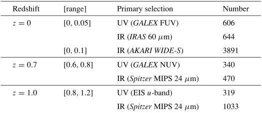
Table 1. Sample description.
Redshift [range] Primary selection Number
z=0 [0,0.05] UV (GALEXFUV) 606
IR (IRAS60μm) 644
[0,0.1] IR (AKARI WIDE-S) 3891
z=0.7 [0.6,0.8] UV (GALEXNUV) 340 IR (SpitzerMIPS 24μm) 470
z=1.0 [0.8,1.2] UV (EISu-band) 319 IR (SpitzerMIPS 24μm) 1033
We also constructed a new, much larger sample of IR-selected galaxies byAKARIFIS All-Sky Survey. We started from theAKARIFIS bright source catalog (BSC) v.1 from theAKARI all sky survey (Yamamura et al., 2010). This sample is selected at theWIDE-Sband (λ = 90 μm) of theAKARIFIS (Kawadaet al., 2007). The detection limit is S90 > 0.2 Jy. We first selected AKARI sources in the
SDSS footprints to have the same solid angle with a (forth-coming) corresponding UV-selected sample we are prepar-ing with GALEX-SDSS.5 Then, to have a secure sample of galaxies with redshift data, we made a cross-match of AKARIsources with the ImperialIRAS-FSC Redshift Cata-logue (IIFSCz), a redshift catalog recently published (Wang and Rowan-Robinson, 2009), with a search radius of 36 arc-sec. Since about 90% of galaxies in the IIFSCz have spec-troscopic, or photometric, redshifts at S60 > 0.36 Jy, the
depth of the sample is defined by this matching. This deter-mines the redshift range of this dataset to be approximately z < 0.1. We measured the FUV and NUV flux densities with the same procedure as theIRAS-GALEXsample. The detection limits at FUV and NUV of this sample are 19.9 mag and 20.8 mag (Morrisseyet al., 2007). A correspond-ing UV-selected sample is under construction: hence, we only have an IR-selected sample. The number of galaxies is 3,891. For more information on this sample and the proper-ties of galaxies, see Sakuraiet al.(2013).
At higher-z, our samples are selected in the CDFS. GALEXobserved this field at FUV and NUV (2300 ˚A) as a part of its deep imaging survey. We restricted the field to the subfield observed bySpitzer/MIPS, as a part of the GOODS key program (Elbazet al., 2007), to have the corresponding IR data. The area of the region is 0.068 deg2. A precise
description of our high-zsamples is presented in Buatet al. (2009) and Burgarellaet al.(2006).
At z = 0.7, the NUV-band corresponds to the rest-frame FUV of the sample galaxies. We thus constructed the sample based on NUV-selection. Redshifts were taken from the COMBO-17 survey (Wolfet al., 2004), and we have defined thez = 0.7 sample as those with redshifts of 0.6 < z < 0.8. Data reduction and redshift associa-tion are explained in Burgarellaet al.(2006). We truncated the sample at NUV = 25.3 mag so that more than 90 % of the GALEX sources are identified in COMBO-17 with
5This step is not a mandatory in this study, but we are planning to make an extension of this analysis with the UV-selected data, and this step will make the analysis easier with respect to the treatment of survey areas when the UV-selected data will be ready.
R < 24 mag. We set the MIPS 24 μm upper limit as 0.025 mJy for undetected sources. For the IR-selected sam-ple, we based on the GOODSSpitzer/MIPS 24μm sample and matched theGALEXand COMBO-17 sources. The sizes of the UV- and IR-selected samples are 340 and 470, respectively.
In contrast toz=0.7, since NUV ofGALEXcorresponds to 1155 ˚A in the rest frame of galaxies at z = 1.0, we cannot use NUV as the primary selection band as the rest-frame FUV. Instead, we selected galaxies in theU-band from the EIS survey (Arnoutset al., 2001) that covers the CDFS/GOODS field. We then cross-matched theU-band sources with the COMBO-17 sample to obtain redshifts. For thez =1 sample, the range of redshifts is 0.8 < z < 1.2. We set the limit at U = 24.3 mag to avoid source confusion. The IR flux densities were taken fromSpitzer MIPS 24μm data, and the same upper limit as thez=0.7 sample is taken for non-detections. Again, the IR-selected sample was constructed from the GOODS and matched the GALEXand COMBO-17 sources, as thez = 0.7 sample. The sizes of thez = 1.0 UV and IR-selected samples are 319 and 1033, respectively.
The characteristics of these samples are summarized in Table 1.
3.2 Far-UV and total IR luminosities
We are interested in the SF activity of galaxies and its evolution. Hence, luminosities of galaxies representative of SF activity would be ideal. As for the directly-visible SF, obviously the UV emission is appropriate for this pur-pose. We define the FUV luminosity of galaxies,LFUV, as
LFUV≡νLν@FUV. Forz=0 galaxies, FUV corresponds
to 1530 ˚A. At higher redshifts, as we have explained,LFUV
is calculated from the NUV flux density atz=0.7 and the U-band flux density atz=1.0, respectively.
In contrast, at IR, the luminosity related to the SF activ-ity is the one integrated over a whole range of IR wave-lengths (λ = 8–1000 μm), LTIR, where the subscript TIR
stands for the total IR. For the Local IRAS-GALEX sam-ple, it is quite straightforward to defineLTIRsince theIRAS
galaxies are selected at 60 μm. We adopted the formula LTIR = 2.5νLν@60μm. This rough approximation is, in
fact, justified by the spectral energy distributions (SEDs) of galaxies withISO 160 μm observations (Takeuchi et al., 2006).
2005b, 2010),
However, since deep FIR data of higher-zgalaxies are not easily available to date, we should rely on the data taken by SpitzerMIPS 24μm. We use the conversion formulae from MIR luminosity toLTIR:
logLTIR[L]=1.23+0.972 logL15[L], (20)
logLTIR[L]=2.27+0.707 logL12[L]
+0.0140(logL12[L])2, (21)
which are an updated version of the formulae proposed by Takeuchiet al.(2005b) and also used by Buatet al.(2009). Here,L15andL12are luminositiesνLν@15μm and 12μm,
i.e., 24/(1+z)atz =0.7 and 1.0, respectively. The esti-matedLTIR depends slightly on which kind of conversion
formula is used; but for our current purpose, it does not af-fect our conclusion and we do not discuss this extensively here. An intercomparison of the MIR-TIR conversion for-mulae can be found in Buatet al.(2009).
This situation will be greatly improved withHerschel6
data. We will leave this to our future work with theHerschel H-ATLAS (Eales et al., 2010) and GAMA (Galaxy And Mass Assembly: Driveret al., 2011) data (Takeuchiet al., 2012, in preparation).
4.
Results and Discussion
4.1 FUV and TIR univariate LFs
In order to estimate the UV-IR BLF, first we have to ex-amine our setting for the FUV and TIR univariate LFs. The IRAS-GALEX sample, the validity of the Local univariate LFs are already proved (see figure 3 of Buatet al., 2007). Hence, we can safely use the analytic formulae of FUV and TIR LFs atz=0 (Eqs. (16) and (17)).
We use the Schechter parameters presented by Wyderet al.(2005) forGALEXFUV:(α1,L∗1, φ∗1)=(1.21,1.81×
al., 2003) obtained from theIRASPSCzgalaxies (Saunders et al., 2000), and multipliedL∗1with 2.5 to convert the 60-μm LF to the TIR LF.
For higher redshifts, ideally we should estimate the uni-variate FUV and TIR LFs simultaneously with the BLF es-timation. This is, however, quite difficult with our current samples, because of the limited number of galaxies. We used, instead, the LF parameters atz=0.7 and 1.0 obtained by previous studies on univariate LFs and modeled the FUV and TIR univariate LFs at these redshifts and examined their validity with nonparametric LFs estimated from the data. We use the parameters compiled by Takeuchiet al.(2005a).
6URL: http://herschel.esac.esa.int/.
Parameters of the evolution of the TIR LF are obtained by approximating the evolution in the form
φ(1) Le Floc’het al.(2005) assumed a power-law form for the evolution functions as
f(z)=(1+z)Q, g(z)=(1+z)P, (23)
and obtained P = 0.7 and Q = 3.2, with α remaining constant. The Schechter parameters atz=0.7 and 1.0 for the FUV LF are directly estimated by Arnoutset al.(2005) and we adopt their values (see table 1 of Takeuchi et al., 2005a).
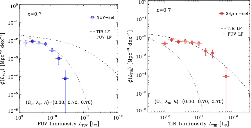
Then, we estimated the FUV and TIR LFs using the step-wise maximum likelihood method and the variant of theC− method from our CDFS multiwavelength data (for the esti-mation method, see, e.g., Takeuchiet al., 2000; Johnston, 2011, and references therein). The obtained univariate LFs atz =0.7 and 1.0 are presented in Figs. 1 and 2. We also show the analytic model LFs in these figures. We note that a well-known large density enhancement locates in the CDFS atz =0.7 (e.g., Salimbeniet al., 2009), and thus we have renormalized the LFs to remove the effect of the overden-sity. In the following analysis, we normalize the univariate LFs according to Eq. (11) so that we can treat the univari-ate LFs as PDFs; hence, this does not affect the following analysis at all.
Because of the small sample size, the LF shape does not perfectly agree with the supposed functional forms, but the nonparametric LFs are acceptably similar to the analytic functions both for the FUV and TIR at each redshift. We stress that the analytic functions arenotthe fit to the data, but estimated from other studies. This implies that the es-timated evolutionary parameters of the LFs work generally well. Thus, we can use the higher-zunivariate LFs as the marginal PDFs for the estimation of the UV-IR BLFs.
4.2 Copula likelihood for the BLF estimation
By using the estimated univariate FUV and TIR LFs as given marginals, we can estimate only one parameter, the linear correlationρby maximizing the likelihood func-tion. The structure of a set of two-band selected data is
(Lik
or IR) stands for the upper limit flag: jband = 0: detection
and jband = −1: upper limit. Another index,k, is the
in-dicator of the selected band, i.e., k = 1 means a sample galaxy is selected at UV andk= −1 means it is selected at IR. The likelihood function is as follows:
Fig. 1. The FUV and TIR LFs at z = 0.7 (left and right panel, respectively). Open squares are nonparametric LFs estimated from our CDFS multiwavelength data withGALEXNUV- andSpitzerMIPS 24μm selections. Dotted lines represent the FUV LFs at this redshift bin taken from Arnoutset al.(2005). Dashed lines depict the TIR LFs derived from the evolutionary parameters atz=0.7 given by Le Floc’het al.(2005). Because of a well-known large density enhancement at this redshift, we renormalized the LF to remove the effect of the overdensity.
Fig. 2. The FUV and TIR LFs atz=1.0. Symbols are the same as in Fig. 1, but FUV samples are selected at theU-band.
where pdetLik
FUV,L ik
TIR
is the probability for the ikth
galaxy to be detected at both bands and to have luminosities Lik
FUVandL
ik
TIR,
pdet
Lik
FUV,L ik
TIR
≡ φ
(2)Lik
FUV,L ik
TIR;ρ ∞
Llim FUV(zik)
∞
Llim TIR(zik)
φ(2)L
FUV,LTIR;ρ
dLTIRdLFUV
,
(25)
pUL:UV
Lik
FUV,L ik
TIR
is the probability for theikth galaxy
to be detected at the IR band and have a luminosity Lik
TIR,
but not detected at the UV band and only an upper limit Lik
FUV,jk is available,
pUL:UV
Lik
FUV,L ik
TIR
≡
LikFUV,jk
0
φ(2)L
FUV,L ik
TIR
dLFUV
∞
0 ∞
Llim TIR(zik)
φ(2)L
FUV,LTIR;ρ
dLTIRdLFUV
,
(26)
and pUL:IR
Lik
FUV,L ik
TIR
is the probability for the ikth
luminos-ityLik
FUV, but not detected at the IR band and only an upper
limitLik
TIR,jk is available,
pUL:IR
Lik
FUV,L ik
TIR
≡
LikTIR,jk
0
φ(2)Lik
FUV,LTIR
dLTIR
∞
Llim FUV(zik)
∞
0
φ(2)L
FUV,LTIR;ρ
dLTIRdLFUV
.
(27)
The denominator in Eq. (25) is introduced to take into ac-count the truncation in the data by observational flux se-lection limits at both bands (e.g., Sandage et al., 1979; Johnston, 2011). We should also note that it often happens that the same galaxies are included in both the UV- and IR-selected sample. In such a case, we should count the same galaxies only once to avoid double counting of them. Prac-tically, such galaxies are included in any of the samples, because they are detected at both bands and are symmetric between UV- and IR-selections.
In the estimation procedure, we estimated the univariate LFs and their evolutions first, and then used these parame-ters to estimate the BLF and its evolution. One might won-der if this compromising method would introduce some bias in the estimation. Since we fix the form of the maximum likelihood estimator Eq. (24), this two-step estimation, in-stead of simultaneous estimation, does not bias the result, especially the dependence structure between UV and IR, unless the assumed univariate LF shape would be signifi-cantly different from the real one. We have already seen that the stepwise maximum likelihood estimation gave non-parametric LFs which agree reasonably with the assumed Schechter, or Saunders, function. Then, we can safely rely on the result for further discussion.
However, we should note that the two-step estimation gives conditional errors of the parameters only for each step, not the marginal ones. Then, the errors for each of the parameters are significantly underestimated. If we want to discuss the error values more precisely, we need a larger dataset and must use the simultaneous estimation method. This will be done in future work.
4.3 The BLF and its evolution
Using the Gaussian copula, we can now estimate the BLF. The visible and hidden SFRs should be directly re-flected to this function. Dust is produced by SF activity, but also destroyed by SN blast waves as a result of the SF. Many physical processes are related to the evolution of the dust amount. Thus, first of all, we should describe statisti-cally how it evolved, as stated in Introduction.
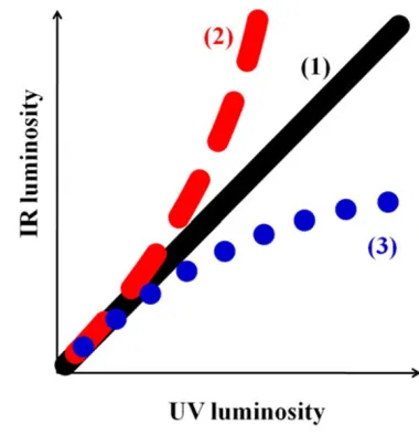
First, we summarize how to interpret the UV-IR BLF shown schematically in Fig. 3. First, we see the case that the ridge of the BLF is straight and diagonal (see (1) in Fig. 3). This means that the energy from SF is emitted equally at UV and IR with any SF activity. If the relation is diagonal, but has an offset horizontally or vertically, this suggests that a constant fraction of energy is absorbed by dust and re-emitted. Second, if the ridge is curved upward, it means that the more active the SF in a galaxy is, the more luminous at the IR (dusty SF: (2) in Fig. 3). Third, if the
Fig. 3. Schematic BLF. (1) Diagonal: The energy from SF is emitted equally at UV and IR with any SF activity. (2) Upward: The more active the SF in a galaxy is, the more luminous at the IR (dusty SF). (3) Downward: The more active the SF is, the more luminous at the UV (transparent SF).
ridge is bent downward, the more active the SF is, the more luminous at UV (‘transparent’ SF: (3) in Fig. 3).
Now, we show the estimated BLFs in Figs. 4–7. In the Local Universe, the BLF is quite well constrained. The estimated correlation coefficientρis very high:ρ=0.95± 0.04 forIRAS-GALEXandρ =0.95±0.006 for AKARI-GALEX datasets. The apparent scatter of the LFUV–LTIR
is found to be due to the nonlinear shape of the ridge of the BLF. This bent shape of the BLF was implied by preceding studies (Martinet al., 2005), and we have been able to quantify this feature. The copula BLF naturally reproduced it. For theAKARI-GALEXsample, only the IR-selected sample is available at this moment. This, however, does not bias the BLF estimation since the information from censored data points are incorporated properly in Eq. (24). This can be directly tested, for example, by using only one of the UV and IR-selected data for the z = 0 BLF estimation with the IRAS-GALEX dataset. Both one-band estimations with UV- and IR-selected data yieldρ=0.95± 0.07. Obviously the error becomes larger because of fewer data, but the estimate itself remain unchanged.
At higher redshifts (z =0.7–1.0), the linear correlation remains tight (ρ 0.91±0.06 atz=0.7 andρ 0.86± 0.05 atz=1.0), even though it is difficult to constrain the low-luminosity end from the data in this analysis (Spitzer-GALEXin the CDFS). The distribution of upper limits in Figs. 6 and 7 looks different from that in Fig. 4. Since we have restricted the redshifts of galaxies in these samples, the redshift restriction gives approximately constant luminosity limits both at FUV and FIR. This gives the “L-shaped” distribution of upper limits seen in these figures.
Fig. 4. The BLF of galaxies fromIRASandGALEXatz=0. Contours are the analytic model constructed by a Gaussian copula and univariate FUV and TIR LFs. Open squares represent the UV-selected sample fromGALEX, while open triangles are the IR-selected ones fromIRAS. Squares and triangles with arrows mean that they are the upper limits at FUV and FIR, respectively.
Fig. 5. The same as Fig. 4 but fromAKARIandGALEX. Open trian-gles represent the IR-selected samples fromAKARI. Since there is no UV-selected sample in this figure, we only show the IR-selected ones.
evolution of the univariate LFs, and may not be controlled by the evolution of the dependence structure.
Forthcoming better data in the future will improve vari-ous aspects of the BLF estimation. First,Herschel, ALMA, andSPICA7will provide us with direct estimations ofL
TIR
of galaxies, especially at high redshifts, since they will de-tect these galaxies at longer wavelengths than 24μm. This allows us to avoid a possible bias of the estimated LTIR
caused by the 24-μm-based extrapolation of the SED.
7URL: http://www.ir.isas.jaxa.jp/SPICA/SPICA HP/index English.html.
Fig. 6. The same as Fig. 4 but fromSpitzerandGALEXatz = 0.7. Symbols are essentially the same as in Fig. 4, but IR-selected samples are fromSpitzer/MIPS.
Fig. 7. The same as Fig. 4 but fromSpitzerandGALEXatz=1.0. Again symbols are essentially the same as in Fig. 4, but IR-selected samples are fromSpitzer/MIPS.
enable any conclusions on the faint-end dependence struc-ture of the BLF, but, again,Herschel, ALMA, andSPICA data, together with ground-based optical orJWSTdata, will enable us to examine which copula would be appropriate to describe the BLF, and to constrain the evolution of the BLF along the whole history of galaxy evolution in the Uni-verse.
5.
Conclusion
To understand the visible and hidden SF history in the Universe, it is crucial to analyze multiwavelength data in a unified manner. The copula is an ideal tool to combine two marginal univariate LF to construct a bivariate LFs. It is straightforward to extend this method to multivariate DFs.
1) The Gaussian copula LF is sensitive to the linear cor-relation parameterρ.
2) Even so, ρ in the copula LF is remarkably stable re-garding redshifts (from 0.95 at z = 0 to 0.85 at z=1.0).
3) This implies the evolution of the UV-IR BLF is mainly due to the different evolution of the univariate LFs, and may not be controlled by the dependence structure. 4) The nonlinear structure of the BLF is naturally
repro-duced by the Gaussian copula.
The data fromHerschel, ALMA, andSPICAdata will im-prove the estimates drastically, and we expect to specify the full evolution of the UV-IR BLF in the Universe. We stress that the copula will be a useful tool for any other kind of bi-(multi-) variate statistical analysis.
Acknowledgments. This work is based on observations with
AKARI, a JAXA project with the participation of ESA. This re-search has made use of the NASA/IPAC Extragalactic Database (NED) which is operated by the Jet Propulsion Laboratory, Cal-ifornia Institute of Technology, under contract with the National Aeronautics and Space Administration. TTT has been supported by the Program for Improvement of Research Environment for Young Researchers from Special Coordination Funds for Promot-ing Science and Technology, and the Grant-in-Aid for the Scien-tific Research Fund (20740105, 23340046, 24111707) commis-sioned by the MEXT. TTT, AS, and FTY have been partially sup-ported from the Grant-in-Aid for the Global COE Program “Quest for Fundamental Principles in the Universe: from Particles to the Solar System and the Cosmos” from the Ministry of Education, Culture, Sports, Science and Technology (MEXT) of Japan.
References
Arnouts, S.et al., ESO imaging survey. Deep public survey: Multi-color optical data for the Chandra Deep Field South,Astron. Astrophys.,379, 740–754, 2001.
Arnouts, S.et al., TheGALEXVIMOS-VLT Deep Survey Measurement of the Evolution of the 1500 ˚A Luminosity Function,Astrophys. J.,619, L43–L46, 2005.
Asano, R. S., T. T. Takeuchi, H. Hirashita, and A. K. Inoue, Dust formation history of galaxies: A critical role of metallicity for the dust mass growth by accreting materials in the interstellar medium,Earth Planets Space, 65, this issue, 213–222, 2013.
Benabed, K., J.-F. Cardoso, S. Prunet, and E. Hivon, TEASING: a fast and accurate approximation for the low multipole likelihood of the cosmic microwave background temperature,Mon. Not. R. Astron. Soc.,400, 219–227, 2009.
Bothwell, M. S., R. C. Kennicutt, B. D. Johnson, Y. Wu, J. C. Lee, D. Dale, C. Engelbracht, D. Calzetti, and E. Skillman, The star formation rate distribution function of the local Universe,Mon. Not. R. Astron. Soc.,415, 1815–1826, 2011.
Buat, V.et al., Dust attenuation in the nearby universe: A comparison be-tween galaxies selected in the ultraviolet and in the far-infrared, Astro-phys. J.,619, L51–L54, 2005.
Buat, V., T. T. Takeuchi, J. Iglesias-P´aramoet al., The local universe as seen in the far-infrared and far-ultraviolet: A global point of view of the local recent star formation,Astrophys. J. Suppl. Ser.,469, 19–25, 2007. Buat, V., T. T. Takeuchi, D. Burgarella, E. Giovannoli, and K. L. Murata, The infrared emission of ultraviolet-selected galaxies fromz = 0 to
z=1,Astron. Astrophys.,507, 693–704, 2009.
Burgarella, D.et al., Ultraviolet-to-far infrared properties of Lyman break galaxies and luminous infrared galaxies atz∼ 1,Astron. Astrophys., 450, 69–76, 2006.
Cortese, L., A. Boselli, V. Buat, G. Gavazzi, S. Boissier, A. Gil de Paz, M. Seibert, B. F. Madore, and D. C. Martin, UV dust attenuation in normal star-forming galaxies. I. Estimating theLTIR/LFUVratio,Astrophys. J., 637, 242–254, 2006.
Cucciati, O.et al., The star formation rate density and dust attenuation evolution over 12 Gyr with the VVDS surveys,Astron. Astrophys.,539, A31, 2012.
Driver, S. P.et al., Galaxy and Mass Assembly (GAMA): survey diag-nostics and core data release,Mon. Not. R. Astron. Soc.,413, 971–995, 2011.
Dwek, E., The evolution of the elemental abundances in the gas and dust phases of the galaxy,Astrophys. J.,501, 643, 1998.
Dwek, E. and J. M. Scalo, The evolution of refractory interstellar grains in the solar neighborhood,Astrophys. J.,239, 193–211, 1980.
Eales, S.et al., TheHerschelATLAS,Publ. Astron. Soc. Pac.,122, 499– 515, 2010.
Elbaz, D.et al., The reversal of the star formation-density relation in the distant universe,Astron. Astrophys.,468, 33–48, 2007.
Haines, C. P., G. Busarello, P. Merluzzi, R. J. Smith, S. Raychaudhury, A. Mercurio, and G. P. Smith, ACCESS—II. A complete census of star for-mation in the Shapley supercluster—UV and IR luminosity functions,
Mon. Not. R. Astron. Soc.,412, 127–144, 2011.
Hao, C.-N., R. C. Kennicutt, B. D. Johnson, D. Calzetti, D. A. Dale, and J. Moustakas, Dust-corrected star formation rates of galaxies. II. Combinations of ultraviolet and infrared tracers,Astrophys. J.,741, 124 (22pp), 2011.
Iglesias-P´aramo, J.et al., Star formation in the nearby universe: The ultra-violet and infrared points of view,Astrophys. J. Suppl. Ser.,164, 38–51, 2006.
Johnston, R., Shedding light on the galaxy luminosity function,Astron. Astrophys. Rev.,19, 41, 2011.
Kawada, M.et al., The Far-Infrared Surveyor (FIS) forAKARI,Publ. Astron. Soc. Jpn.,59, 389–400, 2007.
Koen, C., Confidence intervals for the correlation between the gamma-ray burst peak energy and the associated supernova peak brightness,Mon. Not. R. Astron. Soc.,393, 1370–1376, 2009.
Le Floc’h, E.et al., Infrared luminosity functions from the Chandra Deep Field-South: TheSpitzerview on the history of dusty star formation at 0≤z≤1,Astrophys. J.,632, 169–190, 2005.
Martin, D. C.et al., The star formation rate function of the local universe,
Astrophys. J.,619, L59–L62, 2005.
Morrissey, P.et al., The calibration and data products ofGALEX,Astron. Astrophys.,173, 682–697, 2007.
Murphy, E. J., R.-R. Chary, M. Dickinson, A. Pope, and D. T. Frayer, An accounting of the dust-obscured star formation and accretion histories over the last∼11 billion years,Astrophys. J.,732, 126 (17pp), 2011. Nozawa, T., T. Kozasa, H. Umeda, K. Maeda, and K. Nomoto, Dust in
the early universe: Dust formation in the ejecta of population III super-novae,Astrophys. J.,598, 785–803, 2003.
Paturel, G., C. Petit, P. Prugniel, G. Theureau, J. Rousseau, M. Brouty, P. Dubois, and L. Cambr´esy, HYPERLEDA. I. Identification and designa-tion of galaxies,Astron. Astrophys.,412, 45–55, 2003.
Sakurai, A., T. T. Takeuchi, F.-T. Yuan, V. Buat, and D. Burgarella, Star formation and dust extinction properties of local galaxies as seen from AKARI and GALEX,Earth Planets Space,65, this issue, 203–211, 2013.
Salimbeni, S.et al., A comprehensive study of large-scale structures in the GOODS-SOUTH field up toz∼2.5,Astron. Astrophys.,501, 865–877, 2009.
Sato, M., K. Ichiki, and T. T. Takeuchi, Precise estimation of cosmological parameters using a more accurate likelihood function,Phys. Rev. Lett., 105, 251301, 2010.
Sato, M., K. Ichiki, and T. T. Takeuchi, Copula cosmology: Constructing a likelihood function,Phys. Rev. D,83, 023501, 2011.
Saunders, W., M. Rowan-Robinson, A. Lawrence, G. Efstathiou, N. Kaiser, R. S. Ellis, and C. S. Frenk, The 60-micron and far-infrared lu-minosity functions ofIRASgalaxies,Mon. Not. R. Astron. Soc.,242, 318–337, 1990.
Saunders, W.et al., The PSCz catalogue,Mon. Not. R. Astron. Soc.,317, 55–63, 2000.
Schechter, P., An analytic expression for the luminosity function for galax-ies, Astrophys. J.,203, 297–306, 1976.
Scherrer, R. J., A. A. Berlind, Q. Mao, and C. K. McBride, From finance to cosmology: The copula of large-scale structure,Astrophys. J.,708, L9–L13, 2010.
Seibert, M.et al., Testing the empirical relation between ultraviolet color and attenuation of galaxies,Astrophys. J.,619, L55–L58, 2005. Takeuchi, T. T., Constructing a bivariate distribution function with given
marginals and correlation: application to the galaxy luminosity function,
Mon. Not. R. Astron. Soc.,406, 1830–1840, 2010.
Takeuchi, T. T., K. Yoshikawa, and T. T. Ishii, Tests of statistical methods for estimating galaxy luminosity function and applications to the Hubble deep field,Astrophys. J. Suppl. Ser.,129, 1–31, 2000.
Takeuchi, T. T., T. T. Ishii, H. Hirashita, K. Yoshikawa, H. Matsuhara, K. Kawara, and H. Okuda, Exploring galaxy evolution from infrared number counts and cosmic infrared background,Publ. Astron. Soc. Jpn., 53, 37–52, 2001a.
Takeuchi, T. T., R. Kawabe, K. Kohno, K. Nakanishi, T. T. Ishii, H. Hi-rashita, and K. Yoshikawa, Impact of future submillimeter and millime-ter large facilities on the studies of galaxy formation and evolution,
Publ. Astron. Soc. Pac.,113, 586–606, 2001b.
Takeuchi, T. T., K. Yoshikawa, and T. T. Ishii, The luminosity function of
IRASpoint source catalog redshift survey galaxies,Astrophys. J.,587,
L89–L92, 2003.
Takeuchi, T. T., V. Buat, and D. Burgarella, The evolution of the ultraviolet and infrared luminosity densities in the universe at 0<z<1,Astron. Astrophys.,440, L17–L20, 2005a.
Takeuchi, T. T., V. Buat, J. Iglesias-P´aramo, A. Boselli, and D. Burgarella, Mid-infrared luminosity as an indicator of the total infrared luminosity of galaxies,Astron. Astrophys.,432, 423–429, 2005b.
Takeuchi, T. T., T. T. Ishii, T. Nozawa, T. Kozasa, and H. Hirashita, A model for the infrared dust emission from forming galaxies,Mon. Not. R. Astron. Soc.,362, 592–608, 2005c.
Takeuchi, T. T., T. T. Ishii, H. Dole, M. Dennefeld, G. Lagache, and J.-L. Puget, The ISO 170 μm luminosity function of galaxies,Astron. Astrophys.,448, 525–534, 2006.
Takeuchi, T. T., V. Buat, S. Heinis, E. Giovannoli, F.-T. Yuan, J. Iglesias-P´aramo, K. L. Murata, and D. Burgarella, Star formation and dust ex-tinction properties of local galaxies from theAKARI-GALEXall-sky sur-veys. First results from the most secure multiband sample from the far-ultraviolet to the far-infrared,Astron. Astrophys.,514, A4, 2010. Wang, L. and M. Rowan-Robinson, The imperialIRAS-FSC redshift
cata-logue,Mon. Not. R. Astron. Soc.,398, 109–118, 2009.
Wolf, C.et al., A catalogue of the Chandra Deep Field South with multi-colour classification and photometric redshifts from COMBO-17, As-tron. Astrophys.,421, 913–936, 2004.
Wyder, T. K.et al., The ultraviolet galaxy luminosity function in the local universe fromGALEXdata,Astrophys. J.,619, L15–L18, 2005. Yamamura, I., S. Makiuti, N. Ikeda, Y. Fukuda, S. Oyabu, T. Koga, and
G. J. White,AKARI/FIS all-sky survey bright source catalogue version 1.0 release note, ISAS/JAXA, 2010.