! " # # "$ % %#
& ''' (
Maximum Entropy
Functions of Discrete Random Fuzzy Variables and
Genetic Algorithm
Lianlong Gao*
College of Science,
Guilin University of Technology
Guilin, P.R.China
Liang Lin
College of Science,
Guilin University of Technology
Guilin, P.R.China
Abstract: Due to deficiency of information, the membership functions and probability distribution of a random fuzzy variable cannot be ob-tained explicitly. It is a challenging work to find an appropriate membership function and an appropriate probability distribution when certain
partial information about a random fuzzy variable is given, such as expected value or moments. This paper solves such problems for the
maximum entropy of discrete random fuzzy variables with certain constraints. A genetic algorithm is designed to solve the general maximum
entropy model for discrete random fuzzy variables, which is illustrated by some numerical experiments.
Keywords:Random fuzzy variables; Chance measure; Entropy; Genetic algorithm
I INTRODUCTION
We usually meet many uncertain phenomena because
“uncertainty is absolute and certainty is relative” in the real
world. In these uncertain events, fuzziness and randomness
are two basic types of uncertainty. Probability theory is a
branch of mathematics for studying the behavior of random
phenomena. The study of probability theory was started by
Pascal and Fermat (1654), and an axiomatic foundation of
probability theory was given by Kolmogoroff (1933) in his
Foundations of Probability Theory. Credibility theory is a branch of mathematics for studying the behavior of fuzzy
phenomena. The study of credibility theory was started by
Liu and Liu (2002), and an axiomatic foundation of
credi-bility theory was given by Liu (2004) in his Uncertainty Theory. Sometimes, fuzziness and randomness simulta-neously appear in a system. In order to describe this
phe-nomena, a random fuzzy variable was proposed by Liu [12]
as a fuzzy element taking “random variable” values. In
ad-dition, a hybrid variable was introduced by Liu [13] as a
tool to describe the quantities with fuzziness and
random-ness. Fuzzy random variable and random fuzzy variable are
instances of hybrid variable. In order to measure hybrid
events, a concept of chance measure was introduced by Li
and Liu [14].
Entropy is use to provide a quantitative measurement
of the degree of uncertainty, which has widely been applied
in transportation [19]&[20], risk analysis [22], signal
processing [21] and economics [25]. Since the Shannon
entropy of random variables was proposed by Shannon [6],
Jaynes [15] provided the maximum entropy principle of
random variables when some constraints were given. Fuzzy
entropy was first initialized by Zadeh [7] to quantify the
fuzziness, who defined the entropy of a fuzzy event as a
weighted Shannon entropy. Up to now, fuzzy entropy has
been studied by many researchers such as De Luca and
Termini [4], Kaufmann [5], Yager [17], Kosko [16], Pal and
Pal [10], Bhandari and Pal [1], Pal and Bezdek [11].
How-ever, those definitions of entropy characterize the
uncer-tainty resulting primarily from the linguistic vagueness
ra-ther than resulting from information deficiency, and
va-nishes when the fuzzy variable is an equipossible one. In
order to measure the uncertainty of fuzzy variables, Liu [9]
suggested that an entropy of fuzzy variables should meet at
least three basic requirements: (i) minimum; (ii) maximum;
(iii) universality. In order to meet those requirements, Li
and Liu [8] provided a new definition of fuzzy entropy to
characterize the uncertainty resulting from information
de-ficiency which is caused by the impossibility to predict the
specified value that a fuzzy variable takes and provided the
maximum entropy principle of fuzzy variables. In order to
measure the uncertainty of hybrid variables, Li X, and Liu
given some constraints, for example, expected value and
variance, there are usually multiple compatible membership
functions and probability distributions. Which membership
functions and probability distributions shall we take?
Be-cause fuzziness and randomness simultaneously appear in a
system, we can not get the maximum entropy of hybrid
variables through Euler-Lagrange equation. For fuzzy
va-riables, Li and Liu [2] gave an analytical method to find the
maximum entropy membership function of continuous
fuzzy variables and Gao and You [3] gave an analytical
method to find the maximum entropy membership function
of discrete fuzzy variables. On the basis of their work we
promote their ideas to solve the problem for maximum
en-tropy functions of discrete random fuzzy variables in this
paper.
The organization of our work is as follows: In section
2, some basic concepts and results on random fuzzy
va-riables are reviewed. In section 3, we introduce some
con-straints. In sections 4 and 5, an effective genetic algorithm
is introduced to solve general maximum entropy models for
discrete random fuzzy variables and some computational
experiments are given in illustration of it. Finally, the
con-clusion is given in the last section.
II. PRELIMINARIES
Let
ξ
be a fuzzy variable with the membershipfunc-tion
µ
( )
x
which satisfies the normalization condition,i.e.,
sup
xµ
( )
x
=
1
. In the setting of credibility theory, the credibility measure for fuzzy event{
ξ
∈
B
}
deducedfrom
µ
( )
x
is given by{
}
1
( )
( )
Cr
sup
1 sup
2
x B x BcB
x
x
ξ
µ
µ
∈ ∈
∈
=
+ −
(2.1)
Where
B
is any subset of the real numbersR
, andB
cis the complement of set
B
. Conversely, for a fuzzyvaria-ble
ξ
, its membership function can be derived from thecredibility measure by
( )
x
(
2Cr
{
x
}
)
1,
x
R
µ
=
ξ
=
∧
∈
(2.2)Definition 2.1 (X.Li, B.Liu [23]) A random fuzzy variable
is a function from a credibility space
(
Θ
, , Cr
P
)
to the set of random variables defined on a probability space(
Ω
, , Pr
A
)
.In the following, we give some examples of random
fuzzy variables.
Example 2.1 (Uniformly distributed random fuzzy variable)
A random fuzzy variable
ξ
is said to be uniform if foreach
θ
,ξ θ
( )
is a uniformly distributed randomva-riables, i.e.,
ξ θ
( )
~
U X
( ) ( )
θ
,
Y
θ
, withX
andY
are fuzzy variables defined on the spaceΘ
such thatX
≤
Y
.Example 2.2 (Normally distributed random fuzzy variable)
A random fuzzy variable
ξ
is said to be normal if foreach
θ
,ξ θ
( )
is a normally distributed random variable,i.e.,
ξ θ
( )
∈
N X
(
( ) ( )
θ
,
Y
θ
)
, withX
andY
are fuzzy variables defined on the spaceΘ
such thatY
>
0
. A normally distributed random fuzzy variable is usuallydenoted as
ξ
∈
N X Y
(
,
)
, and the fuzziness of randomfuzzy variable
ξ
is said to be characterized by fuzzyvec-tor
(
X Y
,
)
.Example 2.3 (Exponentially distributed random fuzzy
va-riable) A random fuzzy variable
ξ
is said to beexponen-tial if for each
θ
,ξ θ
( )
is an exponentially distributedrandom variable whose density function is defined as
( )
( )
( )
(
( )
)
0,
0
exp
,
0
t
f
t
X
X
t
t
ξ θ
θ
θ
<
=
−
≥
(2.3)
Θ
. An exponentially distributed random fuzzy variables is often denoted byξ
~ exp
( )
X
, and the fuzziness ofran-dom fuzzy variable
ξ
is said to be characterized by fuzzyvariable
X
.Generally, let
ξ
be a random fuzzy variable. Thefuzziness of
ξ
is said to be characterized by fuzzyvaria-ble
X
, if for eachθ
∈ Θ
, the distribution of random va-riableξ θ
( )
is determined by the parameterX
( )
θ
.Definition 2.2 (Li and Liu [18]) Let
(
Θ
, , Cr
P
) (
× Ω
, , Pr
A
)
be a chance space. Then a chance measure of an eventΛ
is defined as{ }
{ }
{
( )
}
(
)
{ }
{
( )
}
(
)
{ }
{
( )
}
(
)
{ }
{
( )
}
(
)
sup Cr
Pr
,
sup Cr
Pr
0.5
Ch
1 sup Cr
Pr
,
sup Cr
Pr
0.5
c
if
if
θ θ θ θθ
θ
θ
θ
θ
θ
θ
θ
∈Θ ∈Θ ∈Θ ∈Θ∧
Λ
∧
Λ
<
Λ =
−
∧
Λ
∧
Λ
≥
(2.4)
In fact, chance measure may be defined in different
ways. For example, we may employ the following chance
measure,
{ }
1
sup
(
( )
Pr
{
( )
}
)
1 sup
(
( )
Pr
{
( )
}
)
2
c
Ch
θ θ
µ θ
θ
µ θ
θ
∈Θ ∈Θ
Λ =
×
Λ
+ −
×
Λ
(2.5)
Where
µ θ
( )
=
(
2
Cr
{ }
θ
)
∧
1
.Theorem 2.1 (Li X, Liu B [24]) Let
(
Θ
, , Cr
P
) (
× Ω
, , Pr
A
)
be a chance space andCh
a chance measure. Then for any eventΛ
, we have{ }
{
( )
}
(
)
(
{ }
{
( )
}
)
sup Cr
Pr
sup Cr
Pr
c0.5
θ θ
θ
θ
θ
θ
∈Θ ∈Θ
∧
Λ
∨
∧
Λ
≥
(2.6)
{ }
{
( )
}
(
)
(
{ }
{
( )
}
)
sup Cr
Pr
sup Cr
Pr
c1
θ θ
θ
θ
θ
θ
∈Θ ∈Θ
∧
Λ
+
∧
Λ
≤
(2.7)
Proof: It follows from the basic properties of probability and credibility that
{ }
{
( )
}
(
)
(
{ }
{
( )
}
)
sup Cr
Pr
sup Cr
Pr
cθ θ
θ
θ
θ
θ
∈Θ ∈Θ
∧
Λ
∨
∧
Λ
{ }
(
{
( )
}
{
( )
}
)
(
)
sup Cr
Pr
Pr
cθ
θ
θ
θ
∈Θ
≥
∧
Λ
∨
Λ
{ }
sup Cr
0.5
0.5
θ
θ
∈Θ≥
∧
=
and{ }
{
( )
}
(
)
(
{ }
{
( )
}
)
sup Cr
Pr
sup Cr
Pr
cθ θ
θ
θ
θ
θ
∈Θ ∈Θ
∧
Λ
+
∧
Λ
{ }
{
( )
}
{ }
{
( )
}
(
)
1 2
1 1 2 2
,
sup Cr
Pr
Cr
Pr
cθ θ
θ
θ
θ
θ
∈Θ
=
∧
Λ
+
∧
Λ
{ }
{ }
(
)
(
{
( )
}
{
( )
}
)
1 2
1 2
sup Cr
Cr
sup Pr
Pr
cθ θ θ
θ
θ
θ
θ
≠ ∈Θ
≤
+
∨
Λ
+
Λ
≤ ∨ =
1 1 1
.Example 2.4: Let
η η
1,
2,
,
η
m be random variables, and letu u
1,
2,
,
u
m be nonnegative numbers with1 2 m
1
u
∨
u
∨
∨
u
=
. Then1 1
2 2
with membership degree
with membership degree
with membership degree
m m
u
u
u
η
η
ξ
η
=
(2.8)is clearly a random fuzzy variable. If
η η
1,
2,
,
η
m have probability density functionsφ φ
1,
2,
,
φ
m, respectively, then for any Borel setB
of real numbers,{
}
( )
( )
( )
( )
1 1
1 1
max , if max 0.5
2 2
Ch
1 max , if max 0.5
2 c 2
i i
i i
B B
i m i m
i i
i i
B B
i m i m
u u
x dx x dx
B
u u
x dx x dx
φ φ
ξ
φ φ
≤ ≤ ≤ ≤
≤ ≤ ≤ ≤
∧ ∧ <
∈ =
− ∧ ∧ ≥
(2.9)
variable. Then the expected value of
ξ
is defined by
[ ]
0Ch
{
}
0Ch
{
}
E
ξ
+∞ξ
r dr
ξ
r dr
−∞
=
≥
−
≤
(2.10)
provided that at least one of the two integrals is finite.
In fact, the expected value
E
[ ]
ξ
ofξ
may bede-fined by
[ ]
0{
|
( )
}
0{
|
( )
}
E
ξ
+∞Cr
θ
E
ξ θ
r dr
Cr
θ
E
ξ θ
r dr
−∞
=
∈Θ
≥
−
∈Θ
≤
(2.11)
provided that at least one of the two integrals is finite,
where
E
ξ θ
( )
is the expected value of randomvaria-ble
ξ θ
( )
.According to the Li and Liu [23] we get a new
defini-tion of entropy of random fuzzy variable
ξ
, denoted by[ ]
H
ξ
.Definition 2.4 Suppose that
ξ
is a discrete random fuzzyvariable taking values in
{
x x
1,
2,
}
. Then its entropy isdefined by
[ ]
(
{
}
)
1
Ch
ii
H
ξ
S
ξ
x
∞
=
=
=
.(2.12)
where
S t
( )
= −
t
ln
t
−
(
1
−
t
) (
ln 1
−
t
)
. If there existssome index
k
such thatCh
{
ξ
=
x
k}
=
1
, and 0 other-wise, then its entropyH
[ ]
ξ
=
0
. Suppose thatξ
is a simple random fuzzy variable taking values in{
x x
1,
2,
,
x
n}
. IfCh
{
ξ
=
x
i}
=
0.5
for all1, 2,
,
i
=
n
, then its entropyH
[ ]
ξ
=
n
ln 2
. Supposethat
ξ
is a discrete random fuzzy variable taking values in{
x x
1,
2,
}
. ThenH
[ ]
ξ
≥
0
and equality holds if andonly if
ξ
is essentially a deterministic / crisp number.III. MOMENT CONSTRAINTS
In this section, we consider discrete random fuzzy
va-riables. Let
ξ
be a discrete random fuzzy variable takingvalues in
{
x x
1,
2,
,
x
n}
(in this paper we always as-sume thatx
1<
x
2<
<
x
n) with membership degrees{
u u
1,
2,
,
u
n}
and probability{
p p
1,
2,
,
p
n}
,re-spectively, where
u
1∨
u
2∨
∨
u
n=
1.
Then theex-pected value of
ξ
can be written as (without loss ofgene-rality, suppose
x
k−1< ≤
0
x
k).[ ]
{
}
{
}
{
}
{
}
1 1 1
1 0
0
1 2
Ch Ch Ch Ch
k i i
i i k
n k
x x x
x x x
i k i
Eξ ξ r dr ξ r dr ξ r dr ξ r dr
− − − − = + = = ≥ + ≥ − ≤ − ≤
{
}
{
}
(
)
(
{
}
{
}
)
1 1Ch Ch Ch Ch
k n
i i i i i i
i i k
x x x x x x
ξ
ξ
ξ
ξ
−
= =
= ≤ − < ⋅ + ≥ − > ⋅
1 1 1 1 1 1 1
max max max max
2 2 2 2 2
max 0.5&max 0.5
2 2
1
1 max max
2 2 2
n
j j j j
j j j j i
j i j i i j n i j n
i
j j
j j
j i i j n
n
j j
j j
i j n j i
i
u u u u
p p p p x
u u
if p p
u u
p p
≤ ≤ ≤ < ≤ ≤ < ≤
=
≤ ≤ ≤ ≤
< ≤ ≤ < =
∧ − ∧ + ∧ − ∧ ⋅
∧ < ∧ <
= − ∧ − ∧
1
1
Similarly, five forms can be intro
1 max max
2 2
0.5&max 0.5&max 0.5
2 2 2
duced
j j
j j i
j i i j n
j j
i
j j
j i i j n
u u
p p x
u u
u
if pi p p
≤ < < ≤
≤ < < ≤
+ − ∧ − ∧ ⋅
∧ ≥ ∧ < ∧ <
1 n i i i
x
ω
==
(3.1)It is easy to verify that all
ω
i≥
0
and1
1
n i
{
}
1
max
max
0.5,
1, 2,
,
2
2
j j
j j
j i i j n
u
u
p
p
i
n
≤ ≤
∧
∨
< ≤∧
≥
∈
, then
1
1
n i i=
ω
=
.Furthermore,
E
(
ξ
−
e
)
2 is called the variance ofξ
and
E
ξ
n the nth moment ofξ
. If the random fuzzy variableξ
reduces to a fuzzy variable, i.e., for any{
1, 2,
,
}
i
∈
n
,p
i≡
1
, then the expected value reduces to the following form
[ ]
(
1 1)
1
1
max
max
max
max
2
n
j j j j i
j i j i i j n i j n i
E
ξ
u
u
u
u
x
≤ ≤ ≤ < ≤ ≤ < ≤
=
=
−
+
−
⋅
(3.2)
Which is just the expected value of discrete fuzzy variable
ξ
. Thus, the expected value of discrete random fuzzyva-riable is a natural extension of discrete fuzzy vava-riable. Let
ξ
be a nonnegative discrete random fuzzy variable takingvalues in
{
x x
1,
2,
,
x
n}
with membership degrees{
u u
1,
2,
,
u
n}
and probability{
p p
1,
2,
,
p
n}
,re-spectively., where , and
k
a positive number. Then the k-th moment{
}
1 0
k k
E
ξ
=
k
+∞r
−Ch
ξ
≥
r dr
{
}
1
.
n
k i i i
k
Ch
ξ
x
x
=
=
≥
1
1 1
max
if max
0.5
2
2
1 max
if max
0.5
2
2
n
j k j
j i j
i j n i j n
i n
j k j
j i j
j i i j n
i
u
u
k
p
x
p
u
u
k
p
x
p
≤ ≤ ≤ ≤
=
≤ < ≤ ≤
=
∧
⋅
∧
<
=
−
∧
⋅
∧
≥
(3.3)
If the random fuzzy variable
ξ
reduces to a fuzzy variable,i.e., for any
i
∈
{
1, 2,
,
n
}
,p
i≡
1
, then the k-th mo-ment reduces to the following form{
}
1 0
k k
E
ξ
=
k
+∞r
−Cr
ξ
≥
r dr
{
}
1
.
n
k i i i
k
Cr
ξ
x
x
=
=
≥
(
1)
1
1
max
1 max
2
n
k
j j i
i j n j i i
k
u
u
x
≤ ≤ ≤ <
=
=
+ −
⋅
(3.4)
Which is just the k-th moment of discrete fuzzy variable
ξ
.If
k
=
1
, which is just the expected value of discrete ran-dom fuzzy variableξ
.IV. GENETIC ALGORITHM FOR GENERAL MAX-IMUM ENTROPY MODEL
Genetic algorithm is a stochastic search method for
global optimization problems based on the mechanics of
natural selection and natural genetics. Genetic algorithm
has demonstrated enormous success in providing good
so-lutions to many complex optimization problems. In this
section, we will design an effective genetic algorithms
inte-grated with random fuzzy simulation for solving the
maxi-mum entropy model for discrete random fuzzy variables.
Let
ξ
be a discrete random fuzzy variable takingvalues in
{
x x
1,
2,
,
x
n}
with membership degrees{
u u
1,
2,
,
u
n}
and probability{
p p
1,
2,
,
p
n}
,re-spectively. We have the natural relation
0
≤
u
i≤
1
,0
≤
p
i≤
1
andmax
1≤ ≤i nu
i=
1
. By using maximum entropy principle, we have the following{
}
(
)
{
}
1
1
1
max
subject to
,
0
1,
1, 2,
, .
0
1,
1, 2,
,
1,
1, 2,
,
1
n
i i
n i i i
i i i n
i i
S Ch
x
x
e
u
i
n
p
i
n
u
i
n
ξ
ω
ω
==
=
=
≤
≤
≤
=
≤
≤
=
=
∈
=
(4.1)
Where
ω
i from (3.1),( )
ln
(
1
) (
ln 1
)
S t
= −
t
t
−
−
t
−
t
,{
}
1
0.5
2
2
1 max
0.5
2
2
i i
i i
i
j i
j i
j n j i
u
u
p
p
Ch
x
u
u
p
p
ξ
≤ ≤ ≠
∧
∧
<
=
=
−
∧
∧
≥
.
In general, the expected value constraint can be
re-placed by other moment constraints. For the search spaces
of the maximum entropy model (4.1) are particularly
irre-gular, genetic algorithm has succeeded in providing good
solutions to complex moment conditions.
As an illustration, the following steps show how the
genetic algorithm works.
Step 1: Initialize pop-size feasible chromosomes
{
1,
2,
,
}
t t t
t n
U
=
u u
u
andP
t=
{
p p
1t,
2t,
,
p
nt}
for1, 2,
,
t
=
pop-size from(
0,1
) (
×
0,1
)
×
×
(
0,1
)
, inwhich the maximum t
,
1, 2,
,
i
u i
=
n
for eacht
is set to be 1.Step 2: Calculate the expected values for all
chromo-somes
U
t andP
t,t
=
1, 2,
,
pop-size, respectively. If the expected values do not satisfy the constraints, werege-nerate a chromosome to replace the original one until it is feasible.
Step 3: Calculate the entropy of each random fuzzy variable which is represented by each chromosome. The
entropy denoted by
H U
(
t∧
P
t)
, is to assign a probabil-ity of reproduction to each chromosomeU
t andP
t so that its likelihood of being selected is proportional to itsentropy relative to the other chromosomes in the population.
That is, the chromosomes with larger entropy will have
more chance to produce offspring by using roulette wheel
selection.
Step 4: Select the chromosomes for a new population
by spinning the roulette wheel according to the value of the
entropy of all chromosomes.
Step 5: Renew the chromosomes by crossover
opera-tions with a predetermined parameters
P
c, which is called the probability of crossover. In order to determine thepar-ents for crossover operation, let us do the following process
repeatedly from
t
=
1
to pop-size: generating a random numberr
from the interval[ ]
0,1
, the chromosomeU
tand
P
t is selected as a parent ifr
<
P
c. We denote theselected parents by
U U
1t,
2t,
U
3t,
and
1
,
2,
3,
t t t
P P P
and divide them into the following pairs:(
1,
2) (
,
3,
4) (
,
5,
6)
,
t t t t t t
U U
U
U
U
U
(
1,
2) (
,
3,
4) (
,
5,
6)
,
t t t t t t
P P
P P
P P
Let us illustrate the crossover operator on each pair by
(
1,
2)
t t
U U
and(
P P
1t,
2t)
. At first, we generate a randomnumber
c
from the open interval(
0,1
)
. Then thecros-sover operator on
U
1t andU
2t,P
1t andP
2t will pro-duce two childrenX
andY
,X
′
andY
′
as follows:(
)
(
)
1
1
2,
1
1 2t t t t
X
= ⋅
c U
+
−
c U
⋅
Y
=
−
c U
⋅
+ ⋅
c U
(
)
(
)
1
1
2,
1
1 2t t t t
X
′
= ⋅
c P
+
−
c
⋅
P Y
′
=
−
c
⋅
P
+ ⋅
c P
set the maximum component of each child to be 1. Then we
check if the children satisfy the constraints. If both children
are feasible, then we replace the parents with them. If not,
we keep the feasible child if it exists, and keep the other
parent still.
Step 6: Update the chromosomes by mutation
opera-tions with a predetermined probability of mutation
P
m. In a similar manner to the process of selecting parents forcrossover operation, we repeat the following steps from
1
t
=
to pop-size: generating a random numberr
from the interval[ ]
0,1
, the chromosomeU
t andP
t is se-lected as a parent ifr
<
P
m. For each selected parent,de-noted by
{
1t,
2t,
,
t}
t n
U
=
u u
u
and{
1,
2,
,
}
t t t
t n
P
=
p p
p
, we mutate it in the following way.For each selected parent, we randomly select one
u
it andt i
p
of this chromosome and regenerate their values. Thenset the maximum
u
it to be 1 and check the feasibility of it.Step 7: Repeat Step 3 to Step 6 for
N
times, whereN
is a sufficiently large integer.Step 8: Report the best chromosome
U
t andP
t as the optimal solution.V. NUMERICAL EXAMPLES
In order to illustrate the effectiveness of the proposed
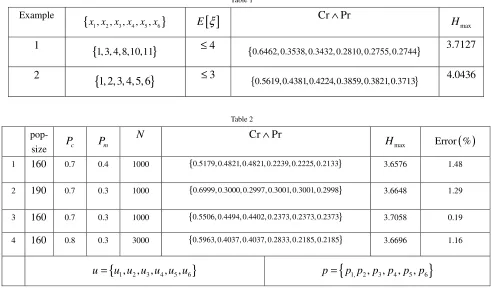
genetic algorithm, let us consider Example 1 in Table 1 (
ξ
is a discrete random fuzzy variable taking values in
{
1, 3, 4,8,10,11
}
withp
=
{
1,1,1,1,1,1
}
and expectedvalue
E
[ ]
ξ
satisfyingE
[ ]
ξ
≤
4
) for the comparison of the algorithm with respect to different parameters (Gaoand You [3]). We compare the solutions when different
pa-rametric values of
P
c,P
m,pop
−
size
andN
are taken in the genetic algorithm. The results are shown in Figand the errors shown in Table 2 are calculated by the
[image:7.612.60.551.433.722.2]for-mula: (actual value-optimal value)/optimal value
×
100%
.Table 1
Example
{
x x x x x x1, 2, 3, 4, 5, 6}
E
[ ]
ξ
Cr
∧
Pr
max
H
1
{
1, 3, 4, 8,10,11}
≤
4
{
0.6462, 0.3538, 0.3432, 0.2810, 0.2755, 0.2744}
3.7127
2
{
1, 2, 3, 4, 5, 6
}
≤
3
{
0.5619, 0.4381, 0.4224, 0.3859, 0.3821, 0.3713}
4.0436
Table 2
pop-
size
P
cP
mN
Cr
∧
Pr
max
H
Error %( )
1 160 0.7 0.4 1000 {0.5179, 0.4821, 0.4821, 0.2239, 0.2225, 0.2133} 3.6576 1.48
2 190 0.7 0.3 1000 {0.6999, 0.3000, 0.2997, 0.3001, 0.3001, 0.2998} 3.6648 1.29
3 160 0.7 0.3 1000 {0.5506, 0.4494, 0.4402, 0.2373, 0.2373, 0.2373} 3.7058 0.19
4 160 0.8 0.3 3000 {0.5963, 0.4037, 0.4037, 0.2833, 0.2185, 0.2185} 3.6696 1.16
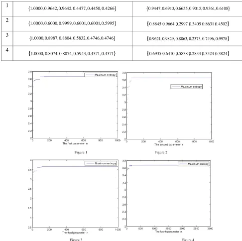
{
1,
2,
3,
4,
5,
6}
1
{
1.0000, 0.9642, 0.9642, 0.4477, 0.4450, 0.4266}
{
0.9447, 0.6913, 0.6655, 0.9015, 0.9361, 0.6108}
2
{
1.0000, 0.6000, 0.9999, 0.6001, 0.6001, 0.5995}
{
0.8845 0.9664 0.2997 0.3405 0.8631 0.4502}
3
{
1.0000, 0.8987, 0.8804, 0.5832, 0.4746, 0.4746}
{
0.9621, 0.9829, 0.8863, 0.2373, 0.7496, 0.9978}
4
{
1.0000, 0.8074, 0.8074, 0.5943, 0.4371, 0.4371}
{
0.6935 0.6410 0.5838 0.2833 0.3524 0.3824}
[image:8.612.59.545.56.540.2]
Figure 1 Figure 2
Figure 3 Figure 4
It follows from Table that the error does not exceed
3%
, which shows that the proposed algorithm is effective to solve the above model.VI. CONCLUSIONS
In this paper, we promote the idea of Gao and You [3]
to solve this problem for maximum Entropy functions of
discrete random fuzzy variables and design a genetic
algo-rithm to solve this problem. Along with the improvement of
uncertainty theory, we can use this method to solve many
uncertain events such as toward fuzzy. In the future work,
we will continue focus on this area.
VII. ACKNOWLEDGMENT
This work was partially supported by the Guangxi
Na-tional Science Foundation of China (Gui No. 0832261)
VIII. REFERENCES
[1] Bhandari D, and Pal NR, Some new information measures
of fuzzy sets, Information Sciences, Vol.67, 209-228,
1993.
va-riables, International Journal of Uncertainty Fuzziness
&Knowledge-Based Systems15(Supplement 2) (2007)
43-52.
[3] X. Gao, C. You, Maximum entropy membership functions
for discrete fuzzy variables, Information Sciences 179
(2009) 2353-2361.
[4] De Luca A, and Termini S, A definition of
non-probabilistic entropy in the setting of fuzzy sets
theory, Information and Control, Vol.20, 301-312,1972.
[5] Kaufmann A, Introduction to the Theory of Fuzzy
Arith-metic: Theory and Applications, Van Nostrand Reinhold,
New York, 1985.
[6] Shannon C., The Mathematical Theory of Communication,
The University of Illinois Press, Urbana, 1949.
[7] Zadeh L, Probability measures of fuzzy events, Journal of
Mathematical Analysis and Applications, vol.23,421-427,
1968.
[8] Li P, and Liu B, Entropy of credibility distributions for
fuzzy variables, IEEE Transactions on Fuzzy Systems,
Vol.16, No.1, 123-129, 2008
[9] Liu B, A survey of entropy of fuzzy variables, Journal of
Uncertain Systems, Vol.1, No.1, 4-13, 2007.
[10] Pal NR, and Pal SK, Object background segmentation
using a new definition of entropy, IEE Proc. E, Vol.136,
284-295, 1989.
[11] Pal NR, and Bezdek JC, Measuring fuzzy uncertainty,
IEEE Transactions on Fuzzy Systems, Vol.2, 107-118,
1994.
[12] Liu B, Theory and Practice of Uncertain Programming,
Physica-Verlag,Heidel-berg,2002.
[13] Liu B, A survey of credibility theory, Fuzzy Optimization
and Decision Making,Vol.5, No.4, 387-408,2006.
[14] Li X, Liu B, Chance measure for hybrid events with
fuz-ziness and randomness, Soft Computing , Vol.13, No.2,
105-115, 2009.
[15] Jaynes ET, Information theory and statistical mechanics,
Physical Reviews, Vol.106, No.4, 620-630, 1957.
[16] Kosko B, Fuzzy entropy and conditioning, Information
Sciences, Vol.40, 165-174, 1986.
[17] Yager RR, On measures of fuzziness and negation, Part I:
Membership in the unit interval, International Journal of
General Systems, Vol.5,221-229, 1979.
[18] B.Liu, Theory and Practice of Uncertain Programming,
Physica-Verlag, Heidelberg(2002).
[19] B.Samanta, T.K.Roy, Multi-objective entropy
transporta-tion model with trapezoidal fuzzy number penalties,
sources and destination, Journal of Transportation
Engi-neering 131 (6) (2005) 419-428.
[20] S. Islam, T.K. Roy, A new fuzzy multi-objective
pro-gramming: Entropy based geometric programming and its
application of transportation problems, European Journal
of Operational Research 173 (2006) 387-404.
[21] M.M. Stecker, The entropy of a constrained signal: A
maximum entropy approach with applications , Signal
Processing, Volume 88, Issue 3,March 2008, 639-669.
[22] L.Feng,W.Hong, On the principle of maximum entropy
and the risk analysis of disaster loss, Applied
Mathemat-ical Modelling, Volume 33, Issue7, July 2009,
2934-2938.
[23] Y.Liu, B.Liu, Expected value operator of random fuzzy
variable and random fuzzy expected value models,
Inter-national Journal of Uncertainty,Fuzziness and
Know-ledge-Based Systems, Vol.11, No.2 (2003), 195-215.
[24] X.Li, B.Liu, Chance measure for hybrid events with
fuz-ziness and randomness, Soft Comput (2009) 13:105-115.
[25] X.Wu, Calculation of maximum entropy densities with
application to income distribution, Journal of