Scholarship@Western
Scholarship@Western
Electronic Thesis and Dissertation Repository
May 2012
Fuzzy Differential Evolution Algorithm
Fuzzy Differential Evolution Algorithm
Dejan VuceticThe University of Western Ontario
Supervisor
Dr. Slobodan Simonovic
The University of Western Ontario
Graduate Program in Civil and Environmental Engineering
A thesis submitted in partial fulfillment of the requirements for the degree in Master of Engineering Science
© Dejan Vucetic 2012
Follow this and additional works at: https://ir.lib.uwo.ca/etd
Part of the Civil and Environmental Engineering Commons, Electrical and Computer Engineering Commons, and the Operations Research, Systems Engineering and Industrial Engineering Commons
Recommended Citation Recommended Citation
Vucetic, Dejan, "Fuzzy Differential Evolution Algorithm" (2012). Electronic Thesis and Dissertation Repository. 503.
https://ir.lib.uwo.ca/etd/503
This Dissertation/Thesis is brought to you for free and open access by Scholarship@Western. It has been accepted for inclusion in Electronic Thesis and Dissertation Repository by an authorized administrator of
(Spine title: Fuzzy Differential Evolution Algorithm with Application in Water Resource Systems)
(Thesis format: Monograph)
by
Dejan Vucetic
Graduate Program in Civil and Environmental Engineering
A thesis submitted in partial fulfillment of the requirements for the degree of
Master of Engineering Science
The School of Graduate and Postdoctoral Studies The University of Western Ontario
London, Ontario, Canada
ii
School of Graduate and Postdoctoral Studies CERTIFICATE OF EXAMINATION
Supervisor
______________________________ Dr. Slobodan Simonovic
Supervisory Committee
______________________________
______________________________
Examiners
______________________________ Dr. Jagath Samarabandu
______________________________ Dr. Jason Gerhard
______________________________ Dr. Ashraf Nassef
______________________________
The thesis by
Dejan Vucetic
entitled:
Fuzzy Differential Evolution Algorithm
is accepted in partial fulfillment of the requirements for the degree of Master of Engineering Science
______________________ _______________________________
iii
Abstract
The Differential Evolution (DE) algorithm is a powerful search technique for solving global optimization problems over continuous space. The search initialization for this algorithm does not adequately capture vague preliminary knowledge from the problem domain. This thesis proposes a novel Fuzzy Differential Evolution (FDE) algorithm, as an alternative approach, where the vague information of the search space can be represented and used to deliver a more efficient search. The proposed FDE algorithm utilizes fuzzy set theory concepts to modify the traditional DE algorithm search initialization and mutation
components. FDE, alongside other key DE features, is implemented in a convenient decision support system software package. Four benchmark functions are used to demonstrate
performance of the new FDE and its practical utility. Additionally, the application of the algorithm is illustrated through a water management case study problem. The new algorithm shows faster convergence for most of the benchmark functions.
Keywords
iv
Acknowledgments
I am very grateful for my supervisor, Dr. S.P. Simonovic for giving me the opportunity to do research in this exciting field. He has generously offered his time and followed my work with keen interest from its inception. He has shared his infinite knowledge and provided
motivation to increase my own. I consider it a great privilege and honor to call myself one of his students.
v
Table of Contents
CERTIFICATE OF EXAMINATION ... ii
Abstract ... iii
Acknowledgments... iv
Table of Contents ... v
List of Tables ... viii
List of Figures ... x
List of Appendices ... xii
Chapter 1 ... 1
1 Introduction ... 1
1.1 Organization of the Thesis ... 7
Chapter 2 ... 8
2 Methodology ... 8
2.1 Differential Evolution Algorithm ... 8
2.1.1 DE Population Initialization ... 9
2.1.2 Mutation ... 11
2.1.3 Crossover ... 12
2.1.4 Selection ... 13
2.1.5 Termination ... 13
2.1.6 Illustrative Example of Classic DE Algorithm ... 14
2.2 Selected Differential Evolution Algorithm Variants ... 17
2.2.1 DE/best/1/bin ... 17
vi
2.3.1 Fuzzy Adaptive Differential Evolution ... 21
2.4 Constraints ... 25
2.4.1 Search Space Constraint ... 26
2.4.2 Feasible Space Constraint ... 27
2.5 Fuzzy Differential Evolution Algorithm ... 30
2.5.1 Initialization ... 30
2.5.2 Mutation ... 34
2.5.3 Illustrative Example of FDE Algorithm ... 36
Chapter 3 ... 42
3.1 Decision Support System Software Package ... 42
3.2 Differential Evolution Optimizer Overview ... 42
3.2.1 Algorithm Inputs ... 44
3.2.2 Optimization Inputs ... 48
3.2.3 Optimization Results ... 50
3.3 Illustrative Example ... 52
Chapter 4 ... 56
4.1 Application ... 56
4.2 Benchmark Functions ... 56
4.2.1 Benchmark Function Results and Discussions ... 62
4.3 Case Study ... 68
4.3.1 Study Area Background ... 68
4.3.2 Problem Definition... 71
4.3.3 Mathematical Formulation ... 71
4.3.4 Algorithm and Optimization Inputs ... 75
vii
5.1 Summary ... 84
5.2 Recommendations for Future Work... 85
References ... 87
Appendices ... 92
viii
List of Tables
Table 2.1. Population vector matrix for each generation ... 11
Table 2.2. An illustrative example ... 15
Table 2.3. Calculation of the weighted difference vector for the illustrative example ... 15
Table 2.4. Calculation of the mutated vector for the illustrative example ... 16
Table 2.5. Generation of the trial vector for the illustrative example ... 16
Table 2.6. New population for the next generation in the illustrative example ... 17
Table 2.7. Membership Functions ... 23
Table 2.8. The Fuzzy Rules ... 24
Table 2.9. An illustrative example ... 38
Table 2.10. Calculation of the weighted difference vector for the illustrative example ... 38
Table 2.11. Calculation of the mutated vector for the illustrative example ... 39
Table 2.12. Interval to single value mutated vector calculation ... 39
Table 2.13. Generation of the trial vector for the illustrative example ... 40
Table 2.14. New population for next generation for the illustrative example ... 41
Table 4.1. Algorithm settings... 57
Table 4.2. Performance comparison of FDE and DE algorithms at various focus targets ... 63
Table 4.3. Performance comparison between the original DE algorithm with smaller bounds and FDE with a focus equal to one ... 66
Table 4.4. Constraints of the Wildwood reservoir (UTRCA, 1993) ... 72
ix
Table 4.7. Release initialization inputs for the year 2010 [103 m3] ... 77
Table 4.8. Constraint satisfying release and storage target initialization inputs for the year 2010 [103 m3] ... 77
Table 4.9. Release constraints [103 m3] ... 78
Table 4.10. Monthly inflows for the Wildwood reservoir [103 m3]... 78
Table 4.11. Wildwood reservoir objective functions and error after optimization ... 78
x
List of Figures
Figure 1.1. DE algorithm schematic. ... 5
Figure 2.1. Search space and feasible region. ... 26
Figure 2.2. Triangular fuzzy membership function. ... 31
Figure 2.3. The alpha-cut method schematic. ... 32
Figure 2.4. The alpha-cut intervals schematic. ... 33
Figure 3.1. Interface of DEO menu. ... 43
Figure 3.2. Algorithm inputs window. ... 44
Figure 3.3. Optimization inputs window. ... 48
Figure 3.4. Optimization results window. ... 48
Figure 3.5. Algorithm inputs for illustrative example. ... 53
Figure 3.6. Optimization inputs for illustrative example. ... 54
Figure 3.7. Optimization results for illustrative example. ... 54
Figure 4.1. First De Jong’s function in 2 dimensions (Molga and Smutnicki, 2005). ... 58
Figure 4.2. Rosenbrock’s function in 2 dimensions (Molga and Smutnicki, 2005). ... 59
Figure 4.3. Modified Third De Jong Function in 2 dimensions (Black, 1996). ... 60
Figure 4.4. Rastrigin’s function in 2 dimensions (Molga and Smutnicki, 2005)... 61
Figure 4.5. Location of the Upper Thames basin... 69
Figure 4.6. Wildwood reservoir schematic. ... 71
xi
Figure 4.8. Wildwood reservoir storage for a twelve-month time horizon. ... 82
Figure 4.9. Wildwood reservoir release for a twelve-month time horizon. ... 83
Figure 6.1. Fuzzification of scalar input from known membership function. ... 97
Figure 6.2. Fuzzy operator use for the generalized expression (6.5) of a rule. ... 99
Figure 6.3. Aggregation of rule outputs into a single fuzzy membership function. ... 100
xii
List of Appendices
Appendix A: Fuzzy Set Theory ………...….91
Appendix B: Mamdani Fuzzy Inference ...95
Appendix C: Decision Support System for Implementation of DEO .………….…….……101
Chapter 1
1
Introduction
Water resources systems provide water for agricultural, industrial, household,
recreational and environmental activities. Beside sustaining life, water has a high social, economic, cultural and aesthetic value for humans. However, water can also become a potential threat, such as in the event of flooding caused by a sudden abundance of water. Therefore it is no surprise that there is a great need for water resource systems
management. Through the management activities we can appropriately allocate the water resources, increasing economic benefits while actively assuring the health and safety of humans and related environment.
Water-related problems can be addressed through structural measures (dikes, dams, sewers, etc.), but also through policy and operation decisions. However, before implementation of these aforementioned measures can take place, utilization of an approach such as system analysis is required. System analysis is defined as a set of mathematical planning and design techniques; its introduction has been viewed as the most important advance in the field of water management in the last century (Hall and Dracup, 1970; Loucks et al., 1981; Friedman et al., 1984; Yeh, 1985; Rogers and Fiering, 1986; Loucks and da Costa, 1991; Wurbs, 1998; Simonovic, 2009). Systems analysis is particularly promising when scarce resources must be used effectively. Resource
allocation problems are very common in the field of water management, and affect both developed and developing countries, which today face increasing pressure to make efficient use of their resources (Simonovic, 2009).
systems, water use and various other hydrological processes and management activities (Simonovic, 2009). The latter technique, optimization, is the focus of this thesis.
Optimization is a procedure defined as the selection of a set of decision variables falling within the feasible region that maximizes/minimizes the objective function (Simonovic, 2009). Optimization is very desirable as it improves efficiency, performance and revenue which finds application in a broad spectrum of fields, most commonly economics, engineering and operations research (including water management).
Optimization problems, once formulated through the creation of the objective function (and sometimes including constraints), may be solved using a wide variety of
computational techniques. Most water resources allocation problems are addressed using linear programming (LP) solvers introduced in the 1950s (Dantzig, 1963). The objective function in the context of water management is usually to find the economically efficient water allocation (water supply, hydropower generation, irrigation, etc.) within a given time period in complex water systems (Simonovic, 2009). However, neither objective functions nor constraints are in a linear form in most practical water management applications. Many modifications have been used in real applications in order to convert nonlinear problems for the use of LP solvers. Examples include different schemes for the linearization of nonlinear relationships and constraints, and the use of successive
approximations.
Nonlinear programming is an optimization approach used to solve problems when the objective function and the constraints are not all in linear form (Bazaraa et al., 2006). In general, the solution to a nonlinear problem is a vector of decision variables which optimizes a nonlinear objective function subject to a set of nonlinear constraints. No single universally applicable algorithm exists, that would solve every specific problem fitting this description. However, substantial progress has been made for some important special cases by making various assumptions about these functions. Successful
The main limitation in applying nonlinear programming to water management problems lies in the fact that nonlinear programming algorithms generally are unable to distinguish between local optimum and global optimum (except by finding another better local optimum) (Simonovic, 2009). Therefore, where a global optimum solution is required, nonlinear programming may prove to be very inefficient due to the duration of
computation.
Dynamic programming (DP) offers advantages over other optimization tools because the shape of the objective function and constraints do not affect it; hence, it has been used frequently in water management (Simonovic, 2009; Sniedovich, 2011). DP requires discretization of the problem into a finite set of stages. At every stage a number of
possible conditions of the system states are identified and an optimal solution is identified at each individual stage, given that the optimal solution for the next stage is available. An increase in the number of discretizations and/or state variables would increase the number of evaluations of the objective function, as well as the core memory requirement per stage. This problem of rapid growth of computer time and memory requirement associated with multiple-state-variable DP problems is known as “the curse of
dimensionality” (Sniedovich, 2011). This expression refers to the exponential growth of the search space volume as a function of dimensionality.
survival of the fittest”. This group of algorithms includes, among others, evolution strategies (ES) (Back, 1996), differential evolution (DE) (Storn and Price, 1995), evolutionary programming (EP) (Fogel et al, 1966; Fogel, 2005), genetic algorithms (GA) (Holland, 1975), and simulated annealing (Kirkpatrick et al, 1983; Lockwood and Moore, 1993).
Evolutionary algorithms have significant advantages over the other optimization methods discussed. Unlike LP, they are able to deal with complex nonlinear problems. Also, they are very likely to generate several solutions that are very close to the global optimum, as opposed to nonlinear programming, and, although not immune from the “curse of dimensionality”, they do not suffer from it to the extent of DP (Yu and Gen, 2010). In addition, evolutionary algorithms do not need an initial solution, and are able to produce acceptable results over longer time horizons (Simonovic, 2009). However, despite its ability to deal with unconstrained optimization problems very efficiently, EA suffers limitations like most traditional optimization techniques when dealing with constrained optimization problems. Most commonly, these limitations have been addressed by integrating additional algorithms with EA, such as the penalty function method, in order to transform a constrained optimization problem into an unconstrained one (Gen and Chen, 1997).
One of the above mentioned evolutionary algorithms, the differential evolution (DE) (Storn and Price, 1995; Storn and Price, 1997; Lampinen et al., 2005), is the main focus of this thesis. It has gained increasing popularity for solving optimization problems due to its robustness, simplicity, easy implementation and fast convergence. DE has been successfully applied to water resource management, mechanical engineering, sensor networks, scheduling and other domains (Arunachalam, 2008; Ilonen et al, 2003; Joshi and Sanderson, 1999; Onwubolu, 2008; Pan et al, 2009; Rogalsky et al, 1999; Storn, 1996).
number of optimization parameters known as individuals. The population vector is given as:
(1.1)
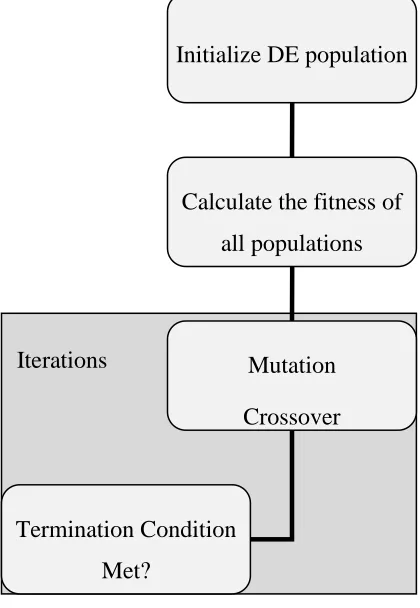
Initialization of the algorithm occurs once the initial vector population is chosen at random from an assumed parameter range (i.e. a range of integers from -10 to 10). Alternatively, if the preliminary solution is known, the population vector is populated using a normally distributed random deviation to the nominal solution, Xnom,0. The initially generated population (Xi,0)is perturbed using mutation and crossover, leading to the evolution of a new trial population. A selection process takes place to determine the fittest population of the two. The fittest population is selected as the initial population for the subsequent generation. This process continues iteratively until a termination
condition is met. Fig 1.1 summarizes the main components of the algorithm.
Iterations
Initialize DE population
Calculate the fitness of all populations
Mutation Crossover
Selection
Termination Condition Met?
The initialization strategies currently used with the DE address two specific scenarios: certainty or uncertainty. When preliminary information is available with certainty, the algorithm may be initialized using the nominal solution as discussed (Lampinen et al., 2005). Otherwise, if preliminary information is not available, the initialization will have to rely on a range of possible solutions (Lampinen et al., 2005).
However, when vague preliminary knowledge of the problem domain is available, neither method for initialization is ideal. Using such vague information to assume a nominal solution incorrectly implies more certainty than available. Alternatively assuming a range of solutions accounts for the uncertainty but may not utilize all available information to represent it correctly. The more knowledge one includes, the less uncertain will be the initialization and, consequently, the optimization.
The fuzzy set theory (Zadeh, 1965) offers a means to address the quantification of uncertainty from the available vague information. A brief overview of the main concepts of this theory is given in Appendix A. The fuzzy set theory offers unique possibilities for modifications of the traditional fundamentally stochastic DE algorithm. Some fuzzy practitioners have been already involved with evolutionary optimization. Some have utilized the existing algorithm to develop fuzzy models, like Kisi (2004) who found the parameters of membership functions for daily suspended sediment modeling. Others have joined the ongoing research that has resulted in modifications of the classic DE algorithm, such as Liu and Lampinen (2004). They proposed a fuzzy adaptive parameter control algorithm, based on feedback from the search behavior, to address the sensitivity of the DE to control parameter settings.
more efficient search strategy. For convenience, the novel algorithm is implemented into optimization decision support system software.
1.1
Organization of the Thesis
This thesis is organized into four additional chapters. Chapter Two gives an overview of the methodological background of the classic differential evolution algorithm strategy, as well as of several other selected strategies. An illustrative numerical example of the classic differential evolution algorithm is also presented here. The chapter also contains guidelines for setting the DE control parameters based on empirical evidence; in addition, the fuzzy adaptive differential evolution methodology is detailed. Constraint handling methodologies are also overviewed, including the random and bounce-back
reinitialization approach for dealing with search space constraints and the penalty function method for dealing with feasible space constraints. Lastly, the methodology for the novel fuzzy differential evolution (FDE) algorithm for initialization and mutation is proposed. This approach uses prior knowledge of the problem domain for guiding the search towards the optimal solution. A numerical example of the fuzzy differential algorithm is also presented for illustrative purposes.
Chapter Three outlines the optimization decision support system software package developed by integrating all the features discussed in the methodology. An illustrative example is used to demonstrate the decision support system and a typical procedure required to find the optimal solution. Chapter Four details two applications of the novel fuzzy differential evolution algorithm. Included is the application of a set of standard benchmark functions, used to compare the performance of the classical DE algorithm (in terms of convergence speed) with the proposed FDE algorithm. The second example is a practical application of the proposed algorithm using a reservoir operation case study. The final Chapter Five is a summary of key contributions/findings with a view into possible directions for future research aimed at expanding the FDE concept.
Chapter 2
2
Methodology
In the following sections of this chapter an overview of the original differential evolution algorithm is presented, alongside several other common variants. Presented is also an overview of control parameter selection strategies. Additionally, the approach for handling constraints is detailed. Lastly, the contribution of this thesis, the novel fuzzy differential evolution algorithm methodological background is detailed.
2.1
Differential Evolution Algorithm
The DE algorithm after initialization has three main operations: (I) mutation, (II) crossover and (III) selection before finishing due to a termination condition. The fundamental idea behind DE is a specific way of generation of trial parameter vectors. This is achieved using mutation and crossover to generate new trial parameter vectors. Selection then determines which of the vectors will survive to be used in the next generation. Through repeated cycles of mutation, crossover and selection, DE is able to guide the search towards the vicinity of the global optimum.
The original DE algorithm scheme proposed by Storn and Price (1995) gave the working principles of DE. Subsequently, contributions of other variants or strategies have been made and continue to be made. Different DE strategies can be adopted in the DE
algorithm depending upon the type of problem to which DE is applied. The strategies can vary based on the vector to be perturbed, the number of difference vectors considered for perturbation and the type of crossover used.
using any randomly chosen vector. The y variable is the number of difference vectors considered for the perturbation of x. Hence if it is a single vector difference, three distinct randomly chosen vectors are required, because the weighted differential of two vectors is added to the third one. Lastly, z stands for the type of crossover used: either exponential (exp) or binomial (bin). If exponential crossover is chosen, the crossover is performed on the D variables in one loop until it is within a given bound represented by the control parameter CR (crossover rate). The first time a randomly picked number between 0 and 1 exceeds the CR value, crossover is halted and the remaining D variables are left intact. If the crossover is binomial, it is performed on each of the D variables whenever a
randomly picked number between 0 and 1 is within the CR value. Therefore for high values of CR, the exponential and binomial crossover methods yield similar results. In practice, the binomial crossover approach is used more frequently.
The performance of the various DE variants is highly dependent on the given problems, so that a suitable one for any particular problem may not be as suitable for another. This assertion is reinforced by the no free lunch theorem (NFL) which states that no single search algorithm exists that can solve all problems efficiently (Wolpert and Macready, 1997). With that in mind, the importance and amount of research into strategies and control parameters for the best convergence efficiency is hardly surprising. The strategy and control parameter selection with best performance for a given problem is typically unknown, though some guidance exists. The usual approach is trial-and-error. However, the original DE algorithm strategy, under the notation DE/rand/1/bin by Storn and Price (1995), appears to be the most successful and the most widely used. The following presentation is based on the original/classic DE scheme.
2.1.1
DE Population Initialization
A common starting point with implementing any evolutionary algorithm is the
first issue. The latter, which is related to population size, a critical parameter of DE, will be focused on in Section 2.3.
As stated in earlier sections, each gene of each individual is initialized using a uniform random generator within the search ranges. This concept is the same for all evolutionary algorithms and DE is no exception. Let us assume that we are working in a
D-dimensional problem. Then each individual of the DE population, PG, would be a D-dimensional vector which can be initialized as follows:
(2.1)
Such that denotes the tth gene (t =1,2,…,D) of the ith individual (i =1,2,…, NP) in generation G =1. Randt(a,b) denotes the uniform random number generator that returns a uniformly distributed random number from [a, b]. The subscript in Randt is used to clarify that a separate random number is drawn for each gene in each individual. LBt and
UBt denote the lower and upper limits of the search ranges for gene j, respectively. It is
A population vector with its gene and individual components is presented in Table 2.1 for clarity.
Table 2.1. Population vector matrix for each generation
Gene
Individual
1 2 D
1 X1,1 X1,2 X1,D
2 X2,1 X2,2 X2,D
NP XNP,1 XNP,2 XNP,D
2.1.2
Mutation
DE derived its name from the mutation operator it applies to mutate its individual. Mutation is the first of two main operators (the other being crossover) required to alter the “genetic code” of current individuals to improve diversity of a population. A
mechanism for evolving the population of vectors is essential. There is the possibility that re-selection of vectors already chosen can occur along with other vectors being omitted from the search. Vectors that are not chosen are deprived of passing on potential diversity to the next generation. Re-selection of vectors causes the potential to lose diversity in the next generation due to over sampling of the same vector. DE ensures that this does not happen by comparing vectors from competing populations by their index.
The mutation operator is called “differential mutation” and generates the mutated individual (also known as mutated vector) mi,G+1,for the principal parent (also known as target vector) xi,G according to the following equation (Storn and Price, 1997):
( )
where F ϵ [0, 2] is a real number that controls the amplification of the difference vector (xr2, G-xr3, G), while r1, r2, r3 ϵ [1, NP] represent randomly chosen indexes, where r1 corresponds to the base vector. The indexes have to be different from each other and from the running index i. That way, a parent pool of four individuals is required to breed an offspring.
2.1.3
Crossover
To complement the differential mutation search strategy, DE then uses a crossover operation, in which the mutated individual is mated with the principal parent and generates the offspring or “trial individual”. This crossover operation for classic DE as reviewed here is known as binomial crossover.
The target vector xi,G is mixed with the mutated vector, mi,G, using the following scheme, to yield the trial vector (Storn and Price, 1997)
(2.3)
where
{
(2.4)
CR is the crossover constant ϵ [0, 1] (to be specified by the user), t =1, 2,…, D and randt
is the tth evaluation of a uniform random generator number ϵ [0, 1]. Lastly, to guarantee that a new altered population vector is produced, a randomly chosen index rni ϵ
2.1.4
Selection
DE uses a selection mechanism to ensure that the individuals promoted to the next generation are strictly those with the best fitness values in the population. A knockout competition is played between each individual (target vector) and its offspring (trial vector) . The survival criteria can be described as follows (Storn and Price, 1997):
{ ( ) ( )
(2.5)
where indicates the objective function that is being optimized (minimized here). This one-to-one selection mechanism ensures that the selected individuals are strictly those with the best fitness values in the population. That is to say, the trial vector ui,G+1 must yield a better fitness value than xi,G, for xi,G+1 to be set to ui,G+1; otherwise, the old value xi,G is retained. Practicing this one-to-one selection mechanism thus enables DE to exercise elitism on its population. Due to its positional elitism strategy it discards an offspring which is better than most of the current population but worse than its parent. However, such rejected individuals could be useful to accelerate the search for the global optimum (Iba and Noman, 2012).
2.1.5
Termination
Termination of the algorithm ideally takes place after the global optimum is achieved, but this may not always be the case. Frequently, termination of the algorithm is a
terminate. Additionally, feedback provided by the objective function can determine that no further optimization is possible. For example, if the optimization stalls and thus many subsequent objective function values are the same, the algorithm may be terminated. Also, human monitoring can determine when optimization is over.
2.1.6
Illustrative Example of Classic DE Algorithm
A simple numerical example adopted from Arunachalam (2008) is presented to illustrate the classic DE algorithm. Let us consider the following objective function for
optimization:
(2.6)
The initial population is chosen randomly between the bounds of decision variables, in this case x1, x2 and x3 ϵ [0, 1]. The population along with its respective objective function values is shown in Table 2.2. The first member of the population, “Individual 1”, is set as the target vector.
Table 2.2. An illustrative example
Population Size NP=6 (user defined), D=3
Individual 1 Individual 2 Individual 3 Individual 4 Individual 5 Individual 6
x1 0.68 0.92 0.22 0.12 0.40 0.94
x2 0.89 0.92 0.14 0.09 0.81 0.63
x3 0.04 0.33 0.40 0.05 0.83 0.13
f(x) 1.61 2.17 0.76 0.26 2.04 1.70
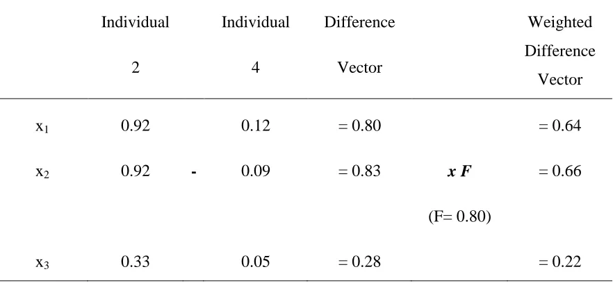
Table 2.3. Calculation of the weighted difference vector for the illustrative example
Individual 2 Individual 4 Difference Vector Weighted Difference Vector
x1 0.92 0.12 = 0.80 = 0.64
x2 0.92 - 0.09 = 0.83 x F
(F= 0.80)
= 0.66
Table 2.4. Calculation of the mutated vector for the illustrative example
Weighted Difference
Vector
Individual
6
Mutated
Vector
x1 0.64 0.94 = 1.58
x2 0.66 + 0.63 = 1.29
x3 0.22 0.13 = 0.35
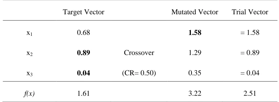
The mutated vector does a crossover with the target vector to generate the trial vector, as shown in Table 2.5. This is carried out by (1) generating random numbers equal to the dimension of the problem (2) for each of the dimensions: if random number > CR; copy the value from the target vector, else copy the value from the mutated vector into the trial vector. In this example, the crossover constant CR is chosen as 0.50.
Table 2.5. Generation of the trial vector for the illustrative example
Target Vector Mutated Vector Trial Vector
x1 0.68 1.58 = 1.58
x2 0.89 Crossover 1.29 = 0.89
x3 0.04 (CR= 0.50) 0.35 = 0.04
f(x) 1.61 3.22 2.51
which completes one generation. Once the termination criterion is met, the algorithm ends.
Table 2.6. New population for the next generation in the illustrative example
New Population for the Next Generation
Individual 1 Individual 2 Individual 3 Individual 4 Individual 5 Individual 6
x1 0.68
x2 0.89
x3 0.04
f(x) 1.61
2.2
Selected Differential Evolution Algorithm Variants
In addition to the classical DE strategy DE/rand/1/bin, there are many derivative strategies for perturbation of the population vectors. The motivation to develop such strategies has come from the fact that no single perturbation method has turned out to be best for all problems (Chakraborty, 2008). Discussed here is DE/best/1/bin and
DE/current(local)-to-best/1/bin, two very popular mutation strategies for addressing optimization problems that the original strategy may not perform adequately. These two strategies benefit in faster convergence by incorporating the best solution information in the evolutionary search. However the best solution information may also cause problems such as premature convergence due to the resultant decreased population diversity.
2.2.1
DE/best/1/bin
scheme and this variant is based on the perturbation of the vectors. In the DE/best/1/bin scheme only the mutation component of the algorithm is modified with respect to the original, incorporating information from the objective function. Instead of randomly populating the base vector from randomly chosen indexes in the current generation (as in the original scheme), in DE/best/1/bin the algorithm always selects the best-so-far vector (best) as the base vector, adds a single scaled vector difference to it, then creates a trial vector by uniformly crossing the resulting mutant with the target vector. Thus the base vector always has the best (fittest) objective function value in the current population. Compared to random base vector selection, using the best-so-far vector lowers the diversity of the pool of potential trial vectors (Lampinen et al., 2005).
The above description is expressed in the formula below, where for each target vector xi,G, a mutation vector mi,G is generated according to (Price, 1996)
( )
(2.7)
where F ϵ [0, 2] is a real number that controls the amplification of the difference vector (xr1, G-xr2, G) and r1, r2 ϵ [1, NP] represent randomly chosen indexes. The indexes have to be different from each other and from the running index i so that NP must be at least three. Xbest,G corresponds to the best vector from the best population solution in the current generation.
2.2.2
DE/local-to-best/1/bin
This DE variant computes the difference between the ith member (target vector) and the best-so-far member of the current population (Lampinen et al, 2005). This method attempts to balance robustness with fast convergence and is a popular choice in most studies of DE.
( ) ( )
2.3
Setting Control Parameters
Control parameters have already been briefly mentioned, but due to their importance to the performance of DE algorithms a more detailed explanation is given here. The values of population size (NP), crossover constant (CR) and weighing factor or mutation scale factor (F) are fixed empirically, following certain heuristics. Proper tuning of these parameters is essential for the reliable performance of the algorithm. Trying to tune these three main control parameters and finding bounds for their values has been a topic of intensive research (Chakraborty, 2008).
The mutation scale factor F controls the speed and robustness of the search. A lower value for F increases the convergence rate but it does so at the risk of getting stuck into a local optimum and therefore failing to find the true global solution. Parameters CR and NP have a similar effect on the convergence rate as F. High values of CR favor a higher
mutated element crossover to current elements; as a result, the mutation factor F has a greater impact on the search. As well, an increased value of NP increases the diversity of the population and with it the potential to find the true optimal solution from the greater search space but at the cost of longer computation time.
The control parameter selection is a difficult task due to their interdependence with each other and the fact that some objective functions are sensitive to proper settings (Liu and Lampinen, 2002). Traditionally, the control parameters have been held fixed during the whole execution of the algorithm.
The rule-of-thumb values for the control parameters given by Storn and Price (1997) for F is usually between 0.5 and 1.0 and CR between 0.8 and 1.0. These authors have
parameters for each problem setting. As a result of the difficulty of setting appropriate control variables, research has focused on finding parameters such as F and CR settings automatically (Zhang and Sanderson, 2009).
For example, Brest et al. (2006) proposed a self-adaptive version of DE that
automatically adjusts its control parameters F and CR at an individual level. Likewise, a feedback update rule for F was proposed by Zaharie (2003), designed to maintain the population diversity at a given level, thereby reducing a premature convergence of the search. Fuzzy adaptive differential evolution (FADE), introduced by Liu and Lampinen (2004), is another example of methods that determine the control parameters
2.3.1
Fuzzy Adaptive Differential Evolution
Fuzzy logic is a means of transforming linguistic knowledge into a mathematical model. It has been used extensively in the field of automatic control where it succeeded in the modeling and control of many systems that cannot be described using classical control techniques. Therefore fuzzy logic offers a means of rendering control parameters more adaptive to each optimization problem. The result of implementing fuzzy adaptive differential evolution (FADE) is a more efficient search (a lesser number of function evaluations) (Liu and Lampinen, 2004).
FADE uses a fuzzy knowledge-based system to adapt dynamically the control parameters F and CR for the mutation and crossover operations. It uses a series of fuzzy rules
developed based on existing empirical evidence to infer appropriate values of F and CR for each generation, based on parameter and objective function difference vector from subsequent generations. The adaptive parameters using FADE accelerate the convergence velocity of DE.
FADE uses Mamdani’s inference method to establish the control parameter (Mamdani and Assilian, 1975). Mamdani’s fuzzy inference method is detailed in Appendix B.
and
(2.10)
where PC is called the parameter vector change in magnitude and is transformed into the range of [0,1] as d11 and the range of [0,2] as d21; FC is called the function value change and is transformed into [0,1] as d12 and [0,2] as d22;
is the ith component of the function value vector for the nth generation, i = 1,2,…,NP; is the component in the
ith row and jth column of the parameter matrix XNP×D for the nth generation, i =
1,2,…,NP, j = 1,2,…,D; n is the generation index; NP and D represent the population size and dimensionality of the problem, respectively.
Actual input values for the fuzzy inference are the numerical values as stated in Eq. (2.10); output variables are the parameter values for F and CR, whose ranges are sets of real numbers.
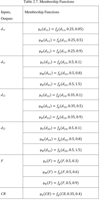
Table 2.7. Membership Functions
Inputs, Outputs
Membership Functions
d11
d21
d12
d22
F
The values of F and CR are adapted based on d11, d12, d21, d22 and a series of fuzzy rules used to describe the characteristics of the system. There are a total of 18 rules for determining F and CR values, 9 each. Each rule has two inputs and one output which represent the mapping from the input space to the output space. The “9×2” rules are given in Table 2.8.
Table 2.8. The Fuzzy Rules
Rule Fuzzy Sets
di1 di2 F or CR
1 S S S
2 S M M
3 S B B
4 M S S
5 M M M
6 M B B
7 B S B
8 B M B
9 B B B
Finally, the adaptive parameters may be found given the supplied information and Mamdani’s inference in conjunction with a centroidal defuzzification technique.
Defuzzification is mapping from a space of fuzzy output into a space of real output. The result is a single number y* which represents the value of the mutation amplification F or crossover factor CR.
2.4
Constraints
Constrained optimization problems, especially nonlinear optimization problems, where objective functions are to be optimized under given constraints, are very important and frequently appear in the real world. For this reason, DE has had significant research invested into dealing with optimization problems, with inequality constraints, equality constraints, as well as upper and lower bound constraints (Chakraborty, 2008; Lampinen et al., 2005). Constrained optimization problems are mathematically expressed as
(2.11)
Where x = (x1, x2,…,xk) is a k-dimensional vector, f(x) is an objective function, gj(x) ≤ 0 and hj(x) = 0 are n inequality constraints and m equality constraints, respectively. Functions f, gj and hj are linear or nonlinear real-valued functions. Values ui and li are upper and lower bounds of xi, respectively.
search space in which every point satisfies upper and lower boundary constraints denoted by S(F). Fig. 2.1 shows graphically the search space and feasible region.
Figure 2.1. Search space and feasible region.
2.4.1
Search Space Constraint
After initialization, the algorithm may produce mutated vectors in subsequent generations that fall outside of the initial search boundaries. The initial search bounds give
information on the assumed feasible search space for the problem and thus can be used to define the low and high limits put on each individual. In some cases it may be desirable for the search to be able to have the freedom to surpass the set bounds. This may be in instances where the search space is improperly preset due to a lack of knowledge about the problem domain. However, in all other cases this is harmful and non-desirable. For example, a negative value for discharge for a reservoir operation problem is absolutely inadmissible; as such, the lower bound constraints must be maintained, LBt = 0.
{
(2.12)
The other approach to regularize infeasible mutant vectors is called bounce-back. Bounce-back replaces the offending parameter with another, chosen between the boundary and the base vector.
If the mutated vector exceeds the lower bound:
( )
(2.13)
If the mutated vector exceeds the upper bound:
( )
(2.14)
Bounce-back may be preferred over random reinitialization as it is able to preserve the direction of the current search. As a result, the convergence speed using bounce-back may be favorable to random reinitialization.
2.4.2
Feasible Space Constraint
Some problems have constraint functions which cannot be dealt with utilizing the search space boundary constraints. The penalty function method is widely used for constrained optimization problems, not just in differential evolution algorithms but in other
optimization algorithms as well. The penalty function method transforms the constrained problem into an unconstrained one by penalizing infeasible solutions, in which a penalty term is added to the objective function for any violation of the constraints (Gen and Chen, 1997).
added on to the objective failing in order to compete with solutions without penalty in the selection process of DE. It needs to be emphasized that infeasible solutions may not be rejected outright in each generation, as they may provide much more useful information about optimal solution than some feasible solutions. The major concern is how to determine the penalty term so as to strike a balance between keeping some infeasible solutions and rejecting others. An overly low penalty term constant may keep too many infeasible solutions, whereas a very high penalty constant may reject all the solutions preventing the optimization from convergence to an optimal solution.
Careful selection of the penalty control parameters is required for the proper convergence to a feasible optimal solution and is very much problem-dependent.
The differential evolution algorithm is modified to take account of constraint functions using the penalty function method. The fitness function modified for taking account of the penalty function may be expressed as follows (Gen and Chen, 1997):
(2.15)
where x represents the genes parameter vector, f(x) the objective function of the problem and p(x) the penalty function. For an optimization problem, it is required that
(2.16)
To demonstrate how the function in Eq. (2.16) may be formulated consider the example problem where the initial parameter values for x1 and x2 are found to be 5 and 2
(2.17)
The above two constraints would be transformed to an unconstrained problem and multiplied by a penalty constant as follows:
(2.18)
2.5
Fuzzy Differential Evolution Algorithm
The novel fuzzy differential evolution (FDE) algorithm proposed here allows a novel approach for additional problem domain information to be communicated to the DE algorithm for optimization. Doing so results in better overall performance.
Differential evolution is fundamentally a stochastic based algorithm. The name FDE may suggest a full deviation to the fuzzy domain. However, this is not the case. The proposed method may be better described as a stochastic and fuzzy hybrid. The (I) initialization and (II) mutation procedures are modified so that they utilize both, the fuzzy and the stochastic theory.
2.5.1
Initialization
Initialization is done in order to seed the population NP, D-dimensional parameter vector of the algorithm. Traditionally performed through using randi ϵ [0, 1], a uniform
probabilistic distribution to randomly select within upper (bU) and lower bounds (bL) agents is to be carried through subsequent algorithm components:
(2.19)
Membership functions describe the degree of membership or truth in each value
corresponding to a parameter. Many shapes of membership functions may be used. In this paper, for illustration and convenience, we are limiting our discussion to the triangular membership function. A fuzzy triangular number A = (a1, a2, a3) can be represented by an ordered triplet or by a triangular membership function
{
(
) (
)
(2.20)
Fig. 2.2 shows a triangular membership function defined by Eq. (2.20) where a2 holds the highest degree of membership in x (membership, µ = 1) comparatively a1 and a3 hold no degree of membership (µ = 0). Within the FDE algorithm a1 and a3 are called the initial parameter range while a2 is called the focus or target parameter.
Figure 2.2. Triangular fuzzy membership function.
µ
1.0
0.5
0.0
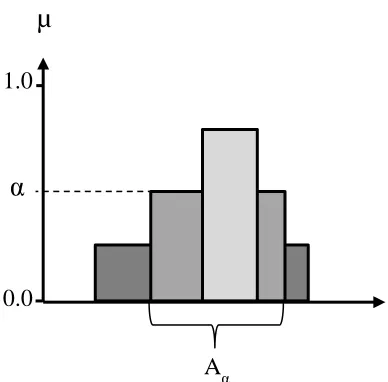
Alpha-cuts are mostly used to extract information from a membership function and are rarely used for defuzzifying the fuzzy sets (converting fuzzy numbers into crisp form). The alpha-cut describes a fuzzy set using a set of sharp sets. The main idea is to fix a certain membership degree α and thus to obtain a crisp set, which is defined as the set of values that have a membership degree higher or equal to α. Fig. 2.3 illustrates the concept of alpha-cuts. The membership function is cut horizontally at a finite number of regular α-levels, or cuts, between 0 and 1. This process generates a number of crisp interval sets as shown in Fig. 2.4.
Figure 2.3. The alpha-cut method schematic.
µ
1.0
α
0.0
x
α – level cutAα
Figure 2.4. The alpha-cut intervals schematic.
Taking an arbitrary alpha-cut ϵ [0, 1] in A (a triangular fuzzy number), a confidence fuzzy interval, Aα is obtained, defined as
(2.21)
Relating to FDE, parameters are described using triangular fuzzy numbers in the form of inputs for the triangular membership function. To start the algorithm, the initial
population vector needs to be generated from these membership functions. This is achieved by using the alpha-cut method NP times at random α-levels to create alpha-cut intervals for each parameter. This allows for a unique individual to be generated NP times from the same parameter membership function input (fuzzy number). The alpha-cut interval is assumed to belong to a unique fuzzy number. In essence, the initial fuzzy number is used to seed NP unique incomplete fuzzy numbers defined only by a single discrete alpha-cut level.
The alpha-cut interval population vector, ,is found by modifying Eq. (2.21).
µ
1.0
α
0.0
(2.22)
Where i = 1, 2,…, NP and α is the alpha-cut level such that it is equal to a uniform random number generated, randi ϵ[0,1]i. and are the lower and upper interval
bounds for each alpha-cut. The parameters a1, a2, a3 are the values representing the fuzzy number triplet for each individual parameter.
In singular value form, the alpha-cut intervals are converted to the familiar population vector where neutral preference is given to the upper and lower intervals
(2.23)
In order for a unique singular value to be generated, an asymmetrical triangular membership function must be used.
2.5.2
Mutation
FDE/rand/1/bin. A similar modification to the one presented here could be performed for several other DE variants available, but that is beyond the scope of this paper.
DE/rand/1/bin defines the weighted differential of two different randomly chosen vectors and is used to perturb another randomly chosen vector, creating a mutated vector. This process is mathematically expressed in Eq. (2.2).
The mutation vector mathematical expression in Eq. (2.2), transformed using alpha-cut intervals (from initialization and subsequently), has the following form:
( ) (2.24)
Utilizing fuzzy interval arithmetic properties for addition and subtraction (Bojadziev and Bojadziev, 1995),
(2.25)
and substituting for Eq.(2.24) yields the lower and upper mutation vector interval bounds:
( )
Where i = 1, 2,…, NP. The alpha-cut population vector interval , is represented by discrete endpoints ( ) for levels , , . These levels may equal to each other or they may be different. However, as seen in Eq. (2.25) the alpha-cut level α must be the same throughout in order to proceed with interval arithmetic. This is likely not the case in the initialization stage where unique alpha-cut intervals are generated.
Each of the alpha-cuts for the purpose of the FDE algorithm represents a unique fuzzy number. These fuzzy numbers are incomplete, because they are defined by a single alpha-cut level (Bojadziev and Bojadziev, 1995). In order to perform interval arithmetic at the same alpha-cut level, redefining of incomplete fuzzy numbers is required. Redefining allows incorporating levels not given initially (Bojadziev and Bojadziev, 1995).
The mutated alpha-cut intervals vector can be expressed in the traditional singular value form:
(2.27)
2.5.3
Illustrative Example of FDE Algorithm
The same simple numerical example that was used to illustrate the original DE algorithm is presented here to illustrate the FDE algorithm. Let us consider the following objective function for optimization:
(2.28)
The initial population is chosen by taking NP (defined as 6) random alpha-cuts of a fuzzy membership function for each decision variable; in this case x1, x2 and x3 are defined by the same triangular fuzzy membership function triplet (0, 1, 3). Therefore, the initial parameter range is ϵ[0,3] while the target or focus is 1.
= 1.8
(2.29)
The fuzzy interval in Eq. (2.29) is transformed to a singleton using Eq. (2.23).
( ) (2.30)
The population along with its respective objective function values is shown in Table 2.9. The first member of the population “Individual 1” is set as the target vector.
Table 2.9. An illustrative example
Population Size NP = 6 (user defined), D = 3
Individual 1 Individual 2 Individual 3 Individual 4 Individual 5 Individual 6 Fuzzy Interval Fuzzy Interval Fuzzy Interval Fuzzy Interval Fuzzy Interval Fuzzy Interval
x1 1.20 0.60,1.80 1.11 0.77,1.46 1.05 0.90,1.20 1.19 0.61,1.77 1.28 0.45,2.11 1.14 0.72,1.67
x2 1.11 0.79,1.42 1.26 0.48,2.04 1.14 0.73,1.55 1.49 0.03,2.94 1.18 0.63,1.73 1.06 0.89,1.22
x3 1.44 0.12,2.76 1.12 0.76,1.48 1.02 0.97,1.07 1.30 0.39,2.22 1.09 0.82,1.37 1.16 0.68,1.63
f(x) 3.74 3.49 3.20 3.98 3.55 3.36
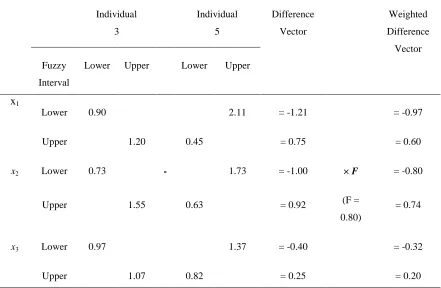
Table 2.10. Calculation of the weighted difference vector for the illustrative example
Individual 3 Individual 5 Difference Vector Weighted Difference Vector Fuzzy Interval
Lower Upper Lower Upper
x1
Lower 0.90 2.11 = -1.21 = -0.97
Upper 1.20 0.45 = 0.75 = 0.60
x2 Lower 0.73 - 1.73 = -1.00 × F
(F = 0.80)
= -0.80
Upper 1.55 0.63 = 0.92 = 0.74
x3 Lower 0.97 1.37 = -0.40 = -0.32
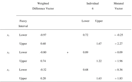
Table 2.11. Calculation of the mutated vector for the illustrative example
Weighted Difference Vector
Individual 6
Mutated Vector
Fuzzy Interval
Lower Upper
x1 Lower -0.97 0.72 = -0.25
Upper 0.60 1.67 = 2.27
x2 Lower -0.80 + 0.89 = 0.09
Upper 0.74 1.22 = 1.96
x3 Lower -0.32 0.68 = 0.36
Upper 0.20 1.63 = 1.83
The mutated vector fuzzy intervals can be expressed in traditional single value form using Eq. (2.27). The mutated vector in single value form is given in Table 2.12.
Table 2.12. Interval to single value mutated vector calculation
Upper Fuzzy Interval Bound
Lower Fuzzy Interval Bound
Sum Mutated Vector
x1 2.27 -0.25 = 2.22 = 1.11
x2 1.96 + 0.09 = 2.05 ×0.5 = 1.03
The mutated vector does a crossover with the target vector to generate the trial vector as shown in Table 2.13. This is carried out by (1) generating random numbers equal to the dimension of the problem (2) for each of the dimensions: if random number> CR; copy the value from the target vector, else copy the value from the mutated vector into the trail vector. In this example, the crossover constant CR is chosen as 0.60.
Table 2.13. Generation of the trial vector for the illustrative example
Target Vector Mutated Vector Trail Vector
x1 1.20 1.11 = 1.11
x2 1.11 Crossover 1.03 = 1.03
x3 1.44 (CR = 0.60) 1.10 = 1.44
f(x) 3.74 3.24 3.58
Table 2.14. New population for next generation for the illustrative example
Population Size NP = 6 (user defined), D = 3
Individual 1 Individual 2 Individual 3 Individual 4 Individual 5 Individual 6 Fuzzy
Interval
Fuzzy Interval
Fuzzy Interval
Fuzzy Interval
Fuzzy Interval
Fuzzy Interval
x1 1.11 -0.25,2.27
x2 1.03 0.09,1.96
x3 1.44 0.12,2.76
Chapter 3
3.1
Decision Support System Software Package
The DE algorithm has been implemented in the form of a convenient decision support system (DSS) called the Differential Evolution Optimizer (DEO). The decision support system integrates, alongside the classical algorithm, key differential evolution features discussed in the methodology, such as fuzzy differential evolution and the ability to deal with constraints. DSS is developed to provide a convenient optimization software package with a friendly graphical user interface for the MS Windows operating system. DSS provides easy access and all the practical benefits to an efficient optimization algorithm for less technical individuals. DEO was programmed in C# and the code, as well as the installation files, have been provided electronically with the thesis. Brief overviews of the supplementary files included with this thesis are in Appendix C.
In this chapter, a helpful user guide of DEO is presented to review the key features and the process involved in inputting and reading the results from a defined optimization problem. In addition to the user guide, an illustrative example problem is used as a step-by-step guide of the typical procedure towards finding an optimal solution using the DSS.
3.2
Differential Evolution Optimizer Overview
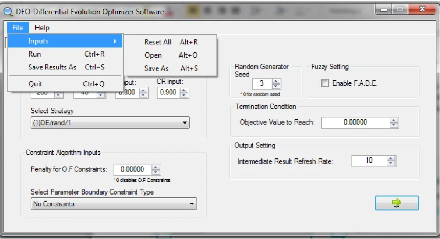
Once the Differential Evolution Optimizer DSS is run, an execution window like the one shown in Fig. 3.1 should be displayed. Upon starting the DEO decision support system the user is greeted with the “Algorithm Inputs” window tab open. As the user fills in the appropriate input fields he/she is able to proceed to the “Optimization Inputs” window and finally the “Optimization Results” window. These will be reviewed in the
Figure 3.1. Interface of DEO menu.
Fig 3.1. shows the interface of the menu strip in the top left corner of the program window with two options “File” and “Help” (the documentation you are now reading). Upon clicking “File”, the user is presented with the option for “Inputs”, to “Run” the optimization, “Save Results” of the optimization once a problem has been optimized and the option to “Quit”, i.e. to close the program.
Selecting “Inputs” will further open additional menu options: “Reset All” reverts all input parameters to default; “Open” automatically fills the input requirements by
prompting the user to select past saved (.deo extension) input files; and “Save As” saves the current inputs and prompts the user to name the file and the file will be saved with a .deo extension.
3.2.1
Algorithm Inputs
The main body of the algorithm inputs window contains multiple interface inputs
pertaining to setting up the differential evolution algorithm. Fig. 3.2 shows the algorithm inputs window. The inputs are labeled numerically for reference within this section.
Figure 3.2. Algorithm inputs window.
Each number in Figure 3.2 corresponds to a detailed explanation given below.
1. Included under the main algorithm inputs heading are four user defined control parameters for the differential evolution algorithm. They are detailed below.
Generation input is the number of iterations (generations) the algorithm will go through to find the optimal solution before termination. The more generations given, the greater the accuracy of the final result may be to the true optimal solution at the expense of more computation time.
NP input is the number of parents which, as a guideline, may be selected to be 10 times the number of parameters of the objective function.
speeding up convergence. Empirical evidence suggests that increasing NP above 40 does not significantly influence the convergence rate.
F input, the weighing factor F [0, 2] controls the amplification of differential variation; to begin with, a value of 0.8 is suggested.
CR input The crossover weight CR [0,1] probabilistically controls the amount of recombination; initially a value of 0.9 is suggested.
These parameters are of significance for the accuracy and convergence time required. Therefore, a proper selection is very important. Adequate selection of each of the parameters may differ from problem to problem and may require some trial and error in selection. The user can choose to enter the values directly within the textbox or increment the number by clicking either the up or down arrow beside the textbox. 2. Differential evolution has a specialized nomenclature that describes the selected
strategy for optimization. The nomenclature and the methodology for the variants included within DEO were discussed in detail in Chapter 2. DEO has 4 available strategies that are accessed through a dropdown menu:
i. DE/rand/1: The classical version of DE.
ii. DE/best/1: Tailored for small population sizes and fast convergence. Dimensionality should not be too high.
iii. DE/local-to-best/1: A version which has been used by numerous scientists. Attempts a balance between robustness and fast
convergence.
3. This DSS uses the penalty function method (discussed in Chapter 2) in order to deal with constraints on the feasible space for the objective function. The penalty function method is comprised of the optimization of the objective function with the addition of the constraint violation function (the sum of the violation of all constraint functions). The main challenge of the penalty function method lies in the difficulty of selecting an appropriate value for the penalty coefficient that adjusts the strength of the penalty. The user is required to provide the penalty function coefficient to be used for all the objective function constraints; if the user does not wish to use any constraints on the objective function, a penalty
coefficient of zero should be used. When dealing with a minimization problem, the penalty coefficient must be a positive value; conversely, when it is a
maximization problem, the coefficient must be a negative value. This assures that any constraint violations will indeed penalize the optimization solution and not make it better.
The user can choose to enter the values directly within the textbox or increment the number by clicking either the up or down arrow beside the textbox.
5. The user is given the option of selecting the seedvalue used by the random generator. This makes it possible to achieve the same results through multiple optimization runs, given that the same seed is used. Furthermore, an easier comparison between different control inputs can be achieved. If the user wishes for the seed to be random, a value of zero should be placed in the input field. The user can choose to enter the values directly within the textbox or increment the number by clicking either the up or down arrow beside the textbox.
6. The fuzzy settings allow the user to enable the FADE settings by clicking the checkbox. FADE stands for fuzzy adaptive differential evolution, as discussed in detail in Chapter 2. FADE optimizes the control parameters CR and F for each generation to increase accuracy and convergence speed by referencing a database corresponding to fuzzy rules based on empirical findings. As a result, the user does not need to spend time selecting appropriate values for CR and F, as these values are only used for the initialization of FADE.
7. The termination condition input, VTR, is the value that will terminate the algorithm upon achieving. This feature is particularly useful for benchmark functions where the optimal objective function solution is known.
8. The output setting allows the user to select how the intermediate results should be displayed. For example if the input here is 10, the intermediate result outputs will be displayed every 10th iteration (generation).
3.2.2
Optimization Inputs
After clicking the next button on the algorithm inputs window the optimization inputs tab will open. Here, multiple interface inputs allow for the objective function to be defined—the boundary range for each parameter (used for initialization) and objective constraints (if any)—before finally proceeding with the optimization. Fig. 3.3 shows the optimization inputs window. Inputs are labeled numerically for reference within this section. At any point the user may choose to hit the green arrow to go back to the previous algorithm inputs window.
Figure 3.3. Optimization inputs window.
Each number in Figure 3.3 corresponds to a detailed explanation given below.
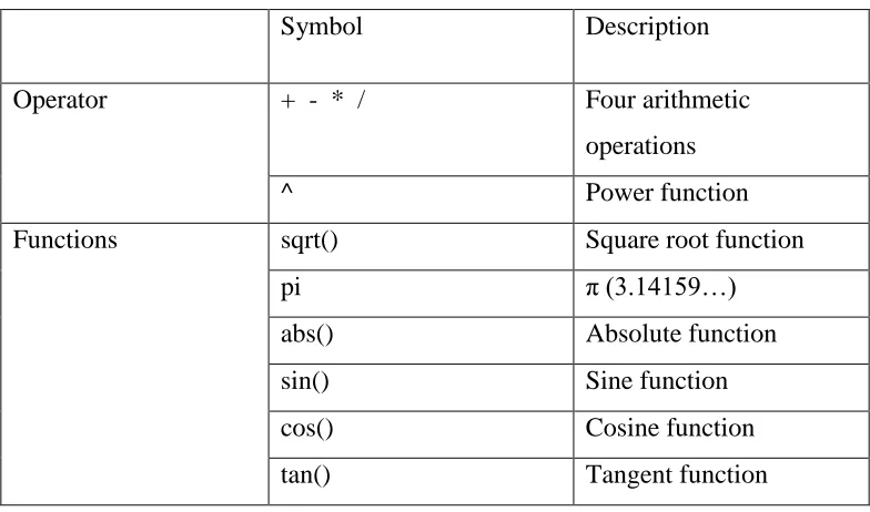
30 parameters and they must be defined as x1, x2 and so on. The operations and prebuilt functions which are recognizable by DEO are listed in Table 3.1.
Table 3.1. List of available functions
Symbol Description
Operator + - * / Four arithmetic
operations
^ Power function
Functions sqrt() Square root function
pi π (3.14159…)
abs() Absolute function
sin() Sine function
cos() Cosine function
tan() Tangent function
2. Once the objective function is provided, the user is required to define the search space used for initialization of the differential evolution algorithm.
a. If the user selected a traditional DE strategy, the user will be presented with this interface and will be required to give upper and lower bounds for each parameter defined in the objective function.
b. If the FDE strategy is selected, then the user will be presented with this interface and will need to define the triangular membership function for the boundary constraint of each parameter in the objective function. Once each parameter is defined, the user needs to click the Add button, this process is repeated until all have been defined. If at any point a mistake is made, the reset button can be clicked which will restart the search space definition process.
dropdown box enables the user to choose between inequalities to be used for the constraint. Available inequalities to choose between are: less than [<], greater than [>] or equal [=]. The right textbox accepts only crisp numerical values corresponding to the right-hand size of the constraints. Once each constraint is defined, the user needs to click the Add button, this process is repeated until all have been defined. If at any point a mistake is made the reset button can be clicked which will erase all the constraints.
4. Finally, once all the inputs have been provided, clicking the Run button will initiate the optimization. When Run is selected, the program may take some time to complete the optimization, depending on the complexity of the problem. Once the optimization is complete, the user will be presented with the optimization results window.
3.2.3
Optimization Results
Fig.3.4 details the optimization results window; the outputs are labeled numerically for detailed explanation below.
1. The intermediate output isproduced at the user defined interval, showing (from left to right) the current generation, the NFE (number of function evaluations) and the corresponding objective function value.
2. The optimization results are summarized here. These include the optimal parameter values, the optimal objective value and the generation and number of objective function evaluations it took to achieve the optimal results. The
computational time needed for optimization is also given in seconds.