A Theoretical Framework for Comparison of Data Mining Techniques

! " #

$#$ !% & &$

' ( ))) *

A Theoretical Framework for Comparison of Data Mining Techniques

Abhishek Taneja*

Assistant Professor, Dep’t. Of Computer Sc. & Applications Dronacharya Institute of Management & Technology,

Kurukshetra, India

[email protected]

R.K.Chauhan

Professor,Dep’t. Of Computer Sc. & Applications

Kurukshetra University, Kurukshetra Kurukshetra, India

[email protected]

Abstract: In recent years data mining has become one of the most important tool for extracting, manipulating data and establishing patterns in order to produce useful knowledge for decision making. Nearly all the worldly activities have ways to record the information but are handicapped by not having the right tools to use this information to embark upon the fears of future. In data mining the choice of technique depends upon the perceptive of the analyst. It is a daunting task to find out which data mining technique is suitable for what kind of underlying dataset. In this process lot of time is wasted to find the best/suitable technique which best fits the underlying dataset. This paper proposes a theoretical composition for comparison of different linear data mining techniques in a bid to find the best technique which saves lot of time which is usually wasted in bagging, boosting, and meta-learning.

Keywords: Data mining, Factor Analysis, Multiple Linear Regression (MLR) , Partial Least Square (PLS), Ridge Regression.

I. INTRODUCTION

Recently advancement in the data collection technology like bar code scanners, sensors in commercial and scientific domains have led to the collection of huge amount of data. This tremendous growth in datasets has pressed the creation of efficient data mining techniques that would lead to transform these datasets into useful knowledge and information. In that regard we have number of data mining techniques that would accomplish this difficult task. But all the techniques have got their own limitations and constraints. The choice of technique largely depends upon the perceptive of the analyst. In that regard lots of time is wasted in trying every singly prediction technique (bagging and boosting) and then comparing which technique best suits for the underlying dataset. The choice of technique plays a large role in the uncertainty of a model. When nonlinear data are fitted to a linear model, the solution is usually biased. When linear data are fitted to a non linear model, the solution usually increases the variance. Hence with the arrival of improved and modified prediction techniques there is the need for the analyst to know which prediction technique suits for a particular type of data set thus saving lot of time by preventing bagging, boosting, and meta-learning.

Relatively little has been published about the theoretical foundations for comparison of data mining techniques. First of all one has to answer the questions such as “Why we need such a theoretical foundation for comparison of data mining techniques?” Data mining is an applied area, with so many techniques available even for doing the same task. Particularly in this paper we would like to focus on linear predictive data mining techniques.

There are many different criteria to use to evaluate a statistical or data-mining model. So many, in fact it can be a bit confusing and at times seem like a sporting event where proponents of one criterion are constantly trying to prove it is the best. There is no such thing as a best criterion. Different criteria tell you different things about how a model behaves. In a given situation one criterion

may be better than others but that will change as situations change. Our recommendation, as with many other tools, is to use multiple methods and understand the strength and weaknesses of each method with the problem you are currently faced with. Many of criteria are slight variation

of another and most have residual sum of squares (RSS) in them in one manner or another. The differences may be slight but can lead to very different conclusions about the fit of a model.

II. LITERATURE REVIEW

The problem of choosing a new data mining technique comes when the analyst has no knowledge of the new data set. Selection of the best technique requires the deep understanding of the data modeling technique and their advantages and disadvantages with some superficial knowledge of the underlying dataset being used for process model.

near infrared instrument statistical calibration using only (root mean square error) RMSE as model comparison criteria. In year 2009, Hassan, Al et.al compared ridge regression and PCR using MSE as model comparison criteria [6]. In year 2009 Noori R. et.al compared neural network and principal component regression analysis to predict the solid waste generation in Tehran. They used correlation coefficient and average absolute relative error indices for model evaluation [7]. In year 2002, Yeniay et.al compared PLS with ridge regression, OLS using PRESS and RMSE as model evaluation method[8]. In year 2005 Zurada Jozef, and Lonial Subhash compared the performance of several data mining methods for bad recovery in health care industry[9].

III.THEORITICAL FRAMEWORK FOR

COMPARISON

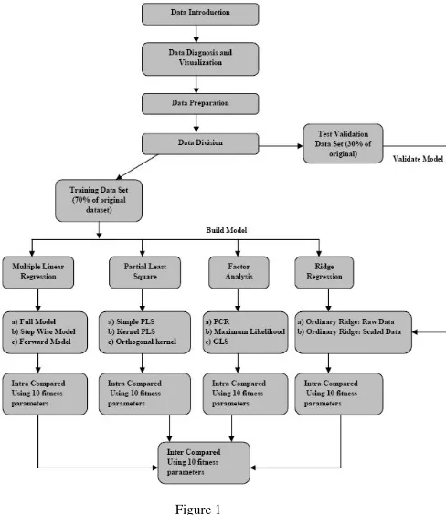
This theoretical framework should rightly called as theory for comparison of linear predictive data mining techniques. Although in this paper we focus only on four data mining techniques, yet an analyst may resort to any technique may be a linear or non linear technique. This framework will discuss the steps required for inter and intra (among the methods available within the technique) comparison. Refer to figure 1 given below.

For the purpose of evaluation of various linear predictive data mining techniques we can use three/four unique data sets. They should be unique to have a combination of the following characteristics: few predictor variables, many predictor variables, dataset with high multi-collinearity, very redundant variables and presence of outliers. A basic assumption concerned with general linear regression model is that there is no correlation (or no multi-collinearity) between the explanatory variables. When this assumption is not satisfied, the least squares estimators have large variances and become unstable and may have a wrong sign. Therefore, we resort to biased regression methods, which stabilize the parameter estimates [10].

After scaling and standardizing the data sets are divided into two parts, taking 70% observations as the “training set” and the remaining 30% observations as the “test validation set”[8]. For each data set training set is used to build the model and various methods of that technique are employed. For example in Multiple Linear Regression (MLR), three methods are associated: the full model, forward model and stepwise model. The model is validated using test validation data set and the results are presented using ten model adequacy criteria to check goodness of fit and quality of prediction. All the techniques can be intra and inter compared for their performance on the underlying unique datasets. The performance of the model can even be checked on some new dataset. This is not going to limit the study because we are not concerned with the results; we are concerned with model comparison only. Many criteria can be used to check the predictive ability of data mining technique. Almost in all such studies mentioned in the literature review section above, only two three model fitness criteria were used.

In this paper we proposed the following ten parameters like MSE, R-square, R-Square adjusted, condition number, RMSE, number of variables included in the prediction model, modified coefficient of efficiency, F-value, and test of normality.

Figure 1

The MSE of the predictions is the mean of the squares of the difference between the observed values of the dependent variables and the values of the independent variables that would be predicted by the model. It is the mean of the squared difference between the observed and the predicted values or the mean square of the residuals. MSE can reveal how good the model is in terms of its ability to predict when new sets of data are given. A high value of MSE is an indication of a bad fit. A low value is always desirable. Outliers can make this quantity larger than it actually is. MSE gives equivalent information as R-square adjusted (R2 adj.). MSE has an advantage over some process capability indexes because it directly reflects variation and deviation from the target [12].

R-square (R2 or R-Sq) measures the percentage variability in the given data matrix accounted for by the built model (values from 0 to 1).

R-square Adjusted (R2 _{adj) gives a better estimation of the} R2 because it is not particularly affected by outliers. While R-sq increases when a feature (input variable) is added, R2 adj only increases if the added feature has additional information added to the model. R2 adj values ranged from 0 to 1.

RMSE also called standard error S. It is calculated by finding the square root of MSE. The value of Sprovides an estimate of the “typical” residual, much as the value of the standard deviation in univariate analysis provides an estimate of the typical deviation. In other words, s is a measure of the typical error in estimation, the typical difference between the response value predicted and the actual response value [13]. In this way, the standard error of the estimate S represents the precision of the predictions generated by the regression equation estimated. Smaller values of s are better.

The number of variables or features included in the model: The number of variables included in a model determines how good the model will be. A good predictive DM technique accounts for most of the information available. It builds a model that gives the majority possible information representative of the system being predicted with the least possible MSE. However, when more features are added, the mean square error tends to increase. The addition of more information added increases the probability of adding irrelevant information into the system. A good data mining model selects the best features or variables that will account for the most information needed to explain or build the model.

This has been used in many fields of science for evaluating model performance [14, 15, and 16]. According to Nash et al. [15], the coefficient of efficiency can be defined as

E= 2 1 2 1

)

(

)

(

1

X

O

X

O

−

observed

of

Variance

MSE

_

_

1

₋

The ratio of the mean square error to the variance of the observed data is subtracted from unity. It ranges from -1 to +1, where -1 indicates a very bad model, since the observed mean is a better predictor than the predicted variables. A value of zero would show that observed mean is as good as the predicted model.

Te F-test is for significance of the overall regression model. One may apply a separate t-test for each predictor x1, x2, or

x3, examining whether a linear relationship exists between the target variable y and that particular predictor. On the other hand, the F-test considers the linear relationship between the target variable y and the set of predictors (e.g., {x1, x2,x3}) taken as a whole [11].

Chi-square goodness of fit test reflects how "close" are the observed values to those which would be expected under the fitted model. This test is commonly used to test association of variables in two-way tables, where the assumed model of independence is evaluated against the observed data. In general, the chi-square test statistic is of the form

X2=

−

Expected

Expected

Observed

)

(

If the computed test statistic is large, then the observed and expected values are not close and the model is a poor fit to the data. The above mentioned model fitness criteria are helpful in comparing said linear data mining techniques.

IV. THE EXPERIMENT AND RESULTS

We have used marketing dataset to experiment and validate our results. The dataset has been procured from http://www-stat.stanford.edu/~tibs/ElemStatLearn/. Dataset consists of 14 demographic variables with 8993 instances. The dataset is a good mixture of categorical and continuous variables with a lot of missing data. This is characteristic for data mining applications. In this dataset goal is to predict annual income of household from other 13 demographic variables. This dataset have been preprocessed with respect to natural log to attain log-linearity. The natural log criterion is necessary, which is the requirement of linear regression model. So, data set has been made linear.

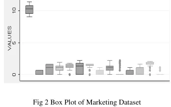
Various techniques have been applied on this underlying dataset. For models building and computing the above said ten parameters we have used various data mining tools like SPSS 17, XLstat 2009, Stata 10, Unscrambler 10.1, Statgraphics Centurion XVI and MS-Excel 2003. As all the above stated four techniques have been applied on the same dataset, leading us to decide which technique is best. Figure 2 below shows the measure of dispersion between the 14 variables of the dataset, it ranges from 0 to about 10 units. Box plot of marketing dataset shows more light on measure of dispersion between these variables, by comparing the means of all the variables.

Fig 2 Box Plot of Marketing Dataset

Refer to table 1-4, in case of factor analysis the value of R2 was found high (0.58 i.e., 58%), which is relatively more than MLR, PLS, and ridge regression techniques. It means that factor analysis has given the good fit regression line. All the models of factor analysis viz. PCR, maximum likelihood, and GLS, produced or generated high value of R2. This means on the basis of R2 factor analysis behaves best.

The adjusted R2 (adjusted for degree of freedom) was found high in case of factor analysis. It means the increasing number of independent variables in the regression model can generate again more good fit regression lines.

The ANOVA (F-value), which describes overall significance of the regression model, was found significant in all the regression models, but high in case of PLS method. It means regression extraction (influence on dependent variable) can be done significantly up-to the mark, while considering other variables. So, PLS can be regarded as best fit model to attain overall ANOVA significance.

Factor analysis was also found good for diagnosis of multi-collinearity with extraction of highest condition number. But R2 measure is considerably significant due to high value of ANOVA. It means multi-collinearity can be tolerated in factor analysis. All other techniques were found less effective to tackle multi-collinearity.

considered as good model. The MSE was found less in case of PLS techniques as compared to other techniques. So, PLS is satisfying also the BLUE criterion of regression model. PLS can be considered as good in comparison to ridge and MLR techniques.

In case of factor analysis MSE was found high, which means variance is high. So, factor analysis is not satisfying efficiently BLUE properties

.

Table I. Results of MLR model on Marketing Dataset

Table II. Results of Factor Analysis model on Marketing Dataset

Table III. Results of Ridge Regression model on Marketing Dataset

Table IV. Results of PLS Regression model on Marketing Dataset

In case of ridge regression with =0.0, which means that this value of ridge parameter can stabilize the change in standard coefficients of regression model. But as we increased the value of ridge parameter, we found considerable and desirable value of MSE for the regression modeling.

The RMSE is considered better measure than MSE. It was also found high in case of factor analysis model. So the efficiency of the regression modeling on marketing dataset is poor in case of factor analysis.

captures the influence of omitted variables from the regression model. The residual can be found through the difference between predicted and actual value of dependent variable. The

=0.25 and =0.55 model of ridge regression were found best to satisfy this.

In comparison to ridge regression model, PLS was found with good normality of residual of the regression on marketing data. The normality of residual term of the regression model is the base of BLUE properties and hypothesis testing.

So, in case of PLS and ridge techniques R2 , adjusted R2 and f-value should be considered as best estimators for regression modeling.

The normality of random term(residual term) under MLR and Factor analysis was found poor. Even factor analysis was found with highest R2 it can not be considered as good fit regression line as mentioned earlier in this paper.

The MAE was found again high in all models of factor analysis. It means we can surely state that for this dataset factor analysis is not up-to the mark to generate BLUE estimators.

Eventually we can say that a regression model will be considered as best which is satisfying usual stochastic and non-stochastic assumptions of the model since such kind of regression model (under linear regression modeling) has the capability to satisfy BLUE properties of the regression modeling.

V. CONCLUSION AND RECOMMENDATION FOR

FUTURE WORK

Based on the results obtained by comparing said linear data mining techniques, one can easily generalize and answer the following queries given in the table 5 below.

MLR and PLS techniques are simpler to understand and interpret because they do not entail high algebraic treatment. Factor analysis requires standardization to remove the effect of multicollinearity. Same is with ridge regression, which requires upto the mark scaling until model gets efficiency. Factor analysis and ridge gives good prediction as compared to PLS and MLR when the variables are truly independent. Factor analysis is best among other but some time gives results with heteroscedasticity. MLR gives poor result that may be due the effect of non-linearity in the residual term. MLR and factor analysis give stable result since R2 will be consistent with respect to scaling whereas PLS or ridge can be affected to estimators due to scaling. Ridge and factor analysis are particularly suitable when multicollinearity is there. In factor analysis up-to the mark scaling removes multicollinearity, whereas in ridge parameter scaling is required to remove multicollinearity. Factor analysis and PLS are suitable for ill conditioned data because factor analysis attempt to make component generalize which are having more effect on dependent variable, whereas in PLS only one variable is affected at a time. MLR and PLS are not good when redundant variables are there because they increase the variance, whereas ridge and factor analysis are robust against redundant variables are there residual is very small in both the techniques. Factor analysis and ridge reduces the output prediction error considerably, since R2 with low biasness is possible. MLR and PLS gives good results when all the input variables are useful due to high variance of error term. Non-linearity of the model can be easily identified through coefficient plots or plot of principle components in case of MLR, factor analysis, and ridge regression. MLR and ridge regression transforms the

data into orthogonal space as by targeting principle components and removing all discrepancies respectively.

Table V

Although, we have used the entire ten model fitness criteria’s for checking their predictive abilities. Efforts should be geared to make some criteria/s that combines the advantages of two or more of these criteria’s. Although the framework mentioned has been described for linear data mining techniques, yet the same framework can be extended to include non-linear techniques also.

VI. REFERENCES

[1] Farkas, Orsolya, and Heberger Karoly, "Comparison of Ridge Regression, PLS, Pairwise Correlation, Forward and Best Subset Selection methods for Prediction of Retention indices for Aliphatic Alcohols," Journal of

Information and Modeling, 45:2 (2005) pp. 339-346.

[2] Huang, J. et al., "A Comparison of Calibration Methods Based on Calibration Data size and Robustness," Journal

of Chemometrics and Intelligent Lab. Systems, 62:1

(2002) pp. 25-35.

[3] Vigneau, E., M. F. Devaux, and P. Robert, "Principal Component Regression, Ridge Regression, Ridge Principal Component Regression in Spectroscopy Calibration," Journal of Chemometrics, 11:3 (1996) pp. 239-249.

[4] Malthouse, Edward C., "Ridge Regression and Direct Marketing Scoring Models," Journal of Interactive

Marketing, 13:1854 (2000), pp.16-23.

[5] Naes, T., C. Irgens, and H. Martens, "Comparison of Linear Statistical Methods for Calibration of NIR Instruments," Applied Statistics, 35:2 (1986), pp.195-206. [6] Hassan Al.M.Yazid, and Kassab Al.M.Mowafaq, “A

[7] Noori R., Abdoli M.A, Ghazizade, and Samieifard R, “Comparison of Neural Network and Principal Component Regression Analysis to Predict The Solid Waste Generation in Tehran”, Iranian J Publ Health, vol. 38, no.1, 2009, pp.74-84.

[8] Yeniay O, and Goktas A., “ A Comparison of Partial Least Square Regression with Other Prediction Methods”, Hacettepe Journal of Mathematics and Statistics, vol.31,2002, pp.99-111

[9] Lonial Z, and Subhash L, “ Comparison of performance of several data mining methods for bad debt recovery in healthcare industry”, The journal of applied Business Research, volume 22, no. 2, 2005

[10]Al-Kassab M, “A Monte Carlo Comparison between Ridge and Principal Components Regression Methods” Applied Mathematical Sciences, Vol. 3, 2009, no. 42, 2085 - 2098

[11] Myatt J. Glenn, “Making Sense of Data-A practical guide

to exploratory data analysis and data mining” New Jersy:

Wiley-Interscience (2007).

[12] Battaglia, Glenn J., and James M. Maynard, "Mean Square Error: A Useful Tool for Statistical Process Management," AMP Journal of Technology 2 (1996), pp. 47-55.

[13] Larose T. Daniel, “Data Mining-Methods and Models” Wiley Interscience, (2002).

[14] Legates, David R. and Gregory J. McCabe, "Evaluating the Use of Goodness of Fit Measures in Hydrologic and Hydroclimatic Model Validation." Water Resources

Research, 35:233-241 (1999).

[15] Nash, J.E. and J.V. Sutcliffe, "Riverflow Forecasting through Conceptual Models: Part 1-A Discussion of Principles." J. Hydrology, 10 (1970), pp. 282-290. [16] Willmott, C.J., S.G. Ackleson, R.E. Davis, J.J. Feddema,

K.M. Klink, D.R.Legates, J. O'Donnell, and C.M. Rowe, "Statistics for the evaluation and comparison of models."